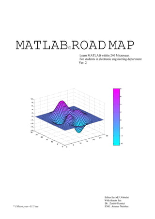
MATLAB©ROAD MAPLearn MATLAB within 240 Microyear.
For students in electronic engineering department
Ver: 2
Edited by:M.F.Nabulsi
With thanks for:
Dr. Zoubir Hamici
* 1Micro year=31.5 sec ENG. Ammar Natshee
INTRODACTION:
MATLAB (MATRIX LABORATORY) is a
scientific programming language directed for
engineer who don't know how to program,
In general the most of IT students do not know how
to program by Matlab.
Because they don't know some things like
frequency domain or other engineering
parameters….
So you can be one of the experts who know how to
deal with MATLAB.
So go ahead and learn MATLAB.
***************************
Index:
CH1 starting MATLAB 1
CH2 Matrices 1
2.1 inserting a matrix:
2.2 merging matrices:
2.3 Selecting a peace of a Matrix:
2.3.1selecting a certain element of matrix
2.4 creating a unit Matrix:
2.4.1 Creating zeros matrix
2.4.2 Creating ones matrix
2.4.3 Creating any matrix
2.4.4 Creating eye matrix
2.5 deleting a certain column or row
2.6 saving matrix
2.7 loading matrix
2.8 Matrices operation:
2.8.1 Adding (+):
2.8.2 Subtracting ( - ) :
2.8.3 Multiplying ( * ):
2.8.4 dividing (/):
2.8.5 Summing
2.8.6 Rising to power:
2.8.7 Matrix transpose
2.8.8 Diagonal of matrix
2.8.9 Upper triangular
2.8.10 lowers triangular
2.8.11 Matrix flipping:
2.8.12 reshaping matrix
2.8.13 reordering matrix
2.9 size and length of Matrix:
2.10 logical operations on matrix
2.10.1 Comparator
2.10.2 comparing two matrices
2.10.3 (and, or) operation
2.10.4 Absolute value
2.11 The 'find' function
2.12 For ,while ,if instructions:
2.12.1 for loop
2.12.2 While loop
2.12.3 (if, else if , else) inst
CH3 arithmetic operation:
3.1 Complex number
3.2 Approaching: (round fix floor ceil )
3.3 basic functions:
3.3.1 Square root:
3.3.2 Reminder
3.3.3 Exponential
3.3.4 signum function
3.3.5 Trigrometric function:
3.4 polynomial:
3.5 polynomial operations (* / + -) :
3.5.1 Multiplying two polynomials
3.5.2 dividing two polynomials:
3.5.3 Adding subtracting two
polynomials:
3.5.4 dividing with reminder:
3.6 Derivative
3.7 integration:
3.7.1 integrating basic function:
3.7.2 integrating undefined function:
3.7.3 double integration
CH4 Plotting:
4.1 (2D) graphic:
4.1.1 data plotting
4.1.2 polynomial equation plotting
4.1.3 basic function plotting(sin cos tan
exp…)
4.1.4 stem plot:
4.1.5 polar plot
4.1.6 complex plot:
4.2 (3D) graphic
CH5 control system:
5.1 zeros&poles:
5.2 bode plot:
5.3 nyquest plot:
5.4 step response plot:
5.5 root locus plot:
CH6 DSP:
6.1 sampling (sin) signal
6.2 Loading a wave file
6.3 Loading an image file
6.4 encryption & decryption
6.4.1 Encrypting an image:
6.4.2 Decrypting an image:
6.4.3 Encrypting an audio file:
6.4.4 Decrypting an audio
6.5 RADAR SYSTEM:
6.6 fast Fourier transform function (FFT)
6.7
*******************************
***********************
*************
********
1
CH 1:
Statrting MATLAB:
You have two choices to
start MATLAB:
1) Open MATLAB
main window and directly
write your command like:
>>5*5+2.5
ans=
12.5
This method is useful to
write a quick commands or
even a small programs but
not useful at all in long
programs.
2) Open an m-file then write
your program.
Save it.
Then run it………
Note:
MATLAB understands
nothing except Matrix even
when you write
>>M=5+4
MATLAB will define 5 as a
1*1 matrix and 4 also as 1*1
matrix,
Then MATLAB will add the
two matrices to get a new
1*1 matrix (M).
Even when you load an
audio file into MATLAB
, MATLAB will define it as
2D matrix.
Also MATLAB will define
an image as 3D matrix, you
will see that latter
%useful note:
- writing the (%) (prsentage
sgin) in matlab enables you
to write your comment after
the sign.
-TRY TO PRESS
CNTRL+k in matlab this
command will enable you to
delete the line until the end
%try to type …. (Dots)
This enable you to move to
next line without executing
the command
Ex:
A=[1 2 3 4 5 7 8 9 5 6 4….
4 5 6 55 0];
**********
CH 2:
Matrices:
2.1 inserting a matrix:
%to load your matrix use [ ]
%to move to next element
use space
%to move to next row use
(;)
EX:
>> a=[1 2 3;4 5 6;7
8 9]
a =
1 2 3
4 5 6
7 8 9
2.2 merging matrices:
EX:
Consider the following two
matrices a and b
>>a=[2 4 1]
a =
2 4 1
>> b=[0 7 9]
b =
0 7 9
1)write a matlab command to
put the 2 matrices a & b
above each other
hint: use [ ] and ;
Sol:
>> c = [a;b]
c =
2 4 1
0 7 9
2)write a command to put
the 2 matrices a & b behind
each others (on the same
raw)
hint: use [ ] and spaces.
Sol:
>> c=[a b]
c =
2 4 1 0 7 9
2.3 Selecting a peace of
Matrix:
EX:
Select the 2nd
and the 3rd
row of the given matrix (a)
%Hint:
to select a certain rows or
column of the whole matrix
use ( ) and ,
>>a= [1 2 3 4; 5 6
7 8; 9 10 11 12]
Ans:
a =
1 2 3 4
5 6 7 8
9 10 11 12
2
>> b=a(2:3,:)
Ans:
b =
5 6 7 8
9 10 11 12
%2:3 means select rows
from 2 up to 3
%: Means select all columns
EX:
Select only the 3ed column
of matrix a
Sol:
>> x=a(:,3)
x =3
7
11
EX☺
Select the 1st
column of
matrix (a) and the 2nd
column of matrix (a) and put
them above each other
Sol:
>>
z=[a(:,1);a(:,3)]
z =
1
5
9
3
7
11
%try this
>> s=a(2:3,2:3)
Ans:
s =
6 7
10 11
2:3 means select rows 2 & 3
2:3 means select column2&3
2.3.1 selecting a certain
element of a MATRIX:
EX:
let
>>x=[5 27 5 13 8 1]
x =
5 27 5
13 8 1
select the 2nd
element of the
matrix x:
SOL:
>> y=x(2)
y =
27
select the 2nd
element up to
the 5th
element :
SOL:
>> y=x(2:5)
y =
27 5 13
% select the 3ed element up
to the end of the matrix X
SOL:
>> y=x(3:end)
y =
5 13 8 1
%select the 3ed element
down to the 1st
element
SOL:
>> y=x(3:-1:1)
y =
5 27 5
%-1 means move back by
one element.
%select the 1st
, 2nd
and
6th
element of matrix x
SOL:
>> y=x([1 2 6])
y =
5 27 1
2.4 creating a unit
Matrix:
2.4.1 creating zeros matrix:
>> x=zeros(2,5)
x =
0 0 0 0 0
0 0 0 0 0
2.4.2 creating ones matrix:
EX:
Create a ones matrix consists
of 3 col and 3 row
SOL
>> x=ones(3)
Or x = ones(3,3)
Ans:
x =
1 1 1
1 1 1
1 1 1
EX:
Create 3by1 ones matrix
>> x=ones(3,1)
sol:
x =
1
1
1
2.4.3 creating any matrix:
EX:
Create a 2by2 (fives) matrix
Sol:
>> x=5*ones(2)
Or x=5*ones(2,2)
Ans:
x =
5 5
5 5
2.4.4 creating eye matrix:
>> x=eye(3)
x =
1 0 0
0 1 0
0 0 1
3
>> x=eye(2,3)
x =
1 0 0
0 1 0
>> x=eye(3,2)
x =
1 0
0 1
0 0
2.5 deleting a certain
column or row of
matrix:
EX:
Delete the 2nd
and the 4th
column of matrix N.
Where
N =
1 4 7 10
2 5 8 11
3 6 9 12
Sol:
>> N ( : , [2 3] ) = [ ]
: all rows
[2 3]col2& col3
ans:
N =
1 10
2 11
3 12
2.6 saving a matrix:
EX:
Given:
a=
1 2
3 4
b=
4 7
5 9
c=a+b;
save matrix A and
matrix c
sol:
>>save anyname.mat a c
2.7 loading a matrix:
>>load name.mat
%this instruction
will load matrices
a and c to MATLAB
workspace*.
*workspace=memory
2.8 Matrices operation:
given two matrices:
>> a=[1 2;3 4]
a =
1 2
3 4
>> b=[5 6;7 8]
b =
5 6
7 8
2.8.1 Adding (+):
EX:
add matrix a to matrix b
sol:
>> a+b
ans =
6 8
10 12
2.8.2 subtracting ( - ) :
EX1:
Subtract matrix a from b
Sol:
>> a-b
ans =
-4 -4
-4 -4
EX2:
Given matrix ( y)
>> y=1:9
y =
1 2 3 4 5 6 7 8 9
subtract 9 from each element
of matrix y.
sol:
>> y=9-y
ans:
y =
8 7 6 5 4 3 2 1 0
2.8.3 multiplying ( * ):
EX1:
Multiply matrix a
by matrix b.
Sol:
>> a.*b
ans =
5 12
21 32
Note:
If you put a dot
after matrix (a)
matlab will do an
element by element
multiplication
not(matrix by
matrix
multiplication.
EX2:
Multiply 2 by matrix a then
subtract b
Sol:
>> 2*a-b
ans =
-3 -2
-1 0
2.8.4 dividing (/):
EX1:
Divide matrix a over b
(Element by element
division.)
Sol:
>> a./b
ans =
0.2000 0.3333
0.4286 0.5000
EX2:
%2/a
>> 2./a
4
ans =
2.0000 1.0000
0.6667 0.5000
2.8.5 Summing
EX1:
GIVEN matrix c
>> c=[4 5 3;2 4 1;0
2 5]
c =
4 5 3
2 5 1
0 2 5
find the sum of each column
SOL:
>> sum(c)
ans =
6 12 9
Where:
4+2+0=6
5+5+2=12
3+1+5=9
EX2:
Find the sum of each row.
SOL:
>> sum(c')
ans =
12 8 7
Where:
4+5+3=12
2+5+1=8
0+2+5=7
2.8.6 average:
EX:
Find the average of matrix a
>>a=[5 6 8 7 4 3 2
1 4 -5]
Sol:
>>L=length(a)
>>avg=sum(a)/L
avg =
3.5000
2.8.7 rising to power:
EX1:
Givin matrix a
A=
1 4
9 16
Find a^2
sol:
>> a.^2
ans =
1 4
9 16
EX2:
%1/a
>> a.^-1
ans =
1.0000 0.5000
0.3333 0.2500
2.8.8 Matrix transpose
EX:
Give matrix a
a=
1 2 3
4 5 6
7 8 9
find the transpose* of matrix
a
SOL:
>> a'
ans =
1 4 7
2 5 8
3 6 9
Transpose*: each row will be
column and each column will be
row
2..8.9 diagonal of matrix
given matrix x
>> x=[1 2 3;4 5 6;7
8 9]
x =
1 2 3
4 5 6
7 8 9
find the diagonal of the
matrix (x). and save it into
matrix b.
Sol:
>> d=diag(x)
d = 1
5
9
2.8.10 upper triangular
EX:
given matrix x
x =
1 2 3
4 5 6
7 8 9
Find the upper
triangular of
matrix x and save
the answer in
matrix u
SOL:
>> u=triu(x)
u =
1 2 3
0 5 6
0 0 9
2.8.11 lower triangular:
Find the lower
triangular of
matrix x and save
the answer in
matrix L
SOL:
>> L=tril(x)
L =
1 0 0
4 5 0
7 8 9
2.8.12matrix flipping:
EX1:
Given matrix b
b =
1 2 3
4 5 6
7 8 9
Flip matrix b (up-down)
5
SOL:
>> f=flipud(b)
ans:
f =
7 8 9
4 5 6
1 2 3
EX2:
flip matrix b (left-right)
(mirror effect).
SOL:
>> LR=fliplr(b)
LR =
3 2 1
6 5 4
9 8 7
2.8.13 reshaping matrix
EX:
Given matrix a
>> a=1:12
a =
1 2 3 4 5 6 7 8 9 10 11 12
reshape matrix (a) into
(2by6) matrix
SOL:
>> r=reshape(a,2,6)
answer
r =
1 3 5 7 9 11
2 4 6 8 10 12
EX2:
Reshape matrix a to (4by3)
matrix
SOL:
>> r=reshape(a,4,3)
r = 1 5 9
2 6 10
3 7 11
4 8 12
%try this (reshape with
transpose): note the
difference
r=reshape(a,4,3)'
r =
1 2 3 4
5 6 7 8
9 10 11 12
2.9.14 reordering matrix:
%this command will enable
you to re organize your
matrix in the way you
like(by interchanging the
position of any columns or
rows)
EX:
Given a
>>a =
1 4 7 10
2 5 8 11
3 6 9 12
Interchange between col 2
and col3
SOL:
>> b=a(:,[1 3 2 4])
b =
1 7 4 10
2 8 5 11
3 9 6 12
2.9 size and length of
Matrix:
EX:
%find the size of matrix a
>> a = [1 2 3 4
; 5 6 7 8]
a =
1 2 3 4
5 6 7 8
SOL:
>> s = size(a)
answer:
s =
2 4
%witch mean that
matrix a is a 2by4
matrix.
EX2:
%find the length of matrix b
b =
1 2 3 4 5 6 7 8
SOL:
>> L=length(b)
L =
8
2.10 logical operation
on matrix
2.10.1 comparator:
EX:
Given matrix a
a=
0.2 -0.8 0.7 1.2 0 0 2
6
Estimate the position of each
element greater than 0.5
SOL:
>> y=a>0.5
y =
0 0 1 1 0 0 1
%this will give only a logic
value of each element in
matrix (a) which is greater
than 0.5
2.10.2 comparing two
matrices
EX:
Given a & b
a=
0.2 -0.8 0.7 1.2 0 0 2
b =
100 -.8 0.7 1.2 99 99 2
compare between mat a &
mat b
SOL:
>> c= a= =b
c =
0 1 1 1 0 0 1
% 0's and 1's are a logic
value where the value 1
indicate to the position
where element a equal
element b.
2.10.3 (and, or) operation:
EX:
Given a
a =
1 2 3 4 5 6 7 8 9
find the position of each
element witch is
greater than 2
&
smaller than 6
>> c= (a>2) & (a<6)
c =
0 0 1 1 1 0 0 0 0
2.10.44absolut value:
EX:
given matrix x
>> x=-3:3
x =
-3 -2 -1 0 1 2 3
1)find the position of each
element which is greater
than 1 (in absolute value).
2)create a new matrix which
contains only the element
which is greater than 1 (in
absolute value)
SOL:
1) z=abs(x)>1
z =
1 1 0 0 0 1 1
%LOGIC VALUE
2) z=x(abs(x)>1)
z =
-3 -2 2 3
%REAL VALUE
2.11 the 'find' function:
EX:
Find the position of each
element in matrix (a) which
is greater than one (in
absolute value)
Where:
a= -2 -1 0 1 2 3 4
SOL:
>> find(abs(x)>1)
ans =
1 5 6 7
%1 2 6 7 mean that
the 1st 2nd
6th
and 7th
Positions of matrix a is
greater than 1 (in absolute
value)
EX2:
Given marix a
a =
4 5 6 7 8 9 8 7 6 5 4
find the position of each
element witch is greater than
7.
SOL:
>> f=find(a>7)
f =
5 6 7
7
%the 5th
, 6th
and 7th
position is greater than 7
2.12 for, while ,if
instructions :
2..12.1 for loop:1.1
EX!:
For a Given matrix n.
Create a new matrix (x)
which contains the square of
each element in matrix n (by
using for inst)
SOL:
>> for n=1:10
x(n)=n^2;
end
x =
1 4 9 16 25 36 49
64 81 100
EX (double for loops):
>> for m=1:4
for n=1:4
s(m,n)=m+n
end
End
Answer:
s =
2 3 4 5
3 4 5 6
4 5 6 7
5 6 7 8
2..12.2 while loop:
EX simple while loop:
B=1
While b<5
b=b+1
end
2..12.3 (if else if else) inst:
EX(simple):
if ((attendance >=
30)&(grade >= 25))
total = 100.;
elseif ((attendance
>= 20)&(grade_a>=
12))
total = 50;
else
total=0
end;
CH3:
Arithmetic operation:
3.1 Complex number
>> m=1-2*i
m = 1.0000 -
2.0000i
>> m=abs(1-2*i)
ans:
m =2.2361
>> a=angle(1-2*i)
ans:
a =-1.1071
%a is radian to convert to
degree =>
>> Degree=a*180/pi
Degree =63.4349
>> r=real(1-2*i)
r =1
>> x=conj(1+i)
x =1.0000 - 1.0000i
3.2 Approaching:
%Approach to nearest
integer
------> integer
>> a=round(2.2)
a =2
%Approach to zero
------> 0
>> a=fix(2.8)
a =2
%Approach to –inf
------> - ∞
>> a=floor(2.8)
a =2
%Approach to +inf
------> ∞
>> a=ceil(2.8)
a =3
3.3 basic functions:
3.3.1 square root:
>> x=sqrt(16)
x =
4
3.3.2 reminder
>> r=rem(9,2)
r =
1
%9/2=4 and the reminder is
1
3.3.3 exponential
>> e=exp(1)
e =
8
2.7183
3.3.4 signum function
>> a=sign(2)
a =
1
>> a=sign(-3)
a =
-1
>> a=sign(113)
a =
1
>> a =sign(-113)
A=-1
3.3.5 trigrometric function:
>> a=sin(pi/2)
a =
1
>> a=cos(pi)
a =
-1
>> a=tan(pi/4)
a =
1.0000
>> a=asin(0.5) %sin inverse
a =
0.5236 % in radian
>> a*180/pi
ans =
30.0000 %in degree
>> %also see {acos atan sinh
cosh tanh asinh acosh}
3.4 polynomial:
let
y(x)=x^2 + 4x + 4
• to insert this equation
into Matlab
type the following:
>> y=[1 4 4]
y =
1 4 4
• to find the roots of
this equation
type the following
>> r=roots(y)
ans:
r =
-2
-2
now you can write
y=(x+2)(x+2)
• if you already have
the roots and you
need to find the
equation
type the following
>>r=
>> y=poly(r)
ans:
y =
1 4 4
EX:
Consider the equation below:
Y(x)= (x-1) (x-4) (x-9) (x+3)
Open the bracket of this
equation.
i.e.: find the original 4th
order equation.
Hint: 1 4 9 -3 represent the
roots of this equation
Sol:
>> r=[1 4 9 -3]
>> y=poly(r)
y =
1 -11 7 111 -108
%now we can write:
y= x^4 - 11 x^3 +7x^2
+111x -108
3.5 polynomial
operation (* / + -) :
3.5.1 Multiplying two
polynomials:
EX:
For the given two equations:
y1= x^2 + 4x + 4
y2= 2x^2 + 5x + 5
Find z= y1 * y2
SOL:
>> y1=[1 4 4];
>> y2=[2 5 5];
>> z=conv(y1,y2)
z =
2 13 33 40 20
%which means:
z=2 x^4 +12x^3 +33x^2
+40x +20
9
3.5.2 dividing two
polynomials:
EX:
Find the division of equation
z over equation y2.
SOL:
>> d=deconv(z,y2)
d =
1 4 4
3.5.3 Adding subtracting
two polynomials:]
EX:
find y1+y2
SOL:
>> c=y1+y2
ans:
c =
3 9 9
% i.e: c=3x^2 + 9x + 9
EX:
find w=z-y1
SOL:
>> w=z-y1
Answer:
[??? Error using
==> -
Matrix dimensions
must agree.]
%to solve this problem we
should write:
>> w=z-[0 0 y1]
answer:
w =
2 13 32 36 16
%note: when u add or
subtract two polynomial they
should have the same order.
3.5.4 dividing with
reminder:
In general if you divide two
equations
y1= 4x^3 + x^2 + 4x + 4
y2= x^2 + 4x + 4
you get a result and reminder
EX:
>> y1=[4 1 4 4]
y1 =
4 1 4 4
>> y2=[1 4 4]
y2 =
1 4 4
[q,r]=deconv(y1,y2)
ans:
q = 4 -15
r = 0 0 48 64
%q represents
division result
%r represent
division reminder
3.6 Derivative
EX:
Drive the following equation
y= x^4 - 11 x^3 +7x^2
+111x -108
i.e.: (find dy/dx)
SOL:
>> y=[1 -11 7
111 -108]
>> driv=polyder(y)
answer:
driv =
4 -33 14 111
%=>
dy/dx= 4x^4
-33x^3 + 14x^2 + 111
3.7 integration:
3.7.1 integrating basic
functions:(sin, cos, exp...)
EX1:
Integrate a sin function from
0 to pi4
SOL:
>>quad('sin',0,pi/4)
ans =
0.2929
EX2:
Integrate an exp function
from 0.8 to 1.6
SOL:
>> quad('exp', 0.8 , 1.6 )
ans =
2.7275
10
3.7.2 integrating undefined
function:
EX:
Integrate the function
y=x^2 + x
From x=2
To x=5.6
Sol:
% to achieve this integration
you should define this
function (y=x^2 +2x)
1) Open a new m-file
type the following:
>>function
z=myfunction1(x)
>>z=x.^2 + 2*x
%don't forget the dot
2) save this m-file with the
name (myfunction.m)
or you can select any other
name else it's up to u.
3) NOW go to matlab main
window and type the
following:
>>quad('myfunction',2,5.6)
ans =
58.2773
3.7.3 Double integration:
EX:
Integrate the following
equation twice
Z=sin(x)cos(y)+1
over a period
x 1 pi
y 0 2pi
sol:
Open new m-file
>>function z=myfun(x,y)
>>z=sin(x)cos(y)+1
%save it.
%NOW go to matlab main
window and type:
>>dblquad('myfun',1
,pi,0,2*pi)
ans=
13.4560
*********************
*************
CH4:
Plotting:
4.1 (2D) graphic:
4.1.1 DATA PLOTING
>> x=[0 2 1 3 4 3 5 4 6 5 7 6
9];
>> Plot(x)
%THIS IS A SIMPLE DATA
PLOTING THE (X) AXIS
REPRESENT THE DATA
POSITION AND THR (Y)
AXIS REPRESENT THE
VALUE OF THIS POSITION
0 2 4 6 8 10 12 14
0
1
2
3
4
5
6
7
8
9
4.1.2 polynomial equation
plotting:
EX:
Plot the function y=x^2
SOL:
>> y=[1 0 0];
>> x=-100:0.1:100;
%0.1 to set the
accuracy of your
graph
>> v=polyval(p,x);
>> plot(x,v);
>> xlabel('x');
>> ylabel('y');
>> title('y=x^2')
4.1.3 basic function
plotting (sin cos tan
exp......):
EX 1:
Plot a sin and cos function
on the same graph over a
time period t=1 10
SOL:
11
>> t= 0 : 0.1 : 10;
>> y=sin(t);
>> z=cos(t);
>> plot ( t , y , 'b+' , t , z ,
'R*')
>> xlabel('time');
>> ylabel('volt');
>> grid
>> text(3,0.45,'sin t')
>> text(.8,0.3,'cos t')
%note 1:
when you type
>> plot ( t , y , 'b+' )
b means graph color is blue.
+ means: plot the graph by
using the (+) sign.
% Color options:
b blue c cyan
g green y yellow
r red k black
% signs options:
. point . dash dot
- solid x x-mark
o circle + plus
: dotted -- dashed
* star s square
%note 2:
to plot a certain region of
your graph (to focus on a
certain region)
type this
>> axis([5 10 0
1])
%where Xmin= 5
Xmax= 10
Ymin= 0
Ymax= 1
EX 2:
Draw three phase voltage on
the same graph.
Where
f=50hz.
draw 2 cycles.
Vmax=5 volt.
Sol:
Method 1:
>>t= 0 : .3e-3 :
2*20e-3 ;
%T= 20ms =20e-3= 1/50hz
%2*20e-3 because we need
to draw two cycles .
%(0.3e-3) sets the accuracy
of your graph, the smaller
number the higher accuracy
>>v1=5*sin(2*pi*50*t);
% pahse1 is v1=5sin(2∏ f t)
>>v2=5*sin(2*pi*50*t-
2*pi/3);
>>v3=5*sin(2*pi*50*t+2*pi
/3);
>>plot
(t,v1,'b*',t,v2,'g+',t,v3,'r:')
>>xlabel('time');
>>ylabel('volt');
method2 (hold on):
Plot (t,v1,'b*')
Hold on
Plot (t,v2,'g+')
Plot (t,v3,'r:')
Hold off
%hold on: enable you to plot
on the same graph sheet
%you will get the same
graph shown above
method 3 (subplot):
subplot(2,2,1)
plot (t,v1,'b*')
subplot(2,2,2)
plot (t,v2,'g+')
12
subplot(2,2,3)
plot (t,v3,'r:')
%what dose 'subplot(2,2,3)'
Means:
%2,2 means: create a
graphic Which contains two
rows and two columns of
small graphic sheets
% ,3 means: draw in the 3ed
graphic sheet
%try this
% draw this
y= sin(x)/cos(x)
>>x=0:0.05:2*pi;
>>w=sin(x)./cos(x)
>>plot(x,w)
%Note: don't forget to put
a DOT after sin(x), or you
will get matrix mismatching
error.
4.1.4 Stem plot:
EX:
Plot a sin wav as stem plot.
SOL:
>>t = 0:0.2:2*pi;
>>x = sin(t);
>>stem(t,x)
0 1 2 3 4 5 6 7
-1
-0.8
-0.6
-0.4
-0.2
0
0.2
0.4
0.6
0.8
1
EX ☺ (try this):
>>x = 0 : 1 : 40 ;
>>y = sin(x).*exp(-0.05*x);
%this represent the equation
of decaying sin.
>>plot(x,y,'--rs',...
>>'LineWidth',1,.....
>>'MarkerEdgeColor','k',...
>>'MarkerFaceColor','g',...
>>'MarkerSize',8)
Notes:
%rs: means color is red with
equare mark.
%the dots at the end of each
lines means that you can
move safely to the next line
(because this command is
too long)
% note: (important):
>>x=-2*pi : pi/10 :
2*pi;
>>y=sin(x);
>>z=20*cos(x);
>>subplot(2,1,1)
>>plot(x,y,x,z)
>>subplot(2,1,2)
>>plotyy(x,y,x,z)
%plotyy is an important
command it gives all
functions the same scale.
plot:
plotyy:
4.1.5 polar plot
>>theta=0:0.05:2*pi
;
>>x=sin(3*theta)
>>polar(theta,x)
4.1.6 complex plot:
>>z=[0 1+i 2+i 2+2i 3+3i]
>>plot(z)
%matlab will draw 4 points
on the complex plan; also
matlab will connects these
points
13
4.2 (3D) graphic:
EX 1:
Plot a Helox
t= 0: 0.05 : 10*pi;
y=sin(t);
z=cos(t);
plot3(y,z,t)
grid
EX 2 (hard):
>>x=0:0.1:3*pi;
>>z1=sin(x);
>>z2=1.5*sin(2*x);
>>z3=2*sin(3*x);
>>y1=zeros(size(x));
>>y2=ones(size(x));
>>y3=2*ones(size(x));
>>plot3(x,y1,z1,x,y2,z2,x,y3
,z3)
%in this ex we've plotted
three SIN signal (z1 ,z2 , z3)
in 3D plane .
%the 1st
sin signal z1 plotted
in plane y1=0
%the 2nd sin signal z2
plotted in plane y2=1
%the 3ed sin signal z3
plotted in plane y3=2
***********************
CH5:
control system:
5.1 zeros&poles:
EX:
Consider the flowing
controlled system.
Find zeros and poles.
%numerator = 10
%denominator= s^2 + 4s + 3
in Matlab
>> num=10;
>> den=[1 4 3];
>> [z,p,m]=tf2zp(num,den)
z =
Empty matrix
p = -3
-1
m =
10 %gain
EX:
For the given zeros and poles
shown above, find the
transfer function
Sol:
>> z=[];
>> p=[-3 -1];
>> m=10;
>>
[num,den]=zp2tf(z,p,m)
num =
0 0 10
den =
1 4 3
5.2 bode plot:
T.F= 10
S^2 + S + 3
>> num=10;
>> den=[1 1 3];
>> bode(num,den)
-60
-50
-40
-30
-20
-10
0
10
20
Magnitude(dB)
10
-1
10
0
10
1
10
2
-180
-135
-90
-45
0
Phase(deg)
Bode Diagram
Frequency (rad/sec)
5.3 nyquest plot:
>> nyquist(num,den)
>> grid
T.F= 10
S^2+4s+3
U(s) Y(s)
-3 -2 -1 0 1 2 3 4 5
-6
-4
-2
0
2
4
6
0 dB
-10 dB
-6 dB
-4 dB
-2 dB
10 dB
6 dB
4 dB
2 dB
Nyquist Diagram
Real Axis
ImaginaryAxis
14
5.4 step response plot:
>> step(num,den)
>> grid
0 2 4 6 8 10 12
0
0.5
1
1.5
2
2.5
3
3.5
4
4.5
5
Step Response
Time (sec)
Amplitude
5.5 root locus plot:
EX:
Find the root locus for the
given system.
sol:
>> num=[1 6];
>> x1=[1 4 0];
>> x2=[1 4 8];
>> den=conv(x1,x2);
>> rlocus(num,den)
>> grid
-12 -10 -8 -6 -4 -2 0 2 4 6
-10
-8
-6
-4
-2
0
2
4
6
8
10
0.72 0.6 0.46 0.3 0.16
0.3 0.16
0.98
0.92
0.84
0.84
0.6 0.46
8
0.72
0.92
10 6
0.98
24
Root Locus
Real Axis
ImaginaryAxis
***********************
***************
CH 6:
DSP :
6.1 sampling a (sin)
signal:
EX:
For the sinusoidal function
below:
X(t) = 3 sin(2.∏.fm.t)
Find the number of samples
from 0 up to 2sec
Where fs=100hz
fm=10hz
Sol :
>> fm=10;
>> fs=100;
>> t=0:1/fs:2;
>>
x=3*sin(2*pi*fm*t);
>> L=length(x)
>> figure(1)
>> plot(x)
>> figure(2)
>> plot(t,x)
L =
201
figure 1
figure 2
0 0.2 0.4 0.6 0.8 1 1.2 1.4 1.6 1.8 2
-3
-2
-1
0
1
2
3
% note that figure 1 has the
same shape of figure 2.
But:
%Figure 1 (plot(x)): the
vertical axis is the amplitude
axis & the horizontal axis is
the element position axis:
%Figure 2 ( plot ( t, x ) ): the
Vertical axis is also the
amplitude axis but the
horizontal axis is the TIME
axis.
%L=201 represent the
number of sample
within t=2sec period.
Indeed we have 200 sample
but the matlab start counting
the sample from time t=0sec
%to avoid this write
>> t = 1/fs : 1/fs : 2 ;
L=
200
T.F= k (s+6)
s(s+4)( s^2+4s+8)
U(s) Y(s)
% so matlab will start
counting from the first
sample.
15
6.2 Loading an audio
wave file:
EX:
>>
[data,fs,bitpersample]
=
wavread('c:click.wav')
;
S=size(data)
L=length(data);
t = 0 : 1/fs : (L-1)/fs
;
>> plot(t,data)
ans:
L =
7168
S=
7168 2
%from the size of data, we
conclude that Matlab stores
the wave file as a
2dimitional matrix of two
column (if stereo) and 7168
rows which is the number of
samples in the wave file
0 0.05 0.1 0.15 0.2 0.25 0.3 0.35
-1
-0.8
-0.6
-0.4
-0.2
0
0.2
0.4
0.6
0.8
1
6.3 Loading an image
file:
>> img = imread
('c:tree.bmp','bmp
');
>> size(img)
ans =
126 188 3
%note that in general
whenever you type (size)
you get 2 numbers the 1st
represents the number the of
rows of your matrix and the
2nd
represents the number of
columns.
But in this example when we
typed
Size(img) we have got 3
numbers.
Indeed matlab stores colored
images as 3dimintional
matrix.
So
Size= 126 188 3
126: represent the number
of rows or(width of the
image)
188: represent the number
of column or (length of
image)
3: matlab will save each base
color(RGB) in separate
dimension so the first
dimension contains red color
only ,
And the 2nd
contains green
color,
And the 3ed dimension
contains blue
(RGB)
6.4 encryption&
Decryption:
6.4.1 Encrypting an image:
EX:
Write a matlab program to
encrypt a Bmp image witch
saved in path c:image.bmp
SOL:
%to write an encryption
program you have to follow
5 steps:
%step 1:
%loading the image into
matlab
>>img = imread
('C:image.bmp','bmp');
%step 2:
%generating the key matrix
[password]:
>>s=size(img);
>>width=s(1);
>>for i=1:width;
en(i)=i;
end;
%note: size of the
key is the same as
the width of the
image.
16
%randomizing the
key
>>for i=1:2*width
ix = round
((width1)*rand(1)+1
);
jx = round
((width-
1)*rand(1)+1);
bk=en(ix);
en(ix)=en(jx);
en(jx)=bk;
end;
%step 3:
%saving the key
matrix.
>>save key.mat
%Step 4:
%encrypting the
image.
>>encimg=img;
for j=1:width;
encimg(en(j),:)=img
(j,:);
end;
%step 5:
%saving the
encrypted image.
>>imwrite(img2,'c:
encrypted
image.bmp’,’bmp’)
Encrypted image.bmp
6.4.2 decrypting an image:
EX:
Write a MATLAB program
to
Decrypt the previous image
SOL:
%decryption is done
by 4 steps
%step 1:
%reading the
encrypted file
encimg=imread('c:t
est1.bmp','bmp');
%step 2:
%loading the key
load key.mat;
%step 3:
%decrypting th
image
s=size(encimg);
width=size(2);
decimg=encimg;
for j=1:width;
decimg(j,:)=encimg(
en(j),:);
end;
%step 4:
%saving the
deyrepted image:
imwrite(img3,'c:de
crepted
image.bmp’,’bmp’)
Decrypted image.bmp
6.4.3 Encrypting an audio
file:
EX:
Write a matlab program to
encrypt an audio file, the
program should divide the
audio file into segments,
where each segment consists
of 128 elements,
and then encrypt each
segment by one key.
SOL:
%note: this policy of
encryption is used by (wi-
fi)(802.11) wireless digital
communication.
%step 1:
%loading the audio
file
[x,fs,bps]=wavread(
'c:audio.wav');
%step 2:
%defining the
needed variables
l=length(x);
BM=ceil(l/1024);
%bm represent the
number of blocks in
the file where each
block contains
1024 element
zero=zeros(BM*1024-
l,1);
17
xz=[x;zero];%fillin
g the last block
with zeros
%step 3:
%generating the key
for i=1:1024;
enc(i)=i;
end;
for i=1:1000;
ix=round(1023*rand(
1)+1);
jx=round(1023*rand(
1)+1);
bx=enc(ix);
enc(ix)=enc(jx);
enc(jx)=bx;
end;
%step 4:
%saving the key
save key.mat enc BM
l
%note: save also L
and BM ,coz you
need them at
decryption.
%step 5:
%Encryption
encxz = xz;
for j=1:BM;
%this loop will
move the encryption
to the next block
for i=1:1024;
%this loop will
encrypt each block.
xz2(enc(i)+1024*(j-
1)) =
xz(i+1024*(j-1));
end;
end;
%step 6:
%saving the encoded
wave
wavwrite(xz2,fs,'c:
enc audio.wav');
6.4.4 decrypting an audio
file:
EX:
Decrypt the previous wav
file.
SOL:
%step 1:
%loading the
encrypted file
[x,fs,bps]=wavread(
'c:enc
audio.wav');
%step 2:
%loading the key
Load key.mat
%step 3:
%decryption
x2=x;
for j=1:BM;
for i=1:1024;
x2(i+1024*(j-
1))=x(enc(i)+1024*(
j-1));
end;
end;
%step 4:
%removing zeros
decwav=x2(1:l,1);
%step 5:
%saving the
decrypted file
wavwrite(x2,fs,'c:
dec audio.wav');
6.5 RADAR SYSTEM:
EX:
Suppose a RADER system
transmits a signal (x).
If the transmitted signal hits
any plane (except the Ghost
plane) it will be reflected
back to the RADAR.
The RADER will receive the
reflected signal (y) in
addition to random noise.
1) Calculate the analogy
percentage between the
transmitted and received
signal
2)find SNR.
SOL:
x=[0 0 1 3 5 8 7 6 3 2 1 4 5 8
9 6 3 0 0 0]
n=0.005*rand(1,length(x
));
y = 0.01*x + n;
%y is the noisy
received signal
ex=sum(x.*x);
%energy of the
transmitted signal
ey=sum(y.*y);
%energy of the
received signal
en=sum(n.*n);
%noise energy
SNR=10*log10(ey/en)
%the similarity
percentage between
Y & X can be
calculated by the
xcorr function
c=1/sqrt(ex*ey);
z = c*xcorr(x,y);
[mx,i]=max(z)
plot (z);
Answers:
SNR =
18.9271 %in dB
mx =
0.9958
% mx is analogous
to y by 99.5%
i =
20
18
0 5 10 15 20 25 30 35 40
-0.2
0
0.2
0.4
0.6
0.8
1
6.6 fast Fourier
transform function
(FFT):
EX:
Plot the frequency domain
for the given signal
x=sin(2∏5t) -2cos(2∏8t)
+4sin(2∏20t) + noise
SOL:
fs=100;
fm=5
tm=2;
%the higher tm
period the-%sharper
pulse in frequency
domain.
t=0:1/fs:tm;
%number of
element is N=fs*tm+1
x=sin(2*pi*fm*t)-
2*cos(2*pi*8*t)+4*s
in(2*pi*20*t)+rand(
1,fs*tm+1);
%to remove the DC
offset due to noise
mu=sum(x)/length(x)
x=x-mu;
sp=fft(x);
m=abs(sp);
ph=angle(sp);
subplot(2,1,1)
plot(t,x)
subplot(2,1,2)
f= 0 : 1/tm : fs;
%note that fs in HZ
also 1/tm in HZ
plot(f,m)
0 0.5 1 1.5 2 2.5 3 3.5 4 4.5 5
-10
-5
0
5
10
0 10 20 30 40 50 60 70 80 90 100
0
200
400
600
800
1000
6.7 digital filter:
EX:
Consider the input signal
input =
2*sin(2*pi*30*t)+1.5*sin(2*
pi*60*t)+rand(1,ts*fs+1)
Design a bandpass
Butterworth filter of the 8th
order to filter out the noise
and the 60hz signal.
SOL:
%defining
variables:
ts=1;the time period of
the signal
fs=200; sampling rate
fc1=20;%lower cutoff freq
fc2=40;%upper cutoff freq
w0=[fc1 fc2]*2/fs;
t=0 : 1/fs : 1;
f=0 : 1/ts : fs;
%defining the ip
signal:
input =
2*sin(2*pi*30*t)+1.
5*sin(2*pi*60*t)+ra
nd(1,ts*fs+1)
%defining the
bandpass filter of
the 8th order:
[b,a]=butter(4,w0);
%filtering the
signal:
output =
filter(b,a,input);
%defining the bpf
variables:
[h,w]=freqz(b,a)
%the Fourier
transform of the
ip & op signalFs/2=50 (folding frequency)
spi=abs(fft(input))
spo=abs(fft(output)
)
%plotting
subplot(511)
plot(t,input)
title('i/p signal
30hz + 60hz +
noise')
subplot(512)
plot(f,spi)
title('ip
spectrum')
subplot(513)
plot(w/(2*pi)*fs,ab
s(h))
axis([0 200 0
2])
title('filter
response')
subplot(514)
plot(f,spo)
title('op
spectrum')
subplot(515)
plot(t,output)
title('filtered op
signal')
19
%notes:
Digital filter is more fixable
than analogue filter coz you
can change the variable
directly via sowtware.
but both of them (analogue and
digital) have the same quality.
EX:
Write a Matlab program to do
the following
1) Matlab will read a stereo
audio file from location
c:audio.wav
2) Matlab should apply a
digital filter shown below to
the left channel only.
Where a=2 kHz
b=4 kHz
c=5 kHz
d=7 kHz
3) Matlab should calculate
and display the capacity of
the audio file in byte if you
that the audio quality is 8bit
per sample.
Solution:
[data,fs,bitpersample] =
wavread('c:audio.wav');
left channel = data( : , 1 );
%to select the left channel
L = length(data);
ts=(L-1)/fs;
%the time period of the
audio file
t = 0 : 1/fs :(L-1)/fs;
f= 0 : fs/(L-1) : fs;
%1st filter:(bandpass filter)
fc1=2000; %lower cutoff freq
fc2=7000; %upper cutoff freq
w0=[fc1 fc2]*2/fs; %the
bandwidth
%defining the bandpass filter
of the 8th order:
[b,a]=butter(4,w0);
%filtering the signal
filter1 =
filter(b,a,leftchannel);
%%%%%%%%%%%%%%
%%%%%%%%%%%%%%
%2nd filter:(band stop filter)
fc3=4000;
fc4=5000;
w1=[fc3 fc4]*2/fs;
%defining the bandstop filter
of the 8th order:
[b,a]=butter(4,w1,'stop');
%filtering the signal
filter2= filter(b,a,filter1);
%%%%%%%%%%%%%%
%%%%%%%%%%%%%%
%calculating the capacity of
the file:
L=length(leftchannel);
capacity=L*8/8 + 44
%44 byte is for heading data
(i.e: file type, sample
rate,.....)
To get the software pdf file
version. please contact on
fozonline@hotmail.com
if mistake(s) found please help
us and send correction…
thanx for cooperating ☺……
fa dcb

Matlab quick quide3.4

  • 1.
    MATLAB©ROAD MAPLearn MATLABwithin 240 Microyear. For students in electronic engineering department Ver: 2 Edited by:M.F.Nabulsi With thanks for: Dr. Zoubir Hamici * 1Micro year=31.5 sec ENG. Ammar Natshee
  • 2.
    INTRODACTION: MATLAB (MATRIX LABORATORY)is a scientific programming language directed for engineer who don't know how to program, In general the most of IT students do not know how to program by Matlab. Because they don't know some things like frequency domain or other engineering parameters…. So you can be one of the experts who know how to deal with MATLAB. So go ahead and learn MATLAB. *************************** Index: CH1 starting MATLAB 1 CH2 Matrices 1 2.1 inserting a matrix: 2.2 merging matrices: 2.3 Selecting a peace of a Matrix: 2.3.1selecting a certain element of matrix 2.4 creating a unit Matrix: 2.4.1 Creating zeros matrix 2.4.2 Creating ones matrix 2.4.3 Creating any matrix 2.4.4 Creating eye matrix 2.5 deleting a certain column or row 2.6 saving matrix 2.7 loading matrix 2.8 Matrices operation: 2.8.1 Adding (+): 2.8.2 Subtracting ( - ) : 2.8.3 Multiplying ( * ): 2.8.4 dividing (/): 2.8.5 Summing 2.8.6 Rising to power: 2.8.7 Matrix transpose 2.8.8 Diagonal of matrix 2.8.9 Upper triangular 2.8.10 lowers triangular 2.8.11 Matrix flipping: 2.8.12 reshaping matrix 2.8.13 reordering matrix 2.9 size and length of Matrix: 2.10 logical operations on matrix 2.10.1 Comparator 2.10.2 comparing two matrices 2.10.3 (and, or) operation 2.10.4 Absolute value 2.11 The 'find' function 2.12 For ,while ,if instructions: 2.12.1 for loop 2.12.2 While loop 2.12.3 (if, else if , else) inst CH3 arithmetic operation: 3.1 Complex number 3.2 Approaching: (round fix floor ceil ) 3.3 basic functions: 3.3.1 Square root: 3.3.2 Reminder 3.3.3 Exponential 3.3.4 signum function 3.3.5 Trigrometric function: 3.4 polynomial: 3.5 polynomial operations (* / + -) : 3.5.1 Multiplying two polynomials 3.5.2 dividing two polynomials: 3.5.3 Adding subtracting two polynomials: 3.5.4 dividing with reminder: 3.6 Derivative 3.7 integration: 3.7.1 integrating basic function: 3.7.2 integrating undefined function: 3.7.3 double integration CH4 Plotting: 4.1 (2D) graphic: 4.1.1 data plotting 4.1.2 polynomial equation plotting 4.1.3 basic function plotting(sin cos tan exp…) 4.1.4 stem plot: 4.1.5 polar plot 4.1.6 complex plot: 4.2 (3D) graphic CH5 control system: 5.1 zeros&poles: 5.2 bode plot: 5.3 nyquest plot: 5.4 step response plot: 5.5 root locus plot: CH6 DSP: 6.1 sampling (sin) signal 6.2 Loading a wave file 6.3 Loading an image file 6.4 encryption & decryption 6.4.1 Encrypting an image: 6.4.2 Decrypting an image: 6.4.3 Encrypting an audio file: 6.4.4 Decrypting an audio 6.5 RADAR SYSTEM: 6.6 fast Fourier transform function (FFT) 6.7 ******************************* *********************** ************* ********
  • 3.
    1 CH 1: Statrting MATLAB: Youhave two choices to start MATLAB: 1) Open MATLAB main window and directly write your command like: >>5*5+2.5 ans= 12.5 This method is useful to write a quick commands or even a small programs but not useful at all in long programs. 2) Open an m-file then write your program. Save it. Then run it……… Note: MATLAB understands nothing except Matrix even when you write >>M=5+4 MATLAB will define 5 as a 1*1 matrix and 4 also as 1*1 matrix, Then MATLAB will add the two matrices to get a new 1*1 matrix (M). Even when you load an audio file into MATLAB , MATLAB will define it as 2D matrix. Also MATLAB will define an image as 3D matrix, you will see that latter %useful note: - writing the (%) (prsentage sgin) in matlab enables you to write your comment after the sign. -TRY TO PRESS CNTRL+k in matlab this command will enable you to delete the line until the end %try to type …. (Dots) This enable you to move to next line without executing the command Ex: A=[1 2 3 4 5 7 8 9 5 6 4…. 4 5 6 55 0]; ********** CH 2: Matrices: 2.1 inserting a matrix: %to load your matrix use [ ] %to move to next element use space %to move to next row use (;) EX: >> a=[1 2 3;4 5 6;7 8 9] a = 1 2 3 4 5 6 7 8 9 2.2 merging matrices: EX: Consider the following two matrices a and b >>a=[2 4 1] a = 2 4 1 >> b=[0 7 9] b = 0 7 9 1)write a matlab command to put the 2 matrices a & b above each other hint: use [ ] and ; Sol: >> c = [a;b] c = 2 4 1 0 7 9 2)write a command to put the 2 matrices a & b behind each others (on the same raw) hint: use [ ] and spaces. Sol: >> c=[a b] c = 2 4 1 0 7 9 2.3 Selecting a peace of Matrix: EX: Select the 2nd and the 3rd row of the given matrix (a) %Hint: to select a certain rows or column of the whole matrix use ( ) and , >>a= [1 2 3 4; 5 6 7 8; 9 10 11 12] Ans: a = 1 2 3 4 5 6 7 8 9 10 11 12
  • 4.
    2 >> b=a(2:3,:) Ans: b = 56 7 8 9 10 11 12 %2:3 means select rows from 2 up to 3 %: Means select all columns EX: Select only the 3ed column of matrix a Sol: >> x=a(:,3) x =3 7 11 EX☺ Select the 1st column of matrix (a) and the 2nd column of matrix (a) and put them above each other Sol: >> z=[a(:,1);a(:,3)] z = 1 5 9 3 7 11 %try this >> s=a(2:3,2:3) Ans: s = 6 7 10 11 2:3 means select rows 2 & 3 2:3 means select column2&3 2.3.1 selecting a certain element of a MATRIX: EX: let >>x=[5 27 5 13 8 1] x = 5 27 5 13 8 1 select the 2nd element of the matrix x: SOL: >> y=x(2) y = 27 select the 2nd element up to the 5th element : SOL: >> y=x(2:5) y = 27 5 13 % select the 3ed element up to the end of the matrix X SOL: >> y=x(3:end) y = 5 13 8 1 %select the 3ed element down to the 1st element SOL: >> y=x(3:-1:1) y = 5 27 5 %-1 means move back by one element. %select the 1st , 2nd and 6th element of matrix x SOL: >> y=x([1 2 6]) y = 5 27 1 2.4 creating a unit Matrix: 2.4.1 creating zeros matrix: >> x=zeros(2,5) x = 0 0 0 0 0 0 0 0 0 0 2.4.2 creating ones matrix: EX: Create a ones matrix consists of 3 col and 3 row SOL >> x=ones(3) Or x = ones(3,3) Ans: x = 1 1 1 1 1 1 1 1 1 EX: Create 3by1 ones matrix >> x=ones(3,1) sol: x = 1 1 1 2.4.3 creating any matrix: EX: Create a 2by2 (fives) matrix Sol: >> x=5*ones(2) Or x=5*ones(2,2) Ans: x = 5 5 5 5 2.4.4 creating eye matrix: >> x=eye(3) x = 1 0 0 0 1 0 0 0 1
  • 5.
    3 >> x=eye(2,3) x = 10 0 0 1 0 >> x=eye(3,2) x = 1 0 0 1 0 0 2.5 deleting a certain column or row of matrix: EX: Delete the 2nd and the 4th column of matrix N. Where N = 1 4 7 10 2 5 8 11 3 6 9 12 Sol: >> N ( : , [2 3] ) = [ ] : all rows [2 3]col2& col3 ans: N = 1 10 2 11 3 12 2.6 saving a matrix: EX: Given: a= 1 2 3 4 b= 4 7 5 9 c=a+b; save matrix A and matrix c sol: >>save anyname.mat a c 2.7 loading a matrix: >>load name.mat %this instruction will load matrices a and c to MATLAB workspace*. *workspace=memory 2.8 Matrices operation: given two matrices: >> a=[1 2;3 4] a = 1 2 3 4 >> b=[5 6;7 8] b = 5 6 7 8 2.8.1 Adding (+): EX: add matrix a to matrix b sol: >> a+b ans = 6 8 10 12 2.8.2 subtracting ( - ) : EX1: Subtract matrix a from b Sol: >> a-b ans = -4 -4 -4 -4 EX2: Given matrix ( y) >> y=1:9 y = 1 2 3 4 5 6 7 8 9 subtract 9 from each element of matrix y. sol: >> y=9-y ans: y = 8 7 6 5 4 3 2 1 0 2.8.3 multiplying ( * ): EX1: Multiply matrix a by matrix b. Sol: >> a.*b ans = 5 12 21 32 Note: If you put a dot after matrix (a) matlab will do an element by element multiplication not(matrix by matrix multiplication. EX2: Multiply 2 by matrix a then subtract b Sol: >> 2*a-b ans = -3 -2 -1 0 2.8.4 dividing (/): EX1: Divide matrix a over b (Element by element division.) Sol: >> a./b ans = 0.2000 0.3333 0.4286 0.5000 EX2: %2/a >> 2./a
  • 6.
    4 ans = 2.0000 1.0000 0.66670.5000 2.8.5 Summing EX1: GIVEN matrix c >> c=[4 5 3;2 4 1;0 2 5] c = 4 5 3 2 5 1 0 2 5 find the sum of each column SOL: >> sum(c) ans = 6 12 9 Where: 4+2+0=6 5+5+2=12 3+1+5=9 EX2: Find the sum of each row. SOL: >> sum(c') ans = 12 8 7 Where: 4+5+3=12 2+5+1=8 0+2+5=7 2.8.6 average: EX: Find the average of matrix a >>a=[5 6 8 7 4 3 2 1 4 -5] Sol: >>L=length(a) >>avg=sum(a)/L avg = 3.5000 2.8.7 rising to power: EX1: Givin matrix a A= 1 4 9 16 Find a^2 sol: >> a.^2 ans = 1 4 9 16 EX2: %1/a >> a.^-1 ans = 1.0000 0.5000 0.3333 0.2500 2.8.8 Matrix transpose EX: Give matrix a a= 1 2 3 4 5 6 7 8 9 find the transpose* of matrix a SOL: >> a' ans = 1 4 7 2 5 8 3 6 9 Transpose*: each row will be column and each column will be row 2..8.9 diagonal of matrix given matrix x >> x=[1 2 3;4 5 6;7 8 9] x = 1 2 3 4 5 6 7 8 9 find the diagonal of the matrix (x). and save it into matrix b. Sol: >> d=diag(x) d = 1 5 9 2.8.10 upper triangular EX: given matrix x x = 1 2 3 4 5 6 7 8 9 Find the upper triangular of matrix x and save the answer in matrix u SOL: >> u=triu(x) u = 1 2 3 0 5 6 0 0 9 2.8.11 lower triangular: Find the lower triangular of matrix x and save the answer in matrix L SOL: >> L=tril(x) L = 1 0 0 4 5 0 7 8 9 2.8.12matrix flipping: EX1: Given matrix b b = 1 2 3 4 5 6 7 8 9 Flip matrix b (up-down)
  • 7.
    5 SOL: >> f=flipud(b) ans: f = 78 9 4 5 6 1 2 3 EX2: flip matrix b (left-right) (mirror effect). SOL: >> LR=fliplr(b) LR = 3 2 1 6 5 4 9 8 7 2.8.13 reshaping matrix EX: Given matrix a >> a=1:12 a = 1 2 3 4 5 6 7 8 9 10 11 12 reshape matrix (a) into (2by6) matrix SOL: >> r=reshape(a,2,6) answer r = 1 3 5 7 9 11 2 4 6 8 10 12 EX2: Reshape matrix a to (4by3) matrix SOL: >> r=reshape(a,4,3) r = 1 5 9 2 6 10 3 7 11 4 8 12 %try this (reshape with transpose): note the difference r=reshape(a,4,3)' r = 1 2 3 4 5 6 7 8 9 10 11 12 2.9.14 reordering matrix: %this command will enable you to re organize your matrix in the way you like(by interchanging the position of any columns or rows) EX: Given a >>a = 1 4 7 10 2 5 8 11 3 6 9 12 Interchange between col 2 and col3 SOL: >> b=a(:,[1 3 2 4]) b = 1 7 4 10 2 8 5 11 3 9 6 12 2.9 size and length of Matrix: EX: %find the size of matrix a >> a = [1 2 3 4 ; 5 6 7 8] a = 1 2 3 4 5 6 7 8 SOL: >> s = size(a) answer: s = 2 4 %witch mean that matrix a is a 2by4 matrix. EX2: %find the length of matrix b b = 1 2 3 4 5 6 7 8 SOL: >> L=length(b) L = 8 2.10 logical operation on matrix 2.10.1 comparator: EX: Given matrix a a= 0.2 -0.8 0.7 1.2 0 0 2
  • 8.
    6 Estimate the positionof each element greater than 0.5 SOL: >> y=a>0.5 y = 0 0 1 1 0 0 1 %this will give only a logic value of each element in matrix (a) which is greater than 0.5 2.10.2 comparing two matrices EX: Given a & b a= 0.2 -0.8 0.7 1.2 0 0 2 b = 100 -.8 0.7 1.2 99 99 2 compare between mat a & mat b SOL: >> c= a= =b c = 0 1 1 1 0 0 1 % 0's and 1's are a logic value where the value 1 indicate to the position where element a equal element b. 2.10.3 (and, or) operation: EX: Given a a = 1 2 3 4 5 6 7 8 9 find the position of each element witch is greater than 2 & smaller than 6 >> c= (a>2) & (a<6) c = 0 0 1 1 1 0 0 0 0 2.10.44absolut value: EX: given matrix x >> x=-3:3 x = -3 -2 -1 0 1 2 3 1)find the position of each element which is greater than 1 (in absolute value). 2)create a new matrix which contains only the element which is greater than 1 (in absolute value) SOL: 1) z=abs(x)>1 z = 1 1 0 0 0 1 1 %LOGIC VALUE 2) z=x(abs(x)>1) z = -3 -2 2 3 %REAL VALUE 2.11 the 'find' function: EX: Find the position of each element in matrix (a) which is greater than one (in absolute value) Where: a= -2 -1 0 1 2 3 4 SOL: >> find(abs(x)>1) ans = 1 5 6 7 %1 2 6 7 mean that the 1st 2nd 6th and 7th Positions of matrix a is greater than 1 (in absolute value) EX2: Given marix a a = 4 5 6 7 8 9 8 7 6 5 4 find the position of each element witch is greater than 7. SOL: >> f=find(a>7) f = 5 6 7
  • 9.
    7 %the 5th , 6th and7th position is greater than 7 2.12 for, while ,if instructions : 2..12.1 for loop:1.1 EX!: For a Given matrix n. Create a new matrix (x) which contains the square of each element in matrix n (by using for inst) SOL: >> for n=1:10 x(n)=n^2; end x = 1 4 9 16 25 36 49 64 81 100 EX (double for loops): >> for m=1:4 for n=1:4 s(m,n)=m+n end End Answer: s = 2 3 4 5 3 4 5 6 4 5 6 7 5 6 7 8 2..12.2 while loop: EX simple while loop: B=1 While b<5 b=b+1 end 2..12.3 (if else if else) inst: EX(simple): if ((attendance >= 30)&(grade >= 25)) total = 100.; elseif ((attendance >= 20)&(grade_a>= 12)) total = 50; else total=0 end; CH3: Arithmetic operation: 3.1 Complex number >> m=1-2*i m = 1.0000 - 2.0000i >> m=abs(1-2*i) ans: m =2.2361 >> a=angle(1-2*i) ans: a =-1.1071 %a is radian to convert to degree => >> Degree=a*180/pi Degree =63.4349 >> r=real(1-2*i) r =1 >> x=conj(1+i) x =1.0000 - 1.0000i 3.2 Approaching: %Approach to nearest integer ------> integer >> a=round(2.2) a =2 %Approach to zero ------> 0 >> a=fix(2.8) a =2 %Approach to –inf ------> - ∞ >> a=floor(2.8) a =2 %Approach to +inf ------> ∞ >> a=ceil(2.8) a =3 3.3 basic functions: 3.3.1 square root: >> x=sqrt(16) x = 4 3.3.2 reminder >> r=rem(9,2) r = 1 %9/2=4 and the reminder is 1 3.3.3 exponential >> e=exp(1) e =
  • 10.
    8 2.7183 3.3.4 signum function >>a=sign(2) a = 1 >> a=sign(-3) a = -1 >> a=sign(113) a = 1 >> a =sign(-113) A=-1 3.3.5 trigrometric function: >> a=sin(pi/2) a = 1 >> a=cos(pi) a = -1 >> a=tan(pi/4) a = 1.0000 >> a=asin(0.5) %sin inverse a = 0.5236 % in radian >> a*180/pi ans = 30.0000 %in degree >> %also see {acos atan sinh cosh tanh asinh acosh} 3.4 polynomial: let y(x)=x^2 + 4x + 4 • to insert this equation into Matlab type the following: >> y=[1 4 4] y = 1 4 4 • to find the roots of this equation type the following >> r=roots(y) ans: r = -2 -2 now you can write y=(x+2)(x+2) • if you already have the roots and you need to find the equation type the following >>r= >> y=poly(r) ans: y = 1 4 4 EX: Consider the equation below: Y(x)= (x-1) (x-4) (x-9) (x+3) Open the bracket of this equation. i.e.: find the original 4th order equation. Hint: 1 4 9 -3 represent the roots of this equation Sol: >> r=[1 4 9 -3] >> y=poly(r) y = 1 -11 7 111 -108 %now we can write: y= x^4 - 11 x^3 +7x^2 +111x -108 3.5 polynomial operation (* / + -) : 3.5.1 Multiplying two polynomials: EX: For the given two equations: y1= x^2 + 4x + 4 y2= 2x^2 + 5x + 5 Find z= y1 * y2 SOL: >> y1=[1 4 4]; >> y2=[2 5 5]; >> z=conv(y1,y2) z = 2 13 33 40 20 %which means: z=2 x^4 +12x^3 +33x^2 +40x +20
  • 11.
    9 3.5.2 dividing two polynomials: EX: Findthe division of equation z over equation y2. SOL: >> d=deconv(z,y2) d = 1 4 4 3.5.3 Adding subtracting two polynomials:] EX: find y1+y2 SOL: >> c=y1+y2 ans: c = 3 9 9 % i.e: c=3x^2 + 9x + 9 EX: find w=z-y1 SOL: >> w=z-y1 Answer: [??? Error using ==> - Matrix dimensions must agree.] %to solve this problem we should write: >> w=z-[0 0 y1] answer: w = 2 13 32 36 16 %note: when u add or subtract two polynomial they should have the same order. 3.5.4 dividing with reminder: In general if you divide two equations y1= 4x^3 + x^2 + 4x + 4 y2= x^2 + 4x + 4 you get a result and reminder EX: >> y1=[4 1 4 4] y1 = 4 1 4 4 >> y2=[1 4 4] y2 = 1 4 4 [q,r]=deconv(y1,y2) ans: q = 4 -15 r = 0 0 48 64 %q represents division result %r represent division reminder 3.6 Derivative EX: Drive the following equation y= x^4 - 11 x^3 +7x^2 +111x -108 i.e.: (find dy/dx) SOL: >> y=[1 -11 7 111 -108] >> driv=polyder(y) answer: driv = 4 -33 14 111 %=> dy/dx= 4x^4 -33x^3 + 14x^2 + 111 3.7 integration: 3.7.1 integrating basic functions:(sin, cos, exp...) EX1: Integrate a sin function from 0 to pi4 SOL: >>quad('sin',0,pi/4) ans = 0.2929 EX2: Integrate an exp function from 0.8 to 1.6 SOL: >> quad('exp', 0.8 , 1.6 ) ans = 2.7275
  • 12.
    10 3.7.2 integrating undefined function: EX: Integratethe function y=x^2 + x From x=2 To x=5.6 Sol: % to achieve this integration you should define this function (y=x^2 +2x) 1) Open a new m-file type the following: >>function z=myfunction1(x) >>z=x.^2 + 2*x %don't forget the dot 2) save this m-file with the name (myfunction.m) or you can select any other name else it's up to u. 3) NOW go to matlab main window and type the following: >>quad('myfunction',2,5.6) ans = 58.2773 3.7.3 Double integration: EX: Integrate the following equation twice Z=sin(x)cos(y)+1 over a period x 1 pi y 0 2pi sol: Open new m-file >>function z=myfun(x,y) >>z=sin(x)cos(y)+1 %save it. %NOW go to matlab main window and type: >>dblquad('myfun',1 ,pi,0,2*pi) ans= 13.4560 ********************* ************* CH4: Plotting: 4.1 (2D) graphic: 4.1.1 DATA PLOTING >> x=[0 2 1 3 4 3 5 4 6 5 7 6 9]; >> Plot(x) %THIS IS A SIMPLE DATA PLOTING THE (X) AXIS REPRESENT THE DATA POSITION AND THR (Y) AXIS REPRESENT THE VALUE OF THIS POSITION 0 2 4 6 8 10 12 14 0 1 2 3 4 5 6 7 8 9 4.1.2 polynomial equation plotting: EX: Plot the function y=x^2 SOL: >> y=[1 0 0]; >> x=-100:0.1:100; %0.1 to set the accuracy of your graph >> v=polyval(p,x); >> plot(x,v); >> xlabel('x'); >> ylabel('y'); >> title('y=x^2') 4.1.3 basic function plotting (sin cos tan exp......): EX 1: Plot a sin and cos function on the same graph over a time period t=1 10
  • 13.
    SOL: 11 >> t= 0: 0.1 : 10; >> y=sin(t); >> z=cos(t); >> plot ( t , y , 'b+' , t , z , 'R*') >> xlabel('time'); >> ylabel('volt'); >> grid >> text(3,0.45,'sin t') >> text(.8,0.3,'cos t') %note 1: when you type >> plot ( t , y , 'b+' ) b means graph color is blue. + means: plot the graph by using the (+) sign. % Color options: b blue c cyan g green y yellow r red k black % signs options: . point . dash dot - solid x x-mark o circle + plus : dotted -- dashed * star s square %note 2: to plot a certain region of your graph (to focus on a certain region) type this >> axis([5 10 0 1]) %where Xmin= 5 Xmax= 10 Ymin= 0 Ymax= 1 EX 2: Draw three phase voltage on the same graph. Where f=50hz. draw 2 cycles. Vmax=5 volt. Sol: Method 1: >>t= 0 : .3e-3 : 2*20e-3 ; %T= 20ms =20e-3= 1/50hz %2*20e-3 because we need to draw two cycles . %(0.3e-3) sets the accuracy of your graph, the smaller number the higher accuracy >>v1=5*sin(2*pi*50*t); % pahse1 is v1=5sin(2∏ f t) >>v2=5*sin(2*pi*50*t- 2*pi/3); >>v3=5*sin(2*pi*50*t+2*pi /3); >>plot (t,v1,'b*',t,v2,'g+',t,v3,'r:') >>xlabel('time'); >>ylabel('volt'); method2 (hold on): Plot (t,v1,'b*') Hold on Plot (t,v2,'g+') Plot (t,v3,'r:') Hold off %hold on: enable you to plot on the same graph sheet %you will get the same graph shown above method 3 (subplot): subplot(2,2,1) plot (t,v1,'b*') subplot(2,2,2)
  • 14.
    plot (t,v2,'g+') 12 subplot(2,2,3) plot (t,v3,'r:') %whatdose 'subplot(2,2,3)' Means: %2,2 means: create a graphic Which contains two rows and two columns of small graphic sheets % ,3 means: draw in the 3ed graphic sheet %try this % draw this y= sin(x)/cos(x) >>x=0:0.05:2*pi; >>w=sin(x)./cos(x) >>plot(x,w) %Note: don't forget to put a DOT after sin(x), or you will get matrix mismatching error. 4.1.4 Stem plot: EX: Plot a sin wav as stem plot. SOL: >>t = 0:0.2:2*pi; >>x = sin(t); >>stem(t,x) 0 1 2 3 4 5 6 7 -1 -0.8 -0.6 -0.4 -0.2 0 0.2 0.4 0.6 0.8 1 EX ☺ (try this): >>x = 0 : 1 : 40 ; >>y = sin(x).*exp(-0.05*x); %this represent the equation of decaying sin. >>plot(x,y,'--rs',... >>'LineWidth',1,..... >>'MarkerEdgeColor','k',... >>'MarkerFaceColor','g',... >>'MarkerSize',8) Notes: %rs: means color is red with equare mark. %the dots at the end of each lines means that you can move safely to the next line (because this command is too long) % note: (important): >>x=-2*pi : pi/10 : 2*pi; >>y=sin(x); >>z=20*cos(x); >>subplot(2,1,1) >>plot(x,y,x,z) >>subplot(2,1,2) >>plotyy(x,y,x,z) %plotyy is an important command it gives all functions the same scale. plot: plotyy: 4.1.5 polar plot >>theta=0:0.05:2*pi ; >>x=sin(3*theta) >>polar(theta,x) 4.1.6 complex plot: >>z=[0 1+i 2+i 2+2i 3+3i] >>plot(z) %matlab will draw 4 points on the complex plan; also matlab will connects these points
  • 15.
    13 4.2 (3D) graphic: EX1: Plot a Helox t= 0: 0.05 : 10*pi; y=sin(t); z=cos(t); plot3(y,z,t) grid EX 2 (hard): >>x=0:0.1:3*pi; >>z1=sin(x); >>z2=1.5*sin(2*x); >>z3=2*sin(3*x); >>y1=zeros(size(x)); >>y2=ones(size(x)); >>y3=2*ones(size(x)); >>plot3(x,y1,z1,x,y2,z2,x,y3 ,z3) %in this ex we've plotted three SIN signal (z1 ,z2 , z3) in 3D plane . %the 1st sin signal z1 plotted in plane y1=0 %the 2nd sin signal z2 plotted in plane y2=1 %the 3ed sin signal z3 plotted in plane y3=2 *********************** CH5: control system: 5.1 zeros&poles: EX: Consider the flowing controlled system. Find zeros and poles. %numerator = 10 %denominator= s^2 + 4s + 3 in Matlab >> num=10; >> den=[1 4 3]; >> [z,p,m]=tf2zp(num,den) z = Empty matrix p = -3 -1 m = 10 %gain EX: For the given zeros and poles shown above, find the transfer function Sol: >> z=[]; >> p=[-3 -1]; >> m=10; >> [num,den]=zp2tf(z,p,m) num = 0 0 10 den = 1 4 3 5.2 bode plot: T.F= 10 S^2 + S + 3 >> num=10; >> den=[1 1 3]; >> bode(num,den) -60 -50 -40 -30 -20 -10 0 10 20 Magnitude(dB) 10 -1 10 0 10 1 10 2 -180 -135 -90 -45 0 Phase(deg) Bode Diagram Frequency (rad/sec) 5.3 nyquest plot: >> nyquist(num,den) >> grid T.F= 10 S^2+4s+3 U(s) Y(s)
  • 16.
    -3 -2 -10 1 2 3 4 5 -6 -4 -2 0 2 4 6 0 dB -10 dB -6 dB -4 dB -2 dB 10 dB 6 dB 4 dB 2 dB Nyquist Diagram Real Axis ImaginaryAxis 14 5.4 step response plot: >> step(num,den) >> grid 0 2 4 6 8 10 12 0 0.5 1 1.5 2 2.5 3 3.5 4 4.5 5 Step Response Time (sec) Amplitude 5.5 root locus plot: EX: Find the root locus for the given system. sol: >> num=[1 6]; >> x1=[1 4 0]; >> x2=[1 4 8]; >> den=conv(x1,x2); >> rlocus(num,den) >> grid -12 -10 -8 -6 -4 -2 0 2 4 6 -10 -8 -6 -4 -2 0 2 4 6 8 10 0.72 0.6 0.46 0.3 0.16 0.3 0.16 0.98 0.92 0.84 0.84 0.6 0.46 8 0.72 0.92 10 6 0.98 24 Root Locus Real Axis ImaginaryAxis *********************** *************** CH 6: DSP : 6.1 sampling a (sin) signal: EX: For the sinusoidal function below: X(t) = 3 sin(2.∏.fm.t) Find the number of samples from 0 up to 2sec Where fs=100hz fm=10hz Sol : >> fm=10; >> fs=100; >> t=0:1/fs:2; >> x=3*sin(2*pi*fm*t); >> L=length(x) >> figure(1) >> plot(x) >> figure(2) >> plot(t,x) L = 201 figure 1 figure 2 0 0.2 0.4 0.6 0.8 1 1.2 1.4 1.6 1.8 2 -3 -2 -1 0 1 2 3 % note that figure 1 has the same shape of figure 2. But: %Figure 1 (plot(x)): the vertical axis is the amplitude axis & the horizontal axis is the element position axis: %Figure 2 ( plot ( t, x ) ): the Vertical axis is also the amplitude axis but the horizontal axis is the TIME axis. %L=201 represent the number of sample within t=2sec period. Indeed we have 200 sample but the matlab start counting the sample from time t=0sec %to avoid this write >> t = 1/fs : 1/fs : 2 ; L= 200 T.F= k (s+6) s(s+4)( s^2+4s+8) U(s) Y(s)
  • 17.
    % so matlabwill start counting from the first sample. 15 6.2 Loading an audio wave file: EX: >> [data,fs,bitpersample] = wavread('c:click.wav') ; S=size(data) L=length(data); t = 0 : 1/fs : (L-1)/fs ; >> plot(t,data) ans: L = 7168 S= 7168 2 %from the size of data, we conclude that Matlab stores the wave file as a 2dimitional matrix of two column (if stereo) and 7168 rows which is the number of samples in the wave file 0 0.05 0.1 0.15 0.2 0.25 0.3 0.35 -1 -0.8 -0.6 -0.4 -0.2 0 0.2 0.4 0.6 0.8 1 6.3 Loading an image file: >> img = imread ('c:tree.bmp','bmp '); >> size(img) ans = 126 188 3 %note that in general whenever you type (size) you get 2 numbers the 1st represents the number the of rows of your matrix and the 2nd represents the number of columns. But in this example when we typed Size(img) we have got 3 numbers. Indeed matlab stores colored images as 3dimintional matrix. So Size= 126 188 3 126: represent the number of rows or(width of the image) 188: represent the number of column or (length of image) 3: matlab will save each base color(RGB) in separate dimension so the first dimension contains red color only , And the 2nd contains green color, And the 3ed dimension contains blue (RGB) 6.4 encryption& Decryption: 6.4.1 Encrypting an image: EX: Write a matlab program to encrypt a Bmp image witch saved in path c:image.bmp SOL: %to write an encryption program you have to follow 5 steps: %step 1: %loading the image into matlab >>img = imread ('C:image.bmp','bmp');
  • 18.
    %step 2: %generating thekey matrix [password]: >>s=size(img); >>width=s(1); >>for i=1:width; en(i)=i; end; %note: size of the key is the same as the width of the image. 16 %randomizing the key >>for i=1:2*width ix = round ((width1)*rand(1)+1 ); jx = round ((width- 1)*rand(1)+1); bk=en(ix); en(ix)=en(jx); en(jx)=bk; end; %step 3: %saving the key matrix. >>save key.mat %Step 4: %encrypting the image. >>encimg=img; for j=1:width; encimg(en(j),:)=img (j,:); end; %step 5: %saving the encrypted image. >>imwrite(img2,'c: encrypted image.bmp’,’bmp’) Encrypted image.bmp 6.4.2 decrypting an image: EX: Write a MATLAB program to Decrypt the previous image SOL: %decryption is done by 4 steps %step 1: %reading the encrypted file encimg=imread('c:t est1.bmp','bmp'); %step 2: %loading the key load key.mat; %step 3: %decrypting th image s=size(encimg); width=size(2); decimg=encimg; for j=1:width; decimg(j,:)=encimg( en(j),:); end; %step 4: %saving the deyrepted image: imwrite(img3,'c:de crepted image.bmp’,’bmp’) Decrypted image.bmp 6.4.3 Encrypting an audio file: EX: Write a matlab program to encrypt an audio file, the program should divide the audio file into segments, where each segment consists of 128 elements, and then encrypt each segment by one key. SOL: %note: this policy of encryption is used by (wi- fi)(802.11) wireless digital communication. %step 1: %loading the audio file [x,fs,bps]=wavread( 'c:audio.wav'); %step 2: %defining the needed variables l=length(x); BM=ceil(l/1024); %bm represent the number of blocks in the file where each block contains 1024 element zero=zeros(BM*1024- l,1);
  • 19.
    17 xz=[x;zero];%fillin g the lastblock with zeros %step 3: %generating the key for i=1:1024; enc(i)=i; end; for i=1:1000; ix=round(1023*rand( 1)+1); jx=round(1023*rand( 1)+1); bx=enc(ix); enc(ix)=enc(jx); enc(jx)=bx; end; %step 4: %saving the key save key.mat enc BM l %note: save also L and BM ,coz you need them at decryption. %step 5: %Encryption encxz = xz; for j=1:BM; %this loop will move the encryption to the next block for i=1:1024; %this loop will encrypt each block. xz2(enc(i)+1024*(j- 1)) = xz(i+1024*(j-1)); end; end; %step 6: %saving the encoded wave wavwrite(xz2,fs,'c: enc audio.wav'); 6.4.4 decrypting an audio file: EX: Decrypt the previous wav file. SOL: %step 1: %loading the encrypted file [x,fs,bps]=wavread( 'c:enc audio.wav'); %step 2: %loading the key Load key.mat %step 3: %decryption x2=x; for j=1:BM; for i=1:1024; x2(i+1024*(j- 1))=x(enc(i)+1024*( j-1)); end; end; %step 4: %removing zeros decwav=x2(1:l,1); %step 5: %saving the decrypted file wavwrite(x2,fs,'c: dec audio.wav'); 6.5 RADAR SYSTEM: EX: Suppose a RADER system transmits a signal (x). If the transmitted signal hits any plane (except the Ghost plane) it will be reflected back to the RADAR. The RADER will receive the reflected signal (y) in addition to random noise. 1) Calculate the analogy percentage between the transmitted and received signal 2)find SNR. SOL: x=[0 0 1 3 5 8 7 6 3 2 1 4 5 8 9 6 3 0 0 0] n=0.005*rand(1,length(x )); y = 0.01*x + n; %y is the noisy received signal ex=sum(x.*x); %energy of the transmitted signal ey=sum(y.*y); %energy of the received signal en=sum(n.*n); %noise energy SNR=10*log10(ey/en) %the similarity percentage between Y & X can be calculated by the xcorr function c=1/sqrt(ex*ey); z = c*xcorr(x,y); [mx,i]=max(z) plot (z); Answers: SNR = 18.9271 %in dB mx = 0.9958 % mx is analogous to y by 99.5% i = 20
  • 20.
    18 0 5 1015 20 25 30 35 40 -0.2 0 0.2 0.4 0.6 0.8 1 6.6 fast Fourier transform function (FFT): EX: Plot the frequency domain for the given signal x=sin(2∏5t) -2cos(2∏8t) +4sin(2∏20t) + noise SOL: fs=100; fm=5 tm=2; %the higher tm period the-%sharper pulse in frequency domain. t=0:1/fs:tm; %number of element is N=fs*tm+1 x=sin(2*pi*fm*t)- 2*cos(2*pi*8*t)+4*s in(2*pi*20*t)+rand( 1,fs*tm+1); %to remove the DC offset due to noise mu=sum(x)/length(x) x=x-mu; sp=fft(x); m=abs(sp); ph=angle(sp); subplot(2,1,1) plot(t,x) subplot(2,1,2) f= 0 : 1/tm : fs; %note that fs in HZ also 1/tm in HZ plot(f,m) 0 0.5 1 1.5 2 2.5 3 3.5 4 4.5 5 -10 -5 0 5 10 0 10 20 30 40 50 60 70 80 90 100 0 200 400 600 800 1000 6.7 digital filter: EX: Consider the input signal input = 2*sin(2*pi*30*t)+1.5*sin(2* pi*60*t)+rand(1,ts*fs+1) Design a bandpass Butterworth filter of the 8th order to filter out the noise and the 60hz signal. SOL: %defining variables: ts=1;the time period of the signal fs=200; sampling rate fc1=20;%lower cutoff freq fc2=40;%upper cutoff freq w0=[fc1 fc2]*2/fs; t=0 : 1/fs : 1; f=0 : 1/ts : fs; %defining the ip signal: input = 2*sin(2*pi*30*t)+1. 5*sin(2*pi*60*t)+ra nd(1,ts*fs+1) %defining the bandpass filter of the 8th order: [b,a]=butter(4,w0); %filtering the signal: output = filter(b,a,input); %defining the bpf variables: [h,w]=freqz(b,a) %the Fourier transform of the ip & op signalFs/2=50 (folding frequency) spi=abs(fft(input)) spo=abs(fft(output) ) %plotting subplot(511) plot(t,input) title('i/p signal 30hz + 60hz + noise') subplot(512) plot(f,spi) title('ip spectrum') subplot(513) plot(w/(2*pi)*fs,ab s(h)) axis([0 200 0 2]) title('filter response') subplot(514) plot(f,spo) title('op spectrum') subplot(515) plot(t,output) title('filtered op signal')
  • 21.
    19 %notes: Digital filter ismore fixable than analogue filter coz you can change the variable directly via sowtware. but both of them (analogue and digital) have the same quality. EX: Write a Matlab program to do the following 1) Matlab will read a stereo audio file from location c:audio.wav 2) Matlab should apply a digital filter shown below to the left channel only. Where a=2 kHz b=4 kHz c=5 kHz d=7 kHz 3) Matlab should calculate and display the capacity of the audio file in byte if you that the audio quality is 8bit per sample. Solution: [data,fs,bitpersample] = wavread('c:audio.wav'); left channel = data( : , 1 ); %to select the left channel L = length(data); ts=(L-1)/fs; %the time period of the audio file t = 0 : 1/fs :(L-1)/fs; f= 0 : fs/(L-1) : fs; %1st filter:(bandpass filter) fc1=2000; %lower cutoff freq fc2=7000; %upper cutoff freq w0=[fc1 fc2]*2/fs; %the bandwidth %defining the bandpass filter of the 8th order: [b,a]=butter(4,w0); %filtering the signal filter1 = filter(b,a,leftchannel); %%%%%%%%%%%%%% %%%%%%%%%%%%%% %2nd filter:(band stop filter) fc3=4000; fc4=5000; w1=[fc3 fc4]*2/fs; %defining the bandstop filter of the 8th order: [b,a]=butter(4,w1,'stop'); %filtering the signal filter2= filter(b,a,filter1); %%%%%%%%%%%%%% %%%%%%%%%%%%%% %calculating the capacity of the file: L=length(leftchannel); capacity=L*8/8 + 44 %44 byte is for heading data (i.e: file type, sample rate,.....) To get the software pdf file version. please contact on fozonline@hotmail.com if mistake(s) found please help us and send correction… thanx for cooperating ☺…… fa dcb