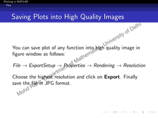
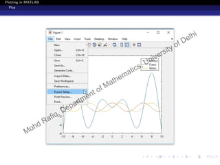
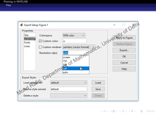
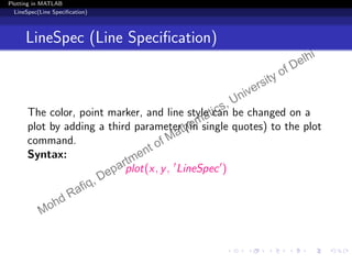
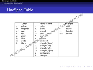
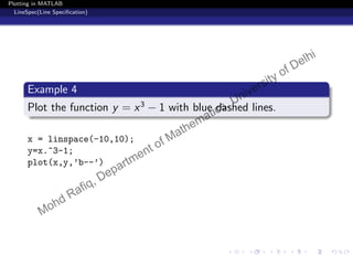
The document discusses various plotting commands and functions in MATLAB. It begins with an outline of topics to be covered, which include the plot command, line specifications, additional plot commands, the fplot command for plotting functions, plotting 2D and 3D functions, and plotting complex numbers. Examples are provided to illustrate how to use the plot command to plot basic functions, combine multiple plots, and customize line properties. Additional commands like hold on and gca are described for combining plots and modifying axis properties. The document provides guidance on plotting, customizing plots, and saving figure files in MATLAB.

1. Plotting in MATLAB
Plotting in MATLAB
By
MOHD RAFIQ
Department of Mathematics
University of Delhi
Delhi
1 / 83

2. Plotting in MATLAB
Outline
1 “Plot” Command
2 / 83
Mohd Rafiq, Department of Mathematics, University of Delhi

3. Plotting in MATLAB
Outline
1 “Plot” Command
2 LineSpec(Line Specification)
2 / 83
Mohd Rafiq, Department of Mathematics, University of Delhi

4. Plotting in MATLAB
Outline
1 “Plot” Command
2 LineSpec(Line Specification)
3 Some Important Additional Commands in Plot
2 / 83
Mohd Rafiq, Department of Mathematics, University of Delhi

5. Plotting in MATLAB
Outline
1 “Plot” Command
2 LineSpec(Line Specification)
3 Some Important Additional Commands in Plot
4 “fplot” Command
2 / 83
Mohd Rafiq, Department of Mathematics, University of Delhi

6. Plotting in MATLAB
Outline
1 “Plot” Command
2 LineSpec(Line Specification)
3 Some Important Additional Commands in Plot
4 “fplot” Command
5 Two variable function( or 3D) plot
2 / 83
Mohd Rafiq, Department of Mathematics, University of Delhi

7. Plotting in MATLAB
Outline
1 “Plot” Command
2 LineSpec(Line Specification)
3 Some Important Additional Commands in Plot
4 “fplot” Command
5 Two variable function( or 3D) plot
6 Plotting complex numbers
2 / 83
Mohd Rafiq, Department of Mathematics, University of Delhi

8. Plotting in MATLAB
Plot
Basic Command for Plotting
Two-dimensional line and symbol plots are created with the
plot command. In its simplest form plot takes two arguments:
plot(xdata, ydata)
where xdata and ydata are vectors containing the data.
3 / 83
Mohd Rafiq, Department of Mathematics, University of Delhi

9. Plotting in MATLAB
Plot
Basic Command for Plotting
Two-dimensional line and symbol plots are created with the
plot command. In its simplest form plot takes two arguments:
plot(xdata, ydata)
where xdata and ydata are vectors containing the data.
Note that xdata and ydata must be the same length and
both must be the same type, i.e., both must be either
row or column vectors.
3 / 83
Mohd Rafiq, Department of Mathematics, University of Delhi

10. Plotting in MATLAB
Plot
Plot Commands
plot
2-D line plot
syntax
plot(X,Y)
plot(X,Y,LineSpec)
plot(X1,Y1,...,Xn,Yn)
plot(X1,Y1,LineSpec1,...,Xn,Yn,LineSpecn)
plot(Y)
plot(Y,LineSpec)
4 / 83
Mohd Rafiq, Department of Mathematics, University of Delhi

11. Plotting in MATLAB
Plot
plot(X,Y) creates a 2-D line plot of the data in Y versus the
corresponding values in X.
plot(X,Y,LineSpec) sets the line style, marker symbol, and color.
plot(X1,Y1,...,Xn,Yn) plots multiple X, Y pairs using the same axes
for all lines.
plot(X1,Y1,LineSpec1,...,Xn,Yn,LineSpecn) sets the line style,
marker type, and color for each line
plot(Y) creates a 2-D line plot of the data in Y versus the index of
each value.
If Y is a vector, then the x-axis scale ranges from 1 to
length(Y).
If Y is a matrix, then the plot function plots the columns of Y
versus their row number. The x-axis scale ranges from 1 to
the number of rows in Y.
If Y is complex, then the plot function plots the imaginary
part of Y versus the real part of Y, such that plot(Y) is
equivalent to plot(real(Y),imag(Y)).
plot(Y,LineSpec) sets the line style, marker symbol, and color. 5 / 83
Mohd Rafiq, Department of Mathematics, University of Delhi

12. Plotting in MATLAB
Plot
Example 1
Plot the function y = sin(x) over the interval [−2π, 2π]
6 / 83
Mohd Rafiq, Department of Mathematics, University of Delhi

13. Plotting in MATLAB
Plot
Example 1
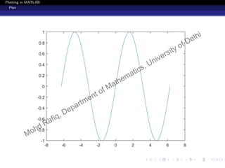
Plot the function y = sin(x) over the interval [−2π, 2π]
x=-2*pi:pi/100:2*pi;
or
x=linspace(-2*pi,2*pi)
y=sin(x);
plot(x,y)
6 / 83
Mohd Rafiq, Department of Mathematics, University of Delhi

14. Plotting in MATLAB
Plot
7 / 83
Mohd Rafiq, Department of Mathematics, University of Delhi

15. Plotting in MATLAB
Plot
Example 2
Plot the functions y1 = sin(x) and y2 = cos(x) over the
interval [−2π, 2π]
8 / 83
Mohd Rafiq, Department of Mathematics, University of Delhi

16. Plotting in MATLAB
Plot
Example 2
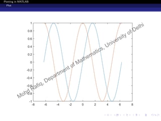
Plot the functions y1 = sin(x) and y2 = cos(x) over the
interval [−2π, 2π]
x=linspace(-2*pi,2*pi);
y1=sin(x);
y2=cos(x);
plot(x,y1,x,y2)
8 / 83
Mohd Rafiq, Department of Mathematics, University of Delhi

17. Plotting in MATLAB
Plot
9 / 83
Mohd Rafiq, Department of Mathematics, University of Delhi

18. Plotting in MATLAB
Plot
Point to Remember
If you are plotting a graph by using any of the operations:
Power (or Exponent)
Multiplications
Division
Then always put a “.”(dot) before these operations.
i.e., type x.^2, x.*y, x./y and 1./x instead of typing
x^2, x*y, x/y and 1/x respectively.
10 / 83
Mohd Rafiq, Department of Mathematics, University of Delhi

19. Plotting in MATLAB
Plot
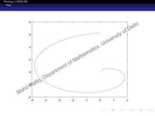
Parametric Plot
Example 3
Plot the parametric curves x = tcos(t) and y = tsin(t)
over[0, 2π].
11 / 83
Mohd Rafiq, Department of Mathematics, University of Delhi

20. Plotting in MATLAB
Plot
Parametric Plot
Example 3
Plot the parametric curves x = tcos(t) and y = tsin(t)
over[0, 2π].
t=linspace(0,2*pi);
x=t.*sin(t);
y=t.*cos(t);
plot(x,y)
11 / 83
Mohd Rafiq, Department of Mathematics, University of Delhi

21. Plotting in MATLAB
Plot
12 / 83
Mohd Rafiq, Department of Mathematics, University of Delhi

22. Plotting in MATLAB
Plot
Saving Plots into High Quality Images
You can save plot of any function into high quality image in
figure window as follows:
File → ExportSetup → Properties → Rendering → Resolution
Choose the highest resolution and click on Export. Finally
save the file in JPG format.
13 / 83
Mohd Rafiq, Department of Mathematics, University of Delhi

23. Plotting in MATLAB
Plot
14 / 83
Mohd Rafiq, Department of Mathematics, University of Delhi

24. Plotting in MATLAB
Plot
15 / 83
Mohd Rafiq, Department of Mathematics, University of Delhi

25. Plotting in MATLAB
LineSpec(Line Specification)
LineSpec (Line Specification)
The color, point marker, and line style can be changed on a
plot by adding a third parameter (in single quotes) to the plot
command.
Syntax:
plot(x, y, LineSpec )
16 / 83
Mohd Rafiq, Department of Mathematics, University of Delhi

26. Plotting in MATLAB
LineSpec(Line Specification)
LineSpec Table
Color Point Marker Line Style
y yellow . point – solid
m magenta o circle : dotted
c cyan x x-mark –. dashdot
r red + plus – – dashed
g green * star
b blue s square
w white d diamond
k black ∨ triangle(down)
∧ triangle(up)
< triangle(left)
> triangle(right)
p pentagram
h hexagon
17 / 83
Mohd Rafiq, Department of Mathematics, University of Delhi

27. Plotting in MATLAB
LineSpec(Line Specification)
Example 4
Plot the function y = x3
− 1 with blue dashed lines.
18 / 83
Mohd Rafiq, Department of Mathematics, University of Delhi

28. Plotting in MATLAB
LineSpec(Line Specification)
Example 4
Plot the function y = x3
− 1 with blue dashed lines.
x = linspace(-10,10);
y=x.^3-1;
plot(x,y,’b--’)
18 / 83
Mohd Rafiq, Department of Mathematics, University of Delhi

29. Plotting in MATLAB
LineSpec(Line Specification)
19 / 83
Mohd Rafiq, Department of Mathematics, University of Delhi

30. Plotting in MATLAB
Some Important Additional Commands in Plot
Combining Two Plots
We can combine two plots by the command
hold on;
20 / 83
Mohd Rafiq, Department of Mathematics, University of Delhi

31. Plotting in MATLAB
Some Important Additional Commands in Plot
Combining Two Plots
We can combine two plots by the command
hold on;
If we apply this to Example 2, then we need to write
x=linspace(-2*pi,2*pi);
y1=sin(x);
y2=cos(x);
plot(x,y1)
hold on;
plot(x,y2)
20 / 83
Mohd Rafiq, Department of Mathematics, University of Delhi

32. Plotting in MATLAB
Some Important Additional Commands in Plot
Displaying the x-axis and y-axis intersecting at
Origin
Note that, by default, the x-axis is at the bottom of the graph
and the y-axis is on the left side. So, if you want to display the
x-axis and y-axis lines so that they cross at the origin point
(0, 0), we add the following command;
21 / 83
Mohd Rafiq, Department of Mathematics, University of Delhi

33. Plotting in MATLAB
Some Important Additional Commands in Plot
Displaying the x-axis and y-axis intersecting at
Origin
Note that, by default, the x-axis is at the bottom of the graph
and the y-axis is on the left side. So, if you want to display the
x-axis and y-axis lines so that they cross at the origin point
(0, 0), we add the following command;
ax=gca;
ax.XAxisLocation=’origin’;
ax.YAxisLocation=’origin’;
Note:
ax=gca; returns the current axes for the current figure
that can be used to access and modify properties of the
axes.
21 / 83
Mohd Rafiq, Department of Mathematics, University of Delhi

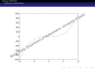
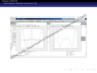
34. Plotting in MATLAB
Some Important Additional Commands in Plot
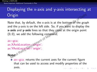
Example 5
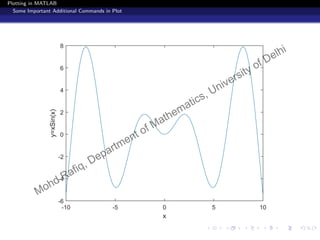
Plot the function y = xSin(x) over the interval [-10,10] and
also show the x-axis and y-axis intersecting at origin.
22 / 83
Mohd Rafiq, Department of Mathematics, University of Delhi

35. Plotting in MATLAB
Some Important Additional Commands in Plot
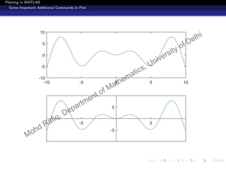
Example 5
Plot the function y = xSin(x) over the interval [-10,10] and
also show the x-axis and y-axis intersecting at origin.
x=linspace(-10,10);
y=x.*sin(x);
plot(x,y)
ax=gca;
ax.XAxisLocation=’origin’;
ax.YAxisLocation=’origin’;
22 / 83
Mohd Rafiq, Department of Mathematics, University of Delhi

36. Plotting in MATLAB
Some Important Additional Commands in Plot
23 / 83
Mohd Rafiq, Department of Mathematics, University of Delhi

37. Plotting in MATLAB
Some Important Additional Commands in Plot
Removing Outline
If you don’t want to show the axes outline, then you can use
the command.
ax.Box=’off’;
24 / 83
Mohd Rafiq, Department of Mathematics, University of Delhi

38. Plotting in MATLAB
Some Important Additional Commands in Plot
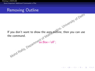
Example 6
Plot the function y = xSin(x) over the interval [-10,10]
without axis outline.
25 / 83
Mohd Rafiq, Department of Mathematics, University of Delhi

39. Plotting in MATLAB
Some Important Additional Commands in Plot
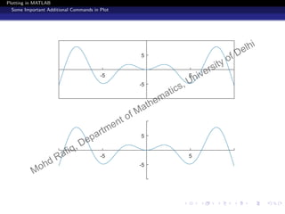
Example 6
Plot the function y = xSin(x) over the interval [-10,10]
without axis outline.
x=linspace(-10,10);
y=x.*sin(x);
plot(x,y)
ax=gca;
ax.XAxisLocation=’origin’;
ax.YAxisLocation=’origin’;
ax.Box=’off’;
25 / 83
Mohd Rafiq, Department of Mathematics, University of Delhi

40. Plotting in MATLAB
Some Important Additional Commands in Plot
26 / 83
Mohd Rafiq, Department of Mathematics, University of Delhi

41. Plotting in MATLAB
Some Important Additional Commands in Plot
Changing the Location of the Tick Marks
We use the following commands for changing the location of
the tick marks on x-axis and y-axis.
ax.XTick=[a1, a2, . . . , am];
ax.YTick=[b1, b2, . . . , bn];
Note: We can replace comma by space in each command.
27 / 83
Mohd Rafiq, Department of Mathematics, University of Delhi

42. Plotting in MATLAB
Some Important Additional Commands in Plot
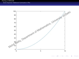
Example 7
Plot the function y = x2
over the interval [0,10] and display
tick marks along the x-axis at the values 0, 5, and 10.
28 / 83
Mohd Rafiq, Department of Mathematics, University of Delhi

43. Plotting in MATLAB
Some Important Additional Commands in Plot
Example 7
Plot the function y = x2
over the interval [0,10] and display
tick marks along the x-axis at the values 0, 5, and 10.
x = linspace(0,10);
y = x.^2;
plot(x,y)
ax=gca;
ax.XTick=[0,5,10];
28 / 83
Mohd Rafiq, Department of Mathematics, University of Delhi

44. Plotting in MATLAB
Some Important Additional Commands in Plot
29 / 83
Mohd Rafiq, Department of Mathematics, University of Delhi

45. Plotting in MATLAB
Some Important Additional Commands in Plot
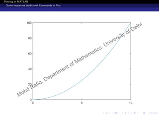
we can also change the location of tick marks on y-axis as
x = linspace(0,10);
y = x.^2;
plot(x,y)
ax=gca;
ax.XTick=[0,5,10];
ax.YTick=[0,20,40,60,80,100];
30 / 83
Mohd Rafiq, Department of Mathematics, University of Delhi

46. Plotting in MATLAB
Some Important Additional Commands in Plot
31 / 83
Mohd Rafiq, Department of Mathematics, University of Delhi

47. Plotting in MATLAB
Some Important Additional Commands in Plot
Labeling the Tick Marks
We can label the tick marks on x-axis and y-axis by the
commands
ax.XTickLabel={’Label1’ , ’Label2’, . . . , ’Labelm’};
ax.YTickLabel={’Label1’ , ’Label2’, . . . , ’Labeln’};
32 / 83
Mohd Rafiq, Department of Mathematics, University of Delhi

48. Plotting in MATLAB
Some Important Additional Commands in Plot
Example 8
Plot the function y = x2
over the interval [0,10] and display
tick marks along the x-axis at the values 0, 5, and 10.Then
specify a label for each tick mark.
33 / 83
Mohd Rafiq, Department of Mathematics, University of Delhi

49. Plotting in MATLAB
Some Important Additional Commands in Plot
Example 8
Plot the function y = x2
over the interval [0,10] and display
tick marks along the x-axis at the values 0, 5, and 10.Then
specify a label for each tick mark.
x = linspace(0,10);
y = x.^2;
plot(x,y)
ax=gca;
ax.XTick=[0,5,10];
ax.XTickLabel={’x=0’,’x=5’,’x=10’};
33 / 83
Mohd Rafiq, Department of Mathematics, University of Delhi

50. Plotting in MATLAB
Some Important Additional Commands in Plot
34 / 83
Mohd Rafiq, Department of Mathematics, University of Delhi

51. Plotting in MATLAB
Some Important Additional Commands in Plot
Upgraded Commands
MATLAB’s latest version (either 2017a or 2017b) has some
new commands and four of them are as follows:
xticks([a1, a2, . . . , am]);
yticks([b1, b2, . . . , bn]);
xticklabels({’Label1’ , ’Label2’, . . . , ’Labelm’});
yticklabels({’Label1’ , ’Label2’, . . . , ’Labeln’});
These commands are upgraded form of previous four
commands.
35 / 83
Mohd Rafiq, Department of Mathematics, University of Delhi

52. Plotting in MATLAB
Some Important Additional Commands in Plot
New Figure Window
If you want to show your plot in a new figure window, then you
can use the command figure just before the command plot.
36 / 83
Mohd Rafiq, Department of Mathematics, University of Delhi

53. Plotting in MATLAB
Some Important Additional Commands in Plot
New Figure Window
If you want to show your plot in a new figure window, then you
can use the command figure just before the command plot.
figure
plot(x,y)
36 / 83
Mohd Rafiq, Department of Mathematics, University of Delhi

54. Plotting in MATLAB
Some Important Additional Commands in Plot
37 / 83
Mohd Rafiq, Department of Mathematics, University of Delhi

55. Plotting in MATLAB
Some Important Additional Commands in Plot
Title
You can give a ”title” to your plot by using the command
title(‘title of plot )
38 / 83
Mohd Rafiq, Department of Mathematics, University of Delhi

56. Plotting in MATLAB
Some Important Additional Commands in Plot
Example 9
Plot the function y = xSin(x) over the interval [-10,10] with
the title “Graph of y=xSin(x)”.
39 / 83
Mohd Rafiq, Department of Mathematics, University of Delhi

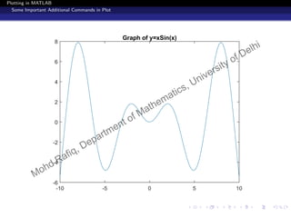
57. Plotting in MATLAB
Some Important Additional Commands in Plot
Example 9
Plot the function y = xSin(x) over the interval [-10,10] with
the title “Graph of y=xSin(x)”.
x=linspace(-10,10);
y=x.*sin(x);
plot(x,y)
title(’Graph of y=xSin(x)’)
39 / 83
Mohd Rafiq, Department of Mathematics, University of Delhi

58. Plotting in MATLAB
Some Important Additional Commands in Plot
40 / 83
Mohd Rafiq, Department of Mathematics, University of Delhi

59. Plotting in MATLAB
Some Important Additional Commands in Plot
Labeling the Axis
You can labels x-axis and y-axis with the following command:
xlabel(‘x − label string )
ylabel(‘y − label string )
41 / 83
Mohd Rafiq, Department of Mathematics, University of Delhi

60. Plotting in MATLAB
Some Important Additional Commands in Plot
Example 10
Plot the function y = xSin(x) over the interval [-10,10] and
also label the axis.
42 / 83
Mohd Rafiq, Department of Mathematics, University of Delhi

61. Plotting in MATLAB
Some Important Additional Commands in Plot
Example 10
Plot the function y = xSin(x) over the interval [-10,10] and
also label the axis.
x=linspace(-10,10);
y=x.*sin(x);
plot(x,y)
xlabel(’x’)
ylabel(’y=xSin(x)’)
42 / 83
Mohd Rafiq, Department of Mathematics, University of Delhi

62. Plotting in MATLAB
Some Important Additional Commands in Plot
43 / 83
Mohd Rafiq, Department of Mathematics, University of Delhi

63. Plotting in MATLAB
Some Important Additional Commands in Plot
Legend
A legend can be added to the plot to identify various curves,
with command:
legend(‘string1 , ‘string2 ..., ‘stringN )
44 / 83
Mohd Rafiq, Department of Mathematics, University of Delhi

64. Plotting in MATLAB
Some Important Additional Commands in Plot
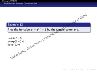
Example 11
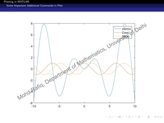
Plot the function xSin(x), Cos(x) and Sin(x) over the interval
[-10,10] and add a legend to for each.
45 / 83
Mohd Rafiq, Department of Mathematics, University of Delhi

65. Plotting in MATLAB
Some Important Additional Commands in Plot
Example 11
Plot the function xSin(x), Cos(x) and Sin(x) over the interval
[-10,10] and add a legend to for each.
x=linspace(-10,10);
y1=x.*sin(x);
y2=cos(x);
y3=sin(x);
plot(x,y1,x,y2,x,y3)
legend(‘xSin(x)’,’Cos(x)’,’Sin(x)’)
45 / 83
Mohd Rafiq, Department of Mathematics, University of Delhi

66. Plotting in MATLAB
Some Important Additional Commands in Plot
46 / 83
Mohd Rafiq, Department of Mathematics, University of Delhi

67. Plotting in MATLAB
Some Important Additional Commands in Plot
Setting the Limit for Axis
The axis command sets the limits for the current axes of the
plot shown, so only the part of the axis that is desirable is
displayed
axis([xmin, xmax, ymin, ymax])
ax.XLim = [xmin, xmax];
ax.YLim = [ymin, ymax];
Note: We can replace comma by space in each command.
47 / 83
Mohd Rafiq, Department of Mathematics, University of Delhi

68. Plotting in MATLAB
Some Important Additional Commands in Plot
Example 12
Plot the function y = e5t
− 1 by the simple command.
48 / 83
Mohd Rafiq, Department of Mathematics, University of Delhi

69. Plotting in MATLAB
Some Important Additional Commands in Plot
Example 12
Plot the function y = e5t
− 1 by the simple command.
t=0:0.01:5;
y=exp(5*t)-1;
plot(t,y)
48 / 83
Mohd Rafiq, Department of Mathematics, University of Delhi

70. Plotting in MATLAB
Some Important Additional Commands in Plot
49 / 83
Mohd Rafiq, Department of Mathematics, University of Delhi

71. Plotting in MATLAB
Some Important Additional Commands in Plot
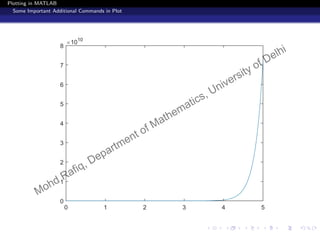
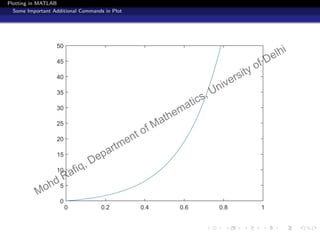
To get a better idea of the initial behavior of the
function, let’s resize the axes. Enter the following
command into the MATLAB command window :
t=0:0.01:5;
y=exp(5*t)-1;
plot(t,y)
axis([0, 1, 0, 50])
50 / 83
Mohd Rafiq, Department of Mathematics, University of Delhi

72. Plotting in MATLAB
Some Important Additional Commands in Plot
51 / 83
Mohd Rafiq, Department of Mathematics, University of Delhi

73. Plotting in MATLAB
Some Important Additional Commands in Plot
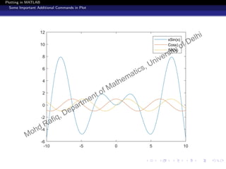
Note that in Example 11, some part of the curve is not
visible because it is covered by the legend. So to
overcome this problem, we can also use axis command.
x=linspace(-10,10);
y1=x.*sin(x);
y2=cos(x);
y3=sin(x);
figure
plot(x,y1,x,y2,x,y3)
legend(’xSin(x)’,’Cosx)’,’Sin(x)’)
ax=gca;
ax.YLim=[-6 12];
52 / 83
Mohd Rafiq, Department of Mathematics, University of Delhi

74. Plotting in MATLAB
Some Important Additional Commands in Plot
53 / 83
Mohd Rafiq, Department of Mathematics, University of Delhi

75. Plotting in MATLAB
Some Important Additional Commands in Plot
Upgraded commands
If you are using MATLAB’s latest version (either 2017a or
2017b) then you can replace the commands ax.XTick and
ax.YTick by the following two commands:
xlim([xmin, xmax]);
ylim([ymin, ymax]);
Note: We can replace comma by space in each command.
54 / 83
Mohd Rafiq, Department of Mathematics, University of Delhi

76. Plotting in MATLAB
fplot command:
fplot command
Use the fplot command to plot either built-in or user defined
functions between specified limits.
fplot(function, interval)
Syntax with Description:
1 fplot(f) plots input f over the default interval [−5 5] for x.
2 fplot(f, x-interval) plots over the specified interval.
Specify the interval as a two-element vector of the form
[xmin xmax].
55 / 83
Mohd Rafiq, Department of Mathematics, University of Delhi

77. Plotting in MATLAB
fplot command:
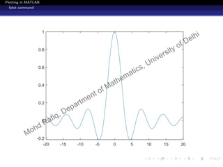
Example 13
Plot the function xSin(x) over the interval [-20,20].
syms x;
fplot(@(x)sin(x)./x,[-20,20]) fplot(sin(x)/x,[-20,20])
or or
f=@(x)sin(x)./x; syms x;
fplot(f,[-20,20]) f(x)=sin(x)/x;
fplot(f,[-20,20])
All commands will give you the same result.
56 / 83
Mohd Rafiq, Department of Mathematics, University of Delhi

78. Plotting in MATLAB
fplot command:
57 / 83
Mohd Rafiq, Department of Mathematics, University of Delhi

79. Plotting in MATLAB
fplot command:
Example 14
Plot the piecewise function
f (x) =
ex
, if − 3 < x < 0
cos x, if 0 < x < 3
58 / 83
Mohd Rafiq, Department of Mathematics, University of Delhi

80. Plotting in MATLAB
fplot command:
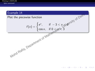
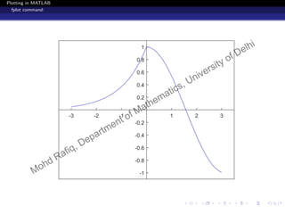
Example 14
Plot the piecewise function
f (x) =
ex
, if − 3 < x < 0
cos x, if 0 < x < 3
syms x;
fplot(exp(x),[-3 0],’b’)
hold on
fplot(cos(x),[0 3],’b’)
axis([-3.5,3.5,-1.1,1.1])
ax=gca;
ax.XAxisLocation=’origin’;
ax.YAxisLocation=’origin’;
58 / 83
Mohd Rafiq, Department of Mathematics, University of Delhi

81. Plotting in MATLAB
fplot command:
59 / 83
Mohd Rafiq, Department of Mathematics, University of Delhi

82. Plotting in MATLAB
fplot command:
Parametric Plot
fplot command is also used to plot 2-D parametric curve.
fplot(xt, yt, interval)
Syntax with Description:
1 fplot(xt,yt) plots xt = x(t) and yt = y(t) over the
default interval of t, which is [–5 5].
2 fplot(xt,yt,t-interval) plots over the specified interval.
Specify the interval as a two-element vector of the form
[tmin tmax].
60 / 83
Mohd Rafiq, Department of Mathematics, University of Delhi

83. Plotting in MATLAB
fplot command:
Example 15
Plot the parametric curve x = cos(t) and y = sin(t).
61 / 83
Mohd Rafiq, Department of Mathematics, University of Delhi

84. Plotting in MATLAB
fplot command:
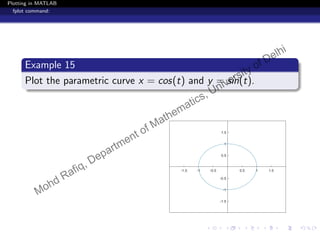
Example 15
Plot the parametric curve x = cos(t) and y = sin(t).
syms t;
fplot(cos(t),sin(t))
axis([-2 2 -2 2])
ax=gca;
ax.XAxisLocation=’origin’;
ax.YAxisLocation=’origin’;
61 / 83
Mohd Rafiq, Department of Mathematics, University of Delhi

85. Plotting in MATLAB
Two variable function( or 3D) plot
Two variable function plot process
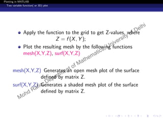
We can plot a function of two variable z = f (x, y) over the
(x, y) region [a, b] × [c, d] as follows:
Steps:
Find grid of (x, y) points as follows
x=a:h1:b;
y=c:h2:d;
[X,Y]=meshgrid(x,y);
Here we have taken grid points step size h1 in the x-direction
and h2 in the y-direction.
62 / 83
Mohd Rafiq, Department of Mathematics, University of Delhi

86. Plotting in MATLAB
Two variable function( or 3D) plot
Apply the function to the grid to get Z-values, where
Z = f (X, Y );
Plot the resulting mesh by the following functions
mesh(X,Y,Z), surf(X,Y,Z)
mesh(X,Y,Z) Generates an open mesh plot of the surface
defined by matrix Z.
surf(X,Y,Z) Generates a shaded mesh plot of the surface
defined by matrix Z.
63 / 83
Mohd Rafiq, Department of Mathematics, University of Delhi

87. Plotting in MATLAB
Two variable function( or 3D) plot
Example 16
Use the meshgrid function to generate matrices x and y.
Create a third matrix, z, and plot its mesh and surf over the
(x, y) region [−2, 2] × [−2, 3], where
z = xe−x2−y2
64 / 83
Mohd Rafiq, Department of Mathematics, University of Delhi

88. Plotting in MATLAB
Two variable function( or 3D) plot
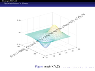
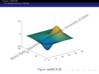
Example 16
Use the meshgrid function to generate matrices x and y.
Create a third matrix, z, and plot its mesh and surf over the
(x, y) region [−2, 2] × [−2, 3], where
z = xe−x2−y2
x=-2:0.1:2;
y=-2:0.1:3;
[X,Y]=meshgrid(x,y);
Z=X.*exp(-X.^2-Y.^2);
figure
mesh(X,Y,Z)
figure
surf(X,Y,Z)
64 / 83
Mohd Rafiq, Department of Mathematics, University of Delhi

89. Plotting in MATLAB
Two variable function( or 3D) plot
Figure: mesh(X,Y,Z)
65 / 83
Mohd Rafiq, Department of Mathematics, University of Delhi

90. Plotting in MATLAB
Two variable function( or 3D) plot
Figure: surf(X,Y,Z)
66 / 83
Mohd Rafiq, Department of Mathematics, University of Delhi

91. Plotting in MATLAB
Two variable function( or 3D) plot
Contour Plot
Syntax:
contour(x, y, z)
67 / 83
Mohd Rafiq, Department of Mathematics, University of Delhi

92. Plotting in MATLAB
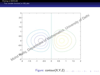
Two variable function( or 3D) plot
Contour Plot
Syntax:
contour(x, y, z)
Example 17
Use the meshgrid function to generate matrices x and y.
Create a third matrix z, and plot its contour over the (x, y)
region [−2, 2] × [−2, 3], where
z = xe−x2−y2
67 / 83
Mohd Rafiq, Department of Mathematics, University of Delhi

93. Plotting in MATLAB
Two variable function( or 3D) plot
Contour Plot
Syntax:
contour(x, y, z)
Example 17
Use the meshgrid function to generate matrices x and y.
Create a third matrix z, and plot its contour over the (x, y)
region [−2, 2] × [−2, 3], where
z = xe−x2−y2
x=-2:0.1:2;
y=-2:0.1:3;
[X,Y]=meshgrid(x,y);
Z=X.*exp(-X.^2-Y.^2);
contour(X,Y,Z)
67 / 83
Mohd Rafiq, Department of Mathematics, University of Delhi

94. Plotting in MATLAB
Two variable function( or 3D) plot
Figure: contour(X,Y,Z)
68 / 83
Mohd Rafiq, Department of Mathematics, University of Delhi

95. Plotting in MATLAB
Two variable function( or 3D) plot
Parametric Plot
Example 18
Plot the following:
x = Sin(t), y = Cos(t), z = t where t ∈ [−10, 10]
69 / 83
Mohd Rafiq, Department of Mathematics, University of Delhi

96. Plotting in MATLAB
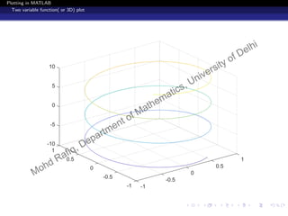
Two variable function( or 3D) plot
Parametric Plot
Example 18
Plot the following:
x = Sin(t), y = Cos(t), z = t where t ∈ [−10, 10]
t=-10:0.1:10;
[T T]=meshgrid(t,t); % or T=meshgrid(t);
x=sin(T);
y=cos(T);
z=T;
mesh(x,y,z)
69 / 83
Mohd Rafiq, Department of Mathematics, University of Delhi

97. Plotting in MATLAB
Two variable function( or 3D) plot
70 / 83
Mohd Rafiq, Department of Mathematics, University of Delhi

98. Plotting in MATLAB
Two variable function( or 3D) plot
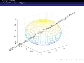
Example 19
The unit sphere centered at the point (0, 0, 1) is given by the
spherical equation
ρ = 2 cos(φ), x = ρ sin(φ) cos(θ), y = ρ sin(φ) sin(θ)
z = ρ cos(φ), where θ ∈ [0, 2π] and φ ∈ [0, π/2]
71 / 83
Mohd Rafiq, Department of Mathematics, University of Delhi

99. Plotting in MATLAB
Two variable function( or 3D) plot
Example 19
The unit sphere centered at the point (0, 0, 1) is given by the
spherical equation
ρ = 2 cos(φ), x = ρ sin(φ) cos(θ), y = ρ sin(φ) sin(θ)
z = ρ cos(φ), where θ ∈ [0, 2π] and φ ∈ [0, π/2]
t=0:0.1:2*pi;
p=0:0.1:pi/2;
[T P]=meshgrid(t,p);
R=2*cos(P);
X=R.*sin(P).*cos(T);
Y=R.*sin(P).*sin(T);
Z=R.*cos(P);
mesh(X,Y,Z)
71 / 83
Mohd Rafiq, Department of Mathematics, University of Delhi

100. Plotting in MATLAB
Two variable function( or 3D) plot
72 / 83
Mohd Rafiq, Department of Mathematics, University of Delhi

101. Plotting in MATLAB
Two variable function( or 3D) plot
f-commands
Just like fplot command in 2D plotting, we have fmesh, fsurf
and fcontour commands in 3D plotting.
Note:
fmesh(f), fsurf(f) and fcontour(f) plot the function
z = f (x, y) over the default interval [-5 5].
Suppose FP denote the fmesh, fsurf and fcontour then
FP(f , xyinterval)
plots over the specified interval. To use the same interval for
both x and y, specify xyinterval as a two-element vector of the
form [min max]. To use different intervals, specify a
four-element vector of the form [xmin xmax ymin ymax].
73 / 83
Mohd Rafiq, Department of Mathematics, University of Delhi

102. Plotting in MATLAB
Two variable function( or 3D) plot
If we apply these commands to Example 16 and 17,then we
will get same plots.
syms x y;
f(x,y)=x.*exp(-x.^2-y.^2);
figure
fmesh(f,[-2 2 -2 3])
figure
fsurf(f,[-2 2 -2 3])
figure
fcontour(f,[-2 2 -2 3])
74 / 83
Mohd Rafiq, Department of Mathematics, University of Delhi

103. Plotting in MATLAB
Plotting complex numbers
Plotting complex numbers
If the input to the plot command is a vector of complex
numbers, the real parts are used as the x-coordinates and the
imaginary parts as the y-coordinates.
i.e., if z is complex, then plot(z) is equivalent to
plot(real(z), imag(z)).
75 / 83
Mohd Rafiq, Department of Mathematics, University of Delhi

104. Plotting in MATLAB
Plotting complex numbers
Plotting complex numbers
If the input to the plot command is a vector of complex
numbers, the real parts are used as the x-coordinates and the
imaginary parts as the y-coordinates.
i.e., if z is complex, then plot(z) is equivalent to
plot(real(z), imag(z)).
Example 20
Define the complex number z = 3 + 2i and plot it as a point
on the complex plane.
z=complex(3,2); z=complex(3,2);
plot(real(z),imag(z),’*’) plot(z,’o’)
75 / 83
Mohd Rafiq, Department of Mathematics, University of Delhi

105. Plotting in MATLAB
Plotting complex numbers
76 / 83
Figure: plot(real(z),imag(z),’*’) Figure: plot(z,’o’)Mohd Rafiq, Department of Mathematics, University of Delhi

106. Plotting in MATLAB
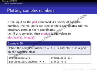
Plotting complex numbers
Point to remember:
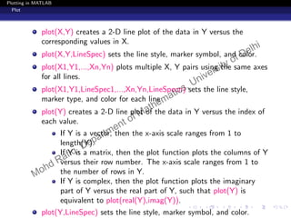
specify a character (’*’, ’+’, ’x’, ’o’, ’.’, etc) to be plotted
at the point.
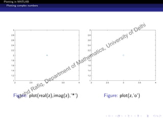
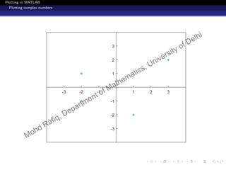
Example 21
Define the complex numbers 3 + 2i, −2 + i, −2 − i, 1 − 2i and
plot them all on the complex plane.
z=[3+2i,-2+1i,-2-1i,1-2i];
plot(z,’*’)
axis([-4 4 -4 4])
ax=gca;
ax.XAxisLocation=’origin’;
ax.YAxisLocation=’origin’;
77 / 83
Mohd Rafiq, Department of Mathematics, University of Delhi

107. Plotting in MATLAB
Plotting complex numbers
78 / 83
Mohd Rafiq, Department of Mathematics, University of Delhi

108. Plotting in MATLAB
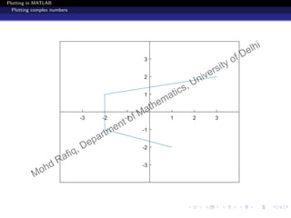
Plotting complex numbers
If we don’t define marker point, then by default MATLAB joins
each point (complex number) in the plot by a line segment.
z=[3+2i,-2+1i,-2-1i,1-2i];
plot(z)
axis([-4 4 -4 4])
ax=gca;
ax.XAxisLocation=’origin’;
ax.YAxisLocation=’origin’;
79 / 83
Mohd Rafiq, Department of Mathematics, University of Delhi

109. Plotting in MATLAB
Plotting complex numbers
80 / 83
Mohd Rafiq, Department of Mathematics, University of Delhi

110. Plotting in MATLAB
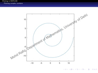
Plotting complex numbers
Example 22
Plot the curve z = teit
for t ∈ [0, 4π].
t=0:0.01:4*pi;
z=t.*exp(i*t); % or z=t.*exp(complex(0,t));
plot(z)
axis([-13 13 -13 13])
81 / 83
Mohd Rafiq, Department of Mathematics, University of Delhi

111. Plotting in MATLAB
Plotting complex numbers
82 / 83
Mohd Rafiq, Department of Mathematics, University of Delhi

112. Plotting in MATLAB
Plotting complex numbers
Thank You...
83 / 83
Mohd Rafiq, Department of Mathematics, University of Delhi