Download as PDF, PPTX


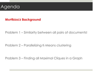
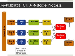

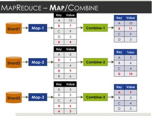
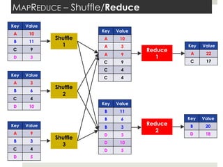

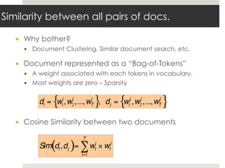
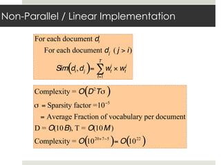
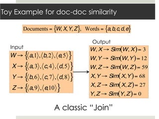
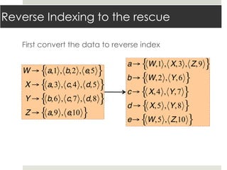
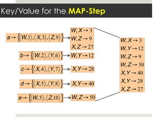
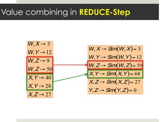
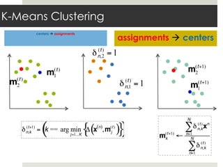
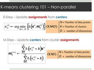
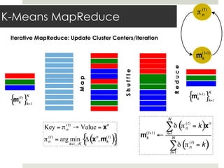
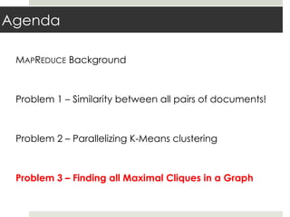
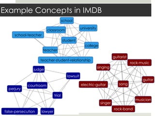
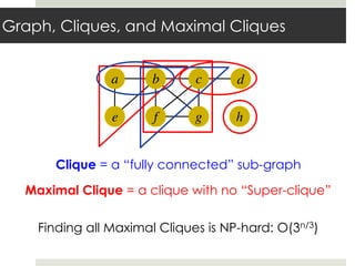

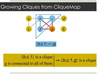
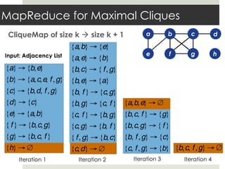
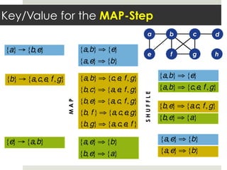
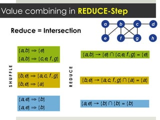
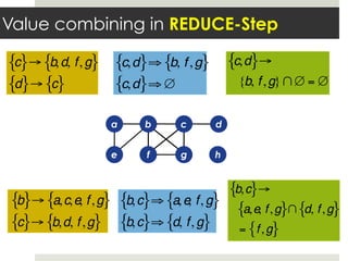
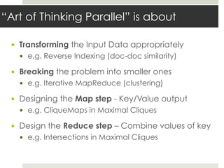

This document discusses parallelizing computation using MapReduce. It begins with an overview of MapReduce and how it works, breaking data into chunks that are processed in parallel by map tasks, and then combining results via reduce tasks. It then provides examples of using MapReduce to solve three problems: 1) calculating similarity between all pairs of documents, 2) parallelizing k-means clustering, and 3) finding all maximal cliques in a graph. For each problem it describes how to define the map and reduce functions to solve the problem in a data-parallel manner using MapReduce.