1. Chapter 2 Supplemental Text Material
S2-1. Models for the Data and the t-Test
The model presented in the text, equation (2-23) is more properly called a means model.
Since the mean is a location parameter, this type of model is also sometimes called a
location model. There are other ways to write the model for a t-test. One possibility is
y
i
j n
ij i ij
i
= + +
=
=
R
S
T
µ τ ε
1 2
1 2
,
, , ,
"
where µ is a parameter that is common to all observed responses (an overall mean) and τi
is a parameter that is unique to the ith factor level. Sometimes we call τi the ith treatment
effect. This model is usually called the effects model.
Since the means model is
y
i
j n
ij i ij
i
= +
=
=
R
S
T
µ ε
1 2
1 2
,
, , ,
"
we see that the ith treatment or factor level mean is µ µ τ
i i
= + ; that is, the mean
response at factor level i is equal to an overall mean plus the effect of the ith factor. We
will use both types of models to represent data from designed experiments. Most of the
time we will work with effects models, because it’s the “traditional” way to present much
of this material. However, there are situations where the means model is useful, and even
more natural.
S2-2. Estimating the Model Parameters
Because models arise naturally in examining data from designed experiments, we
frequently need to estimate the model parameters. We often use the method of least
squares for parameter estimation. This procedure chooses values for the model
parameters that minimize the sum of the squares of the errors εij. We will illustrate this
procedure for the means model. For simplicity, assume that the sample sizes for the two
factor levels are equal; that is n n n
1 2
= = . The least squares function that must be
minimized is
L
y
ij
j
n
i
ij i
j
n
i
=
= −
=
=
=
=
∑
∑
∑
∑
ε
µ
2
1
1
2
2
1
1
2
( )
Now
∂
∂
= −
∂
∂
= −
= =
∑ ∑
L
y
L
y
j
j
n
j
j
n
µ
µ
µ
µ
1
1
1
1
2
2
1
2
2 2
( ) (
and ) and equating these partial derivatives
to zero yields the least squares normal equations
2. n y
n y
j
i
n
j
i
n
µ
µ
1 1
1
2 2
1
=
=
=
=
∑
∑
The solution to these equations gives the least squares estimators of the factor level
means. The solution is
µ µ
1 1 2
= 2
=
y and y ; that is, the sample averages at leach factor
level are the estimators of the factor level means.
This result should be intuitive, as we learn early on in basic statistics courses that the
sample average usually provides a reasonable estimate of the population mean. However,
as we have just seen, this result can be derived easily from a simple location model using
least squares. It also turns out that if we assume that the model errors are normally and
independently distributed, the sample averages are the maximum likelihood estimators
of the factor level means. That is, if the observations are normally distributed, least
squares and maximum likelihood produce exactly the same estimators of the factor level
means. Maximum likelihood is a more general method of parameter estimation that
usually produces parameter estimates that have excellent statistical properties.
We can also apply the method of least squares to the effects model. Assuming equal
sample sizes, the least squares function is
L
y
ij
j
n
i
ij i
j
n
i
=
= − −
=
=
=
=
∑
∑
∑
∑
ε
µ τ
2
1
1
2
2
1
1
2
( )
and the partial derivatives of L with respect to the parameters are
∂
∂
= − −
∂
∂
= − −
∂
∂
= − −
= =
= =
∑ ∑
∑ ∑
L
y
L
y
L
y
ij
j
n
i j
j
n
i
j
j
n
µ
µ τ
τ
µ τ
τ
µ τ
2 2 2
1 1
1
1
1
1
2
2
2
1
2
( ), ( ) (
,and )
Equating these partial derivatives to zero results in the following least squares normal
equations:
2 1 2
1
1
2
1 1
1
2 2
1
n n n y
n n y
n n y
ij
j
n
i
j
j
n
j
j
n
µ τ τ
µ τ
µ τ
+ + =
+ =
+ =
=
=
=
=
∑
∑
∑
∑
Notice that if we add the last two of these normal equations we obtain the first one. That
is, the normal equations are not linearly independent and so they do not have a unique
solution. This has occurred because the effects model is overparameterized. This
3. situation occurs frequently; that is, the effects model for an experiment will always be an
overparameterized model.
One way to deal with this problem is to add another linearly independent equation to the
normal equations. The most common way to do this is to use the equation
τ τ
1 2 0
+ = .
This is, in a sense, an intuitive choice as it essentially defines the factor effects as
deviations from the overall mean µ. If we impose this constraint, the solution to the
normal equations is
, ,
µ
τ
=
= − =
y
y y i
i i 1 2
That is, the overall mean is estimated by the average of all 2n sample observation, while
each individual factor effect is estimated by the difference between the sample average
for that factor level and the average of all observations.
This is not the only possible choice for a linearly independent “constraint” for solving the
normal equations. Another possibility is to simply set the overall mean equal to a
constant, such as for example
µ = 0. This results in the solution
, ,
µ
τ
=
= =
0
1 2
i i
y i
Yet another possibility is
τ 2 0
= , producing the solution
µ
τ
τ
=
= −
=
y
y y
2
1 1
2 0
2
There are an infinite number of possible constraints that could be used to solve the
normal equations. An obvious question is “which solution should we use?” It turns out
that it really doesn’t matter. For each of the three solutions above (indeed for any solution
to the normal equations) we have
, ,
µ µ τ
i i i
y i
= + = = 1 2
That is, the least squares estimator of the mean of the ith factor level will always be the
sample average of the observations at that factor level. So even if we cannot obtain
unique estimates for the parameters in the effects model we can obtain unique estimators
of a function of these parameters that we are interested in. We say that the mean of the
ith factor level is estimable. Any function of the model parameters that can be uniquely
estimated regardless of the constraint selected to solve the normal equations is called an
estimable function. This is discussed in more detail in Chapter 3.
S2-3. A Regression Model Approach to the t-Test
The two-sample t-test can be presented from the viewpoint of a simple linear regression
model. This is a very instructive way to think about the t-test, as it fits in nicely with the
general notion of a factorial experiment with factors at two levels, such as the golf
4. experiment described in Chapter 1. This type of experiment is very important in practice,
and is discussed extensively in subsequent chapters.
In the t-test scenario, we have a factor x with two levels, which we can arbitrarily call
“low” and “high”. We will use x = -1 to denote the low level of this factor and x = +1 to
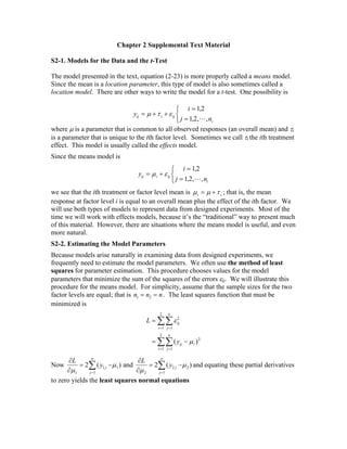
denote the high level of this factor. Figure 2-3.1 below is a scatter plot (from Minitab) of
the portland cement mortar tension bond strength data in Table 2-1 of Chapter 2.
Factor level
Bond
Strength
1.0
0.5
0.0
-0.5
-1.0
17.50
17.25
17.00
16.75
16.50
Figure 2-3.1 Scatter plot of bond strength
We will a simple linear regression model to this data, say
y x
ij ij ij
= + +
β β ε
0 1
where β β
0 and 1 are the intercept and slope, respectively, of the regression line and the
regressor or predictor variable is x j
1 1
= − and x j
2 1
= + . The method of least squares can
be used to estimate the slope and intercept in this model. Assuming that we have equal
sample sizes n for each factor level the least squares normal equations are:
2
2
0
1
1
2
1 2
1
1
1
n y
n y
ij
j
n
i
j
j
n
j
j
n
β
β
=
= −
=
=
= =
∑
∑
∑ ∑y
The solution to these equations is
5. ( )
β
β
0
1 2
1
2
=
= −
y
y y1
Note that the least squares estimator of the intercept is the average of all the observations
from both samples, while the estimator of the slope is one-half of the difference between
the sample averages at the “high” and “low’ levels of the factor x. Below is the output
from the linear regression procedure in Minitab for the tension bond strength data.
Regression Analysis: Bond Strength versus Factor level
The regression equation is
Bond Strength = 16.9 + 0.139 Factor level
Predictor Coef SE Coef T P
Constant 16.9030 0.0636 265.93 0.000
Factor level 0.13900 0.06356 2.19 0.042
S = 0.284253 R-Sq = 21.0% R-Sq(adj) = 16.6%
Analysis of Variance
Source DF SS MS F P
Regression 1 0.38642 0.38642 4.78 0.042
Residual Error 18 1.45440 0.08080
Total 19 1.84082
Notice that the estimate of the slope (given in the column labeled “Coef” and the row
labeled “Factor level” above) is 0.139 2 1
1 1
( ) (17.0420 16.7640)
2 2
y y
= − = − and the
estimate of the intercept is 16.9030. Furthermore, notice that the t-statistic associated
with the slope is equal to 2.19, exactly the same value (apart from sign) that we gave in
the Minitab two-sample t-test output in Table 2-2 in the text. Now in simple linear
regression, the t-test on the slope is actually testing the hypotheses
H
H
0 1
0 1
0
0
:
:
β
β
=
≠
and this is equivalent to testing H0 1 2
:µ µ
= .
It is easy to show that the t-test statistic used for testing that the slope equals zero in
simple linear regression is identical to the usual two-sample t-test. Recall that to test the
above hypotheses in simple linear regression the t-statistic is
6. t
Sxx
0
1
2
=
β
σ
where Sxx = −
=
=
∑
∑ (x x
ij
j
n
i
2
1
1
2
) is the “corrected” sum of squares of the x’s. Now in our
specific problem, x x x
j j
= = − = +
0 1 1,
1 2
, and S n
xx
so = 2 . Therefore, since we have
already observed that the estimate of σ is just Sp,
t
S
y y
S
n
y y
S
n
xx
p p
0
1
2
2 1
2 1
1
2
1
2
2
= =
−
=
−
( )
β
σ
This is the usual two-sample t-test statistic for the case of equal sample sizes.
S2-4. Constructing Normal Probability Plots
While we usually generate normal probability plots using a computer software program,
occasionally we have to construct them by hand. Fortunately, it’s relatively easy to do,
since specialized normal probability plotting paper is widely available. This is just
graph paper with the vertical (or probability) scale arranged so that if we plot the
cumulative normal probabilities (j – 0.5)/n on that scale versus the rank-ordered
observations y(j) a graph equivalent to the computer-generated normal probability plot
will result. The table below shows the calculations for the unmodified portland cement
mortar bond strength data.
j y (j) (j – 0.5)/10 z(j)
1 16.62 0.05 -1.64
2 16.75 0.15 -1.04
3 16.87 0.25 -0.67
4 16.98 0.35 -0.39
5 17.02 0.45 -0.13
6 17.08 0.55 0.13
7 17.12 0.65 0.39
8 17.27 0.75 0.67
9 17.34 0.85 1.04
10 17.37 0.95 1.64
7. Now if we plot the cumulative probabilities from the next-to-last column of this table
versus the rank-ordered observations from the second column on normal probability
paper, we will produce a graph that is identical to the results for the unmodified mortar
formulation that is shown in Figure 2-11 in the text.
A normal probability plot can also be constructed on ordinary graph paper by plotting the
standardized normal z-scores z(j) against the ranked observations, where the standardized
normal z-scores are obtained from
P Z z z
j
n
j j
( ) ( )
.
≤ = =
−
Φ
05
where denotes the standard normal cumulative distribution. For example, if (j –
0.5)/n = 0.05, then
Φ( )
•
Φ( ) . .
zj = zj = −
0 05 164
implies that . The last column of the above
table displays the values of the normal z-scores. Plotting these values against the ranked
observations on ordinary graph paper will produce a normal probability plot equivalent to
the unmodified mortar results in Figure 2-11. As noted in the text, many statistics
computer packages present the normal probability plot this way.
S2-5. More About Checking Assumptions in the t-Test
We noted in the text that a normal probability plot of the observations was an excellent
way to check the normality assumption in the t-test. Instead of plotting the observations,
an alternative is to plot the residuals from the statistical model.
Recall that the means model is
y
i
j n
ij i ij
i
= +
=
=
R
S
T
µ ε
1 2
1 2
,
, , ,
and that the estimates of the parameters (the factor level means) in this model are the
sample averages. Therefore, we could say that the fitted model is
, , , , ,
y y i j n
ij i i
= = =
1 2 1 2
and
That is, an estimate of the ijth observation is just the average of the observations in the ith
factor level. The difference between the observed value of the response and the predicted
(or fitted) value is called a residual, say
e y y i
ij ij i
= − =
, ,
1 2 .
The table below computes the values of the residuals from the portland cement mortar
tension bond strength data.
8. Observation
j
y j
1 e y y
y
j j
j
1 1 1
1 16 76
= −
= − .
y j
2 2 2 2
2 17.04
j j
j
e y y
y
= −
= −
1 16.85 0.09 16.62 -0.42
2 16.40 -0.36 16.75 -0.29
3 17.21 0.45 17.37 0.33
4 16.35 -0.41 17.12 0.08
5 16.52 -0.24 16.98 -0.06
6 17.04 0.28 16.87 -0.17
7 16.96 0.20 17.34 0.30
8 17.15 0.39 17.02 -0.02
9 16.59 -0.17 17.08 0.04
10 16.57 -0.19 17.27 0.23
The figure below is a normal probability plot of these residuals from Minitab.
Residual
Percent
0.50
0.25
0.00
-0.25
-0.50
-0.75
99
95
90
80
70
60
50
40
30
20
10
5
1
Normal Probability Plot of the Residuals
(response is Bond Strength)
9. As noted in section 2-3 above we can compute the t-test statistic using a simple linear
regression model approach. Most regression software packages will also compute a table
or listing of the residuals from the model. The residuals from the Minitab regression
model fit obtained previously are as follows:
Factor Bond
Obs level Strength Fit SE Fit Residual St Resid
1 -1.00 16.8500 16.7640 0.0899 0.0860 0.32
2 -1.00 16.4000 16.7640 0.0899 -0.3640 -1.35
3 -1.00 17.2100 16.7640 0.0899 0.4460 1.65
4 -1.00 16.3500 16.7640 0.0899 -0.4140 -1.54
5 -1.00 16.5200 16.7640 0.0899 -0.2440 -0.90
6 -1.00 17.0400 16.7640 0.0899 0.2760 1.02
7 -1.00 16.9600 16.7640 0.0899 0.1960 0.73
8 -1.00 17.1500 16.7640 0.0899 0.3860 1.43
9 -1.00 16.5900 16.7640 0.0899 -0.1740 -0.65
10 -1.00 16.5700 16.7640 0.0899 -0.1940 -0.72
11 1.00 16.6200 17.0420 0.0899 -0.4220 -1.56
12 1.00 16.7500 17.0420 0.0899 -0.2920 -1.08
13 1.00 17.3700 17.0420 0.0899 0.3280 1.22
14 1.00 17.1200 17.0420 0.0899 0.0780 0.29
15 1.00 16.9800 17.0420 0.0899 -0.0620 -0.23
16 1.00 16.8700 17.0420 0.0899 -0.1720 -0.64
17 1.00 17.3400 17.0420 0.0899 0.2980 1.11
18 1.00 17.0200 17.0420 0.0899 -0.0220 -0.08
19 1.00 17.0800 17.0420 0.0899 0.0380 0.14
20 1.00 17.2700 17.0420 0.0899 0.2280 0.85
The column labeled “Fit” contains the averages of the two samples, computed to four
decimal places. The residuals in the sixth column of this table are the same (apart from
rounding) as we computed manually.
S2-6. Some More Information about the Paired t-Test
The paired t-test examines the difference between two variables and test whether the
mean of those differences differs from zero. In the text we show that the mean of the
differences µd is identical to the difference of the means in two independent samples,
µ µ
1 − 2 . However the variance of the differences is not the same as would be observed if
there were two independent samples. Let d be the sample average of the differences.
Then
V d V y y
V y V y Cov y y
n
( ) ( )
( ) ( ) ( , )
( )
= −
= + −
=
−
1 2
1 2 1
2
2
2 1
σ ρ
2
y2
assuming that both populations have the same variance σ2
and that ρ is the correlation
between the two random variables . The quantity estimates the variance
of the average difference
y1 and S n
d
2
/
d . In many paired experiments a strong positive correlation is
10. expected to exist between because both factor levels have been applied to the
same experimental unit. When there is positive correlation within the pairs, the
denominator for the paired t-test will be smaller than the denominator for the two-sample
or independent t-test. If the two-sample test is applied incorrectly to paired samples, the
procedure will generally understate the significance of the data.
y1 and y2
Note also that while for convenience we have assumed that both populations have the
same variance, the assumption is really unnecessary. The paired t-test is valid when the
variances of the two populations are different.