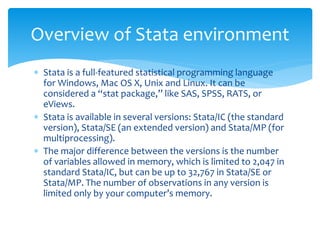
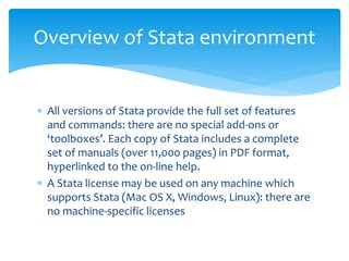
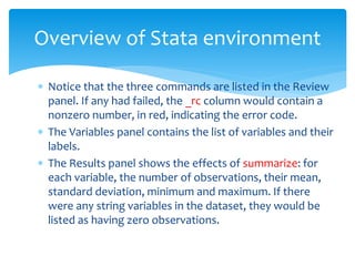
SlideShare a Scribd company logo
1 of 44
Advanced econometrics and Stata
L1-2
Dr. Chunxia Jiang
Business School, University of Aberdeen, UK
Beijing , 17-26 Nov 2019
 Topics and schedule
Sessions plan
10月17日 Evening —
L1-2 Introduction to Econometrics and Stata
10月18日 Evening —
L3-4 Data, simple regression
Morning —
L5-6 Hypothesis testing, Multi-regression , Violation of assumptions
Afternoon Exercises and practice
Morning —
L7-8 Time series models
Evening —
L9-10 Panel data models & Endogeneity
Morning Exercises and practice
Afternoon L11-12 Frontier1 SFA
10月24 Evening L13-14: Frontier2 DEA
10月25日 Evening L15-16 DID
Morning Revision
Afternoon Exam
10月20日
10月19日
10月22日
10月26日
What is Econometrics?
 Economic measurement
 Application of mathematical statistics to economic data to lend
empirical support to the models constructed by mathematical
economics and obtain numerical results.
 Quantitative analysis of actual economic phenomena based on
the concurrent development of theory and observation, related
by appropriate methods of inference.
 The empirical determination of economic laws
 A conjunction of economic theory and actual measurements,
using the theory and techniques of statistical inference as a bridge
pier.
Econometrics
 Try to explain the behaviour of a variable accounting for
factors that might affect the behaviour.
 Example: analyse the determinants of innovative activities
 Objective: What factors affect innovations?
 How do we measure innovations?
 Investment in R&D, number of patents
 What factors do we include as determinants of innovations?
 Skilled workers
 Proximity to universities/research centres
 Access to finance
 Past experience
 Institutional framework
Methodology of econometrics
 Statement of theory or hypothesis
 Model definition
 Data
 Estimation
 Hypothesis testing
 Forecasting
 Policy simulation
Methodology of econometrics :
Statement of theory or hypothesis
 Keynes: marginal propensity to consume (MPC) is greater
than zero but less than 1
 MPC is the rate of change of consumption for a unit change in
income
Methodology of econometrics:
Model definition
 A mathematical model
 Keynes postulated a positive relationship between consumption and
income, but not specify the precise form of the functional relational
relationship between two
Y=β1+β2X 0<β<1 Eq. (1)
Y=consumption, X=income, β1, β2 are parameters - intercept and slope
coefficients; β2 measures MPC
 Eq. (1) is an exact or deterministic relationship, but relationships
between economic variables are generally inexact.
 Eq. (1) is modified to an econometric model
Y=β1+β2X+u Eq. (2)
u is disturbance (error term) that is a random (stochastic) variable
Methodology of econometrics:
Data
 Y=β1+β2X+u Eq. (2)
 To estimate Eq. (2) to obtain the numerical values of
β1, β2, we need data.
 US economy data : personal consumption
expenditure and GDP 1960-2005.
Methodology of econometrics:
Estimation
 Regression analysis we
obtain
 β2 (MPC) is 0.72,
suggesting that for the
sample period 1960-2005
an increase in real income
of one dollar led, on
average, to an increase of
about 72 cents in real
consumption expenditure
t
t X
Y 7218
.
0
5913
.
299
ˆ 


Methodology of econometrics
 Hypothesis testing
 Assuming a good fit of the estimated model, if the estimates
are in accord with the expectations of the theory statistical
inference (hypothesis testing)
 Forecasting
 The chosen model can be used to predict the future value of Y
on the basis of X
 Policy simulation
 The model may be used for control , or policy, purposes.
 i.e., manipulate X to achieve desired Y
Types of Econometrics
 Econometrics
How are data organized?
 Time series data:
 a set of observations on the values that a variable takes at
different times.
 Cross-sectional data:
 Data on one or more variables collected at the same point in
time.
 Pooled or panel data
 Elements of both time series and cross-section data
 Panel data: same cross-sectional unit is surveyed over time
Examples of economic data
 Employment: total number of workers or total
number of hours worked
 Output: total output, industry output
 Skills: number of people with a certain degree
 Capital stocks: physical capital, ICT capital, human
capital
 Import/export/FDI
Examples of financial data
 What sorts of financial variables do we usually want
to explain?
 Prices - stock prices, stock indices, exchange rates
 Returns - stock returns, index returns, interest rates
 Volatility
 Trading volumes
 Corporate finance variables
 Debt issuance, use of hedging instruments
Where do we find the data
 Data sources: primary survey data and secondary published data,
grouped data and non-grouped data
 Macro data: national statistics, world bank, IMF
 Banking data: national central bank, BankScope
 Firm data: datastream,
 Survey to collect first-hand data
 Accuracy of data: selection biases and data quality
 Possible observational errors
 In questionnaire-type survey—non-response
 Sampling
 Aggregate
 Researchers should always keep in mind that the results of
research are only as good as the quality of the data
Elements of economic models:
The basic concepts
 Each model consists of a set of equations. The number of
equations can be various.
 Each equation has a set of variables.
 Each equation has a set of parameters (or coefficients).
 e.g. A very simple macroeconomic model:
Y = C + I + G (1)
C = c0 + c1(Y - T) (2)
T = t0 + t1Y (3)
I = i0 + i1Y + i2R (4)
G = g0 + g1Y (5)
Elements of economic models:
Assumptions
 The economy is a close one. It does not involve any
import or export activities.
 All the equations are linear. Each dependent variable
is exactly explained by the RHS variables.
 The model is 'static' in that all parameters are
assumed to be 'fixed'.
 All the prices and wages are fixed.
 There exists a margin of unused resources.
Types of model:
Single equation model
 This is commonly used for some particular analyses:
 e.g. --- A demand equation for a specific commodity
 Qi
d = f(Income, Pi, Pk)
 Dependent variable: In any single equation, the dependent
variable is always placed on the left hand side (LHS) of the
equation. It is explained or dependent on the expression on the
right hand side. In this case the dependent variable is Qi
d.
 Independent variables: In any single equation, all the
independent variables are placed on the right hand side (RHS) of
the equation. They explain or determine the dependent variable.
They are independent because they do not depend on any other
variables in that equation.
Types of model:
Multi-equation model
Y = C + I + G (1)
C = c0 + c1(Y - T) (2)
T = t0 + t1Y (3)
I = i0 + i1Y + i2R (4)
G = g0 + g1Y (5)
 Dependent variables: Y, C, T, I, G because they are all
on the LHS.
 Independent variables: R.
 Coefficients: c0, c1, t0, t1, i0, i1, i2, g0 and g1.
Simultaneous Equations Models
 A simple example
V = V0 + I (1)
I = i0 + i1R + i2V (2)
Where V is total revenue, V0 is basic revenue of a firm,
I is total investment, and R is interest rate. i0, i1 and i2
are coefficients.
 In the simultaneous equations, dependent variables
are called endogenous and independent variables
exogenous variables.
Simultaneous Equations Models
 How to obtain a reduced form from the structural
form?
 Step I: Let us copy the structural form
V = V0 + I (1)
I = i0 + i1R + i2V (2)
Simultaneous Equations Models
 Step II: Try to express V and I as the functions of exogenous
variables only
 Substitute (2) into (1)
V = V0 + i0 + i1R + i2V
V - i2V = V0 + i0 + i1R
)
3
(
,
1
1
1
1
2
0
1
0
2
1
0
2
2
0
R
V
V
or
R
i
i
V
i
i
i
V


 








Simultaneous Equations Models
 Substitute (1) into (2) and manipulate, we obtain
 Structural and reduced form equations
 Equations (1) and (2) are the structural form equations in
which dependent variables (I and V) can appear on both right
and left-hand sides.
 Equations (3) and (4) are the reduced form equations in
which dependent variables appear only on the left-hand side.
)
4
(
,
1
1
1
2
0
1
0
2
1
0
2
2
2
0
R
V
I
or
R
i
i
V
i
i
i
i
I


 








Questions sheet for lecture 1
1. Examine the following multi-equation system:
C = c0 + c1 Y + c2 R (consumption function with interest rate R)
I = t0 + t1Y + t2R (Investment function with interest rate R)
Y = C + I (definition of GDP as sum of consumption and investment)
(a) List as many as possible the assumptions implied by the model.
(b) List all the dependent variables, the parameters and the independent
variables. Discuss the economic meaning of each parameter in the equation.
2. Derive a reduced form equation for Y from the model in question 1 and
explain what is the marginal effect of R on Y. What do you expect the sizes
and signs of the following parameters a priori: c1, c2, t1 and t2?
L2 An introduction to Stata
Using Stata for data management
and reproducible research
 Stata is a full-featured statistical programming language
for Windows, Mac OS X, Unix and Linux. It can be
considered a “stat package,” like SAS, SPSS, RATS, or
eViews.
 Stata is available in several versions: Stata/IC (the standard
version), Stata/SE (an extended version) and Stata/MP (for
multiprocessing).
 The major difference between the versions is the number
of variables allowed in memory, which is limited to 2,047 in
standard Stata/IC, but can be up to 32,767 in Stata/SE or
Stata/MP. The number of observations in any version is
limited only by your computer’s memory.
Overview of Stata environment
 All versions of Stata provide the full set of features
and commands: there are no special add-ons or
‘toolboxes’. Each copy of Stata includes a complete
set of manuals (over 11,000 pages) in PDF format,
hyperlinked to the on-line help.
 A Stata license may be used on any machine which
supports Stata (Mac OS X, Windows, Linux): there are
no machine-specific licenses
Overview of Stata environment
 Stata is portable, and its developers are committed to
cross-platform compatibility. Stata runs the same way on
Windows, Mac OS X, Unix, and Linux systems
 Perhaps unique among statistical packages, Stata’s binary
data files may be freely copied from one platform to any
other, or even accessed over the Internet from any
machine that runs Stata. You may store Stata’s binary
datafiles on a webserver (HTTP server) and open them on
any machine with access to that server.
Overview of Stata environment
 The Toolbar contains icons that allow you to Open and
Save files, Print results, control Logs, and manipulate
windows. Some very important
 tools allow you to open the Do-File Editor, the Data
Editor and the Data Browser.
 The Data Editor and Data Browser present you with a
spreadsheet-like view of the data, no matter how large
your dataset may be. The Do-File editor, as we will
discuss, allows you to construct a file of Stata commands,
or “do-file”, and execute it in whole or in part from the
editor.
Overview of Stata environment
 There are several panels in the default interface: the Review,
Results, Command, Variables and Properties panels. You may
alter the appearance of any panel using the Preferences-
>General dialog, and make those changes on a temporary or
permanent basis.
 As you might expect, you may type commands in the
Command panel. You may only enter one command in that
panel, so you should not try pasting a list of several commands.
When a command is executed—with or without error—it
appears in the Review panel, and the results of the command
(or an error message) appears in the Results panel. You may
click on any command in the Review panel and it will reappear
in the Command panel, where it may be edited and
resubmitted.
Overview of Stata environment
 Once you have loaded data into the program, the
Variables panel will be populated with information on
each variable, as you can see in the example. That
information includes the variable name, its label (if
any), its type and its format. This is a subset of
information available from the describe command.
 Let’s look at the interface after I have loaded one of
the datasets provided with Stata, uslifeexp, with the
sysuse command and given the describe and
summarize commands:
Overview of Stata environment
 Notice that the three commands are listed in the Review
panel. If any had failed, the _rc column would contain a
nonzero number, in red, indicating the error code.
 The Variables panel contains the list of variables and their
labels.
 The Results panel shows the effects of summarize: for
each variable, the number of observations, their mean,
standard deviation, minimum and maximum. If there
were any string variables in the dataset, they would be
listed as having zero observations.
Overview of Stata environment
 Try it out: type the commands
 sysuse uslifeexp
 describe
 summarize
 Take note of an important design feature of Stata. If you
do not say what to describe or summarize, Stata assumes
you want to perform those commands for every variable in
memory, as shown here. As we shall see, this design
principle holds throughout the program.
Overview of Stata environment
 We may also write a do-file in the do-file editor and execute it. The
 Do-File Editor icon on the Toolbar brings up a window in which we may
 type those same three commands, as well as a few more:
 sysuse uslifeexp
 describe
 summarize
 notes
 // average life expectancy, 1900-1949
 summarize le if year < 1950
 // average life expectancy, 1950-1999
 summarize le if year >= 1950
 After typing those commands into the window, the rightmost icon, with
 tooltip Do, may be used to execute them.
Overview of Stata environment
 In this do-file, I have included the notes command to
display the notes saved with the dataset, and
included two comment lines. There are several styles
of comments available. In this style, anything on a line
following a double slash (//) is ignored.
 You may use the other icons in the Do-File Editor
window to save your do-file, print it, or edit its
contents. You may also select a portion of the file
with the mouse and execute only those commands.
Overview of Stata environment
 Try it out: use the Do-File Editor to save and reopen
the do-file S1.1.do, and run the file.
 Try selecting only those last four lines and run those
commands.
Overview of Stata environment
 The rightmost menu on the menu bar is labeled Help. From
that menu, you can search for help on any command or
feature. The Help Browser, which opens in a Viewer
window, provides hyperlinks, in blue, to additional help
pages. At the foot of each help screen, there are hyperlinks
to the full manuals, which are accessible in PDF format. The
links will take you directly to the appropriate page of the
manual.
 You may also search for help at the command line with
help command. But what if you don’t know the exact
command name? Then you may use the search command,
which may be followed by one or several words.
Overview of Stata environment
 Results from search are presented in a Viewer window.
Those commands will present results from a keyword
database and from the Internet: for instance, FAQs from
the Stata website, articles in the Stata Journal and Stata
Technical Bulletin, and downloadable routines from the
SSC Archive (about which more later) and user sites.
 Try it out: when you are connected to the Internet, type
the command search baum, au and then try search baum
 Note the hyperlinks that appear on URLs for the books and
journal articles, and on the individual software packages
(e.g., st0030_3, archlm).
Overview of Stata environment
 One of Stata’s great strengths is that it can be updated
over the Internet. Stata is actually a web browser, so it
may contact Stata’s web server and enquire whether there
are more recent versions of either Stata’s executable (the
kernel) or the ado-files. This enables Stata’s developers to
distribute bug fixes, enhancements to existing commands,
and even entirely new commands during the lifetime of a
given major release (including ‘dot-releases’ such as Stata
14.1).
 Updates during the life of the version you own are free.
You need only have a licensed copy of Stata and access to
the Internet (which may be by proxy server) to check for
and, if desired, download the updates.
Overview of Stata environment
 Another advantage of the command-line driven
environment involves extensibility: the continual
expansion of Stata’s capabilities. A command, to
Stata, is a verb instructing the program to perform
some action.
 Commands may be “built in” commands—those
elements so frequently used that they have been
coded into the “Stata kernel.” A relatively small
fraction of the total number of official Stata
commands are built in, but they are used very heavily.
Overview of Stata environment
 If Stata’s developers tomorrow wrote a new
command named “foobar”, they would make two
files available on their web site: foobar.ado (the ado-
file code) and foobar.sthlp (the associated help file).
Both are ordinary, readable ASCII text files. These files
should be produced in a text editor, not a word
processing program.
Overview of Stata environment
 The importance of this program design goes far
beyond the limits of official Stata.
 You may acquire new Stata commands from a
number of web sites. The Stata Journal (SJ), a
quarterly peer-reviewed journal, is the primary
method for distributing user contributions. Between
1991 and 2001, the Stata Technical Bulletin played this
role, and a complete set of issues of the STB are
available on line at the Stata website.
Overview of Stata environment
 The importance of all this is that Stata is infinitely
extensible. Any ado-file on your adopath is a full-
fledged Stata command. Stata’s capabilities thus
extend far beyond the official, supported features
described in the Stata manual to a vast array of
additional tools.
Overview of Stata environment
 Create our own list…
Command focus

More Related Content

Similar to Advanced Econometrics L1-2.pptx

Econometrics_1.pptx
Econometrics_1.pptxEconometrics_1.pptx
Econometrics_1.pptxSoumiliBera2
 
Course Title: Introduction to Machine Learning, Chapter 2- Supervised Learning
Course Title: Introduction to Machine Learning,  Chapter 2- Supervised LearningCourse Title: Introduction to Machine Learning,  Chapter 2- Supervised Learning
Course Title: Introduction to Machine Learning, Chapter 2- Supervised LearningShumet Tadesse
 
1.1.Introduction Econometrics.pptx
1.1.Introduction Econometrics.pptx1.1.Introduction Econometrics.pptx
1.1.Introduction Econometrics.pptxAyushKumar685245
 
Chapter one: Introduction to Econometrics.ppt
Chapter one: Introduction to Econometrics.pptChapter one: Introduction to Econometrics.ppt
Chapter one: Introduction to Econometrics.pptaschalew shiferaw
 
Estimating Financial Frictions under Learning
Estimating Financial Frictions under LearningEstimating Financial Frictions under Learning
Estimating Financial Frictions under LearningGRAPE
 
Intro to econometrics
Intro to econometricsIntro to econometrics
Intro to econometricsGaetan Lion
 
Managerial Economics - Demand Estimation (regression analysis)
Managerial Economics - Demand Estimation (regression analysis)Managerial Economics - Demand Estimation (regression analysis)
Managerial Economics - Demand Estimation (regression analysis)JooneEltanal
 
Multiple Regression.ppt
Multiple Regression.pptMultiple Regression.ppt
Multiple Regression.pptTanyaWadhwani4
 
EMPIRICAL PROJECTObjective to help students put in practice w.docx
EMPIRICAL PROJECTObjective  to help students put in practice w.docxEMPIRICAL PROJECTObjective  to help students put in practice w.docx
EMPIRICAL PROJECTObjective to help students put in practice w.docxSALU18
 
project planning demand Estimation II.pptx
project planning demand Estimation  II.pptxproject planning demand Estimation  II.pptx
project planning demand Estimation II.pptxtadegebreyesus
 
Polynomial regression model of making cost prediction in mixed cost analysis
Polynomial regression model of making cost prediction in mixed cost analysisPolynomial regression model of making cost prediction in mixed cost analysis
Polynomial regression model of making cost prediction in mixed cost analysisAlexander Decker
 
11.polynomial regression model of making cost prediction in mixed cost analysis
11.polynomial regression model of making cost prediction in mixed cost analysis11.polynomial regression model of making cost prediction in mixed cost analysis
11.polynomial regression model of making cost prediction in mixed cost analysisAlexander Decker
 
Multivariate analysis of the impact of the commercial banks on the economic g...
Multivariate analysis of the impact of the commercial banks on the economic g...Multivariate analysis of the impact of the commercial banks on the economic g...
Multivariate analysis of the impact of the commercial banks on the economic g...Alexander Decker
 
Data Analysison Regression
Data Analysison RegressionData Analysison Regression
Data Analysison Regressionjamuga gitulho
 
Different Level of Financial Development and Individual’s Decision Regarding ...
Different Level of Financial Development and Individual’s Decision Regarding ...Different Level of Financial Development and Individual’s Decision Regarding ...
Different Level of Financial Development and Individual’s Decision Regarding ...Associate Professor in VSB Coimbatore
 

Similar to Advanced Econometrics L1-2.pptx (20)

Econometrics_1.pptx
Econometrics_1.pptxEconometrics_1.pptx
Econometrics_1.pptx
 
Course Title: Introduction to Machine Learning, Chapter 2- Supervised Learning
Course Title: Introduction to Machine Learning,  Chapter 2- Supervised LearningCourse Title: Introduction to Machine Learning,  Chapter 2- Supervised Learning
Course Title: Introduction to Machine Learning, Chapter 2- Supervised Learning
 
Ekonometrika
EkonometrikaEkonometrika
Ekonometrika
 
1.1.Introduction Econometrics.pptx
1.1.Introduction Econometrics.pptx1.1.Introduction Econometrics.pptx
1.1.Introduction Econometrics.pptx
 
MModule 1 ppt.pptx
MModule 1 ppt.pptxMModule 1 ppt.pptx
MModule 1 ppt.pptx
 
Chapter one: Introduction to Econometrics.ppt
Chapter one: Introduction to Econometrics.pptChapter one: Introduction to Econometrics.ppt
Chapter one: Introduction to Econometrics.ppt
 
Estimating Financial Frictions under Learning
Estimating Financial Frictions under LearningEstimating Financial Frictions under Learning
Estimating Financial Frictions under Learning
 
Intro to econometrics
Intro to econometricsIntro to econometrics
Intro to econometrics
 
Managerial Economics - Demand Estimation (regression analysis)
Managerial Economics - Demand Estimation (regression analysis)Managerial Economics - Demand Estimation (regression analysis)
Managerial Economics - Demand Estimation (regression analysis)
 
Labour Productivity Dynamics Regularities Analyses by Manufacturing in Europe...
Labour Productivity Dynamics Regularities Analyses by Manufacturing in Europe...Labour Productivity Dynamics Regularities Analyses by Manufacturing in Europe...
Labour Productivity Dynamics Regularities Analyses by Manufacturing in Europe...
 
Multiple Regression.ppt
Multiple Regression.pptMultiple Regression.ppt
Multiple Regression.ppt
 
EMPIRICAL PROJECTObjective to help students put in practice w.docx
EMPIRICAL PROJECTObjective  to help students put in practice w.docxEMPIRICAL PROJECTObjective  to help students put in practice w.docx
EMPIRICAL PROJECTObjective to help students put in practice w.docx
 
Econ ch 6
Econ ch 6Econ ch 6
Econ ch 6
 
project planning demand Estimation II.pptx
project planning demand Estimation  II.pptxproject planning demand Estimation  II.pptx
project planning demand Estimation II.pptx
 
Polynomial regression model of making cost prediction in mixed cost analysis
Polynomial regression model of making cost prediction in mixed cost analysisPolynomial regression model of making cost prediction in mixed cost analysis
Polynomial regression model of making cost prediction in mixed cost analysis
 
11.polynomial regression model of making cost prediction in mixed cost analysis
11.polynomial regression model of making cost prediction in mixed cost analysis11.polynomial regression model of making cost prediction in mixed cost analysis
11.polynomial regression model of making cost prediction in mixed cost analysis
 
Multivariate analysis of the impact of the commercial banks on the economic g...
Multivariate analysis of the impact of the commercial banks on the economic g...Multivariate analysis of the impact of the commercial banks on the economic g...
Multivariate analysis of the impact of the commercial banks on the economic g...
 
Forecasting
ForecastingForecasting
Forecasting
 
Data Analysison Regression
Data Analysison RegressionData Analysison Regression
Data Analysison Regression
 
Different Level of Financial Development and Individual’s Decision Regarding ...
Different Level of Financial Development and Individual’s Decision Regarding ...Different Level of Financial Development and Individual’s Decision Regarding ...
Different Level of Financial Development and Individual’s Decision Regarding ...
 

More from akashayosha

Capital Market Responses to Environmental performance.pptx
Capital Market Responses to Environmental performance.pptxCapital Market Responses to Environmental performance.pptx
Capital Market Responses to Environmental performance.pptxakashayosha
 
Advanced Microeconomics Presentation.pptx
Advanced Microeconomics Presentation.pptxAdvanced Microeconomics Presentation.pptx
Advanced Microeconomics Presentation.pptxakashayosha
 
Lab practice session.pptx
Lab practice session.pptxLab practice session.pptx
Lab practice session.pptxakashayosha
 
Advanced Econometrics L13-14.pptx
Advanced Econometrics L13-14.pptxAdvanced Econometrics L13-14.pptx
Advanced Econometrics L13-14.pptxakashayosha
 
Advanced Econometrics L11- 12.pptx
Advanced Econometrics L11- 12.pptxAdvanced Econometrics L11- 12.pptx
Advanced Econometrics L11- 12.pptxakashayosha
 
Advanced Econometrics L10.pptx
Advanced Econometrics L10.pptxAdvanced Econometrics L10.pptx
Advanced Econometrics L10.pptxakashayosha
 
Advanced Econometrics L9.pptx
Advanced Econometrics L9.pptxAdvanced Econometrics L9.pptx
Advanced Econometrics L9.pptxakashayosha
 
Advanced Econometrics L7-8.pptx
Advanced Econometrics L7-8.pptxAdvanced Econometrics L7-8.pptx
Advanced Econometrics L7-8.pptxakashayosha
 
Advanced Econometrics L5-6.pptx
Advanced Econometrics L5-6.pptxAdvanced Econometrics L5-6.pptx
Advanced Econometrics L5-6.pptxakashayosha
 

More from akashayosha (16)

HSK1-L6.pptx
HSK1-L6.pptxHSK1-L6.pptx
HSK1-L6.pptx
 
HSK1-L5.pptx
HSK1-L5.pptxHSK1-L5.pptx
HSK1-L5.pptx
 
HSK1-L4.pptx
HSK1-L4.pptxHSK1-L4.pptx
HSK1-L4.pptx
 
HSK1-L3.pptx
HSK1-L3.pptxHSK1-L3.pptx
HSK1-L3.pptx
 
HSK1-L2.pptx
HSK1-L2.pptxHSK1-L2.pptx
HSK1-L2.pptx
 
HSK1-L1.pptx
HSK1-L1.pptxHSK1-L1.pptx
HSK1-L1.pptx
 
Capital Market Responses to Environmental performance.pptx
Capital Market Responses to Environmental performance.pptxCapital Market Responses to Environmental performance.pptx
Capital Market Responses to Environmental performance.pptx
 
Advanced Microeconomics Presentation.pptx
Advanced Microeconomics Presentation.pptxAdvanced Microeconomics Presentation.pptx
Advanced Microeconomics Presentation.pptx
 
Lab practice session.pptx
Lab practice session.pptxLab practice session.pptx
Lab practice session.pptx
 
Exercises.pptx
Exercises.pptxExercises.pptx
Exercises.pptx
 
Advanced Econometrics L13-14.pptx
Advanced Econometrics L13-14.pptxAdvanced Econometrics L13-14.pptx
Advanced Econometrics L13-14.pptx
 
Advanced Econometrics L11- 12.pptx
Advanced Econometrics L11- 12.pptxAdvanced Econometrics L11- 12.pptx
Advanced Econometrics L11- 12.pptx
 
Advanced Econometrics L10.pptx
Advanced Econometrics L10.pptxAdvanced Econometrics L10.pptx
Advanced Econometrics L10.pptx
 
Advanced Econometrics L9.pptx
Advanced Econometrics L9.pptxAdvanced Econometrics L9.pptx
Advanced Econometrics L9.pptx
 
Advanced Econometrics L7-8.pptx
Advanced Econometrics L7-8.pptxAdvanced Econometrics L7-8.pptx
Advanced Econometrics L7-8.pptx
 
Advanced Econometrics L5-6.pptx
Advanced Econometrics L5-6.pptxAdvanced Econometrics L5-6.pptx
Advanced Econometrics L5-6.pptx
 

Recently uploaded

Instant Issue Debit Cards - High School Spirit
Instant Issue Debit Cards - High School SpiritInstant Issue Debit Cards - High School Spirit
Instant Issue Debit Cards - High School Spiritegoetzinger
 
Andheri Call Girls In 9825968104 Mumbai Hot Models
Andheri Call Girls In 9825968104 Mumbai Hot ModelsAndheri Call Girls In 9825968104 Mumbai Hot Models
Andheri Call Girls In 9825968104 Mumbai Hot Modelshematsharma006
 
20240429 Calibre April 2024 Investor Presentation.pdf
20240429 Calibre April 2024 Investor Presentation.pdf20240429 Calibre April 2024 Investor Presentation.pdf
20240429 Calibre April 2024 Investor Presentation.pdfAdnet Communications
 
VIP Kolkata Call Girl Serampore 👉 8250192130 Available With Room
VIP Kolkata Call Girl Serampore 👉 8250192130  Available With RoomVIP Kolkata Call Girl Serampore 👉 8250192130  Available With Room
VIP Kolkata Call Girl Serampore 👉 8250192130 Available With Roomdivyansh0kumar0
 
Quarter 4- Module 3 Principles of Marketing
Quarter 4- Module 3 Principles of MarketingQuarter 4- Module 3 Principles of Marketing
Quarter 4- Module 3 Principles of MarketingMaristelaRamos12
 
Q3 2024 Earnings Conference Call and Webcast Slides
Q3 2024 Earnings Conference Call and Webcast SlidesQ3 2024 Earnings Conference Call and Webcast Slides
Q3 2024 Earnings Conference Call and Webcast SlidesMarketing847413
 
Chapter 2.ppt of macroeconomics by mankiw 9th edition
Chapter 2.ppt of macroeconomics by mankiw 9th editionChapter 2.ppt of macroeconomics by mankiw 9th edition
Chapter 2.ppt of macroeconomics by mankiw 9th editionMuhammadHusnain82237
 
Independent Call Girl Number in Kurla Mumbai📲 Pooja Nehwal 9892124323 💞 Full ...
Independent Call Girl Number in Kurla Mumbai📲 Pooja Nehwal 9892124323 💞 Full ...Independent Call Girl Number in Kurla Mumbai📲 Pooja Nehwal 9892124323 💞 Full ...
Independent Call Girl Number in Kurla Mumbai📲 Pooja Nehwal 9892124323 💞 Full ...Pooja Nehwal
 
20240417-Calibre-April-2024-Investor-Presentation.pdf
20240417-Calibre-April-2024-Investor-Presentation.pdf20240417-Calibre-April-2024-Investor-Presentation.pdf
20240417-Calibre-April-2024-Investor-Presentation.pdfAdnet Communications
 
VIP Call Girls in Saharanpur Aarohi 8250192130 Independent Escort Service Sah...
VIP Call Girls in Saharanpur Aarohi 8250192130 Independent Escort Service Sah...VIP Call Girls in Saharanpur Aarohi 8250192130 Independent Escort Service Sah...
VIP Call Girls in Saharanpur Aarohi 8250192130 Independent Escort Service Sah...Suhani Kapoor
 
Independent Lucknow Call Girls 8923113531WhatsApp Lucknow Call Girls make you...
Independent Lucknow Call Girls 8923113531WhatsApp Lucknow Call Girls make you...Independent Lucknow Call Girls 8923113531WhatsApp Lucknow Call Girls make you...
Independent Lucknow Call Girls 8923113531WhatsApp Lucknow Call Girls make you...makika9823
 
Best VIP Call Girls Noida Sector 18 Call Me: 8448380779
Best VIP Call Girls Noida Sector 18 Call Me: 8448380779Best VIP Call Girls Noida Sector 18 Call Me: 8448380779
Best VIP Call Girls Noida Sector 18 Call Me: 8448380779Delhi Call girls
 
VIP High Class Call Girls Saharanpur Anushka 8250192130 Independent Escort Se...
VIP High Class Call Girls Saharanpur Anushka 8250192130 Independent Escort Se...VIP High Class Call Girls Saharanpur Anushka 8250192130 Independent Escort Se...
VIP High Class Call Girls Saharanpur Anushka 8250192130 Independent Escort Se...Suhani Kapoor
 
Bladex Earnings Call Presentation 1Q2024
Bladex Earnings Call Presentation 1Q2024Bladex Earnings Call Presentation 1Q2024
Bladex Earnings Call Presentation 1Q2024Bladex
 
VVIP Pune Call Girls Katraj (7001035870) Pune Escorts Nearby with Complete Sa...
VVIP Pune Call Girls Katraj (7001035870) Pune Escorts Nearby with Complete Sa...VVIP Pune Call Girls Katraj (7001035870) Pune Escorts Nearby with Complete Sa...
VVIP Pune Call Girls Katraj (7001035870) Pune Escorts Nearby with Complete Sa...Call Girls in Nagpur High Profile
 
VIP Call Girls LB Nagar ( Hyderabad ) Phone 8250192130 | ₹5k To 25k With Room...
VIP Call Girls LB Nagar ( Hyderabad ) Phone 8250192130 | ₹5k To 25k With Room...VIP Call Girls LB Nagar ( Hyderabad ) Phone 8250192130 | ₹5k To 25k With Room...
VIP Call Girls LB Nagar ( Hyderabad ) Phone 8250192130 | ₹5k To 25k With Room...Suhani Kapoor
 
Shrambal_Distributors_Newsletter_Apr-2024 (1).pdf
Shrambal_Distributors_Newsletter_Apr-2024 (1).pdfShrambal_Distributors_Newsletter_Apr-2024 (1).pdf
Shrambal_Distributors_Newsletter_Apr-2024 (1).pdfvikashdidwania1
 
fca-bsps-decision-letter-redacted (1).pdf
fca-bsps-decision-letter-redacted (1).pdffca-bsps-decision-letter-redacted (1).pdf
fca-bsps-decision-letter-redacted (1).pdfHenry Tapper
 
call girls in Nand Nagri (DELHI) 🔝 >༒9953330565🔝 genuine Escort Service 🔝✔️✔️
call girls in  Nand Nagri (DELHI) 🔝 >༒9953330565🔝 genuine Escort Service 🔝✔️✔️call girls in  Nand Nagri (DELHI) 🔝 >༒9953330565🔝 genuine Escort Service 🔝✔️✔️
call girls in Nand Nagri (DELHI) 🔝 >༒9953330565🔝 genuine Escort Service 🔝✔️✔️9953056974 Low Rate Call Girls In Saket, Delhi NCR
 

Recently uploaded (20)

Instant Issue Debit Cards - High School Spirit
Instant Issue Debit Cards - High School SpiritInstant Issue Debit Cards - High School Spirit
Instant Issue Debit Cards - High School Spirit
 
Andheri Call Girls In 9825968104 Mumbai Hot Models
Andheri Call Girls In 9825968104 Mumbai Hot ModelsAndheri Call Girls In 9825968104 Mumbai Hot Models
Andheri Call Girls In 9825968104 Mumbai Hot Models
 
20240429 Calibre April 2024 Investor Presentation.pdf
20240429 Calibre April 2024 Investor Presentation.pdf20240429 Calibre April 2024 Investor Presentation.pdf
20240429 Calibre April 2024 Investor Presentation.pdf
 
VIP Kolkata Call Girl Serampore 👉 8250192130 Available With Room
VIP Kolkata Call Girl Serampore 👉 8250192130  Available With RoomVIP Kolkata Call Girl Serampore 👉 8250192130  Available With Room
VIP Kolkata Call Girl Serampore 👉 8250192130 Available With Room
 
Quarter 4- Module 3 Principles of Marketing
Quarter 4- Module 3 Principles of MarketingQuarter 4- Module 3 Principles of Marketing
Quarter 4- Module 3 Principles of Marketing
 
Q3 2024 Earnings Conference Call and Webcast Slides
Q3 2024 Earnings Conference Call and Webcast SlidesQ3 2024 Earnings Conference Call and Webcast Slides
Q3 2024 Earnings Conference Call and Webcast Slides
 
Chapter 2.ppt of macroeconomics by mankiw 9th edition
Chapter 2.ppt of macroeconomics by mankiw 9th editionChapter 2.ppt of macroeconomics by mankiw 9th edition
Chapter 2.ppt of macroeconomics by mankiw 9th edition
 
Independent Call Girl Number in Kurla Mumbai📲 Pooja Nehwal 9892124323 💞 Full ...
Independent Call Girl Number in Kurla Mumbai📲 Pooja Nehwal 9892124323 💞 Full ...Independent Call Girl Number in Kurla Mumbai📲 Pooja Nehwal 9892124323 💞 Full ...
Independent Call Girl Number in Kurla Mumbai📲 Pooja Nehwal 9892124323 💞 Full ...
 
🔝+919953056974 🔝young Delhi Escort service Pusa Road
🔝+919953056974 🔝young Delhi Escort service Pusa Road🔝+919953056974 🔝young Delhi Escort service Pusa Road
🔝+919953056974 🔝young Delhi Escort service Pusa Road
 
20240417-Calibre-April-2024-Investor-Presentation.pdf
20240417-Calibre-April-2024-Investor-Presentation.pdf20240417-Calibre-April-2024-Investor-Presentation.pdf
20240417-Calibre-April-2024-Investor-Presentation.pdf
 
VIP Call Girls in Saharanpur Aarohi 8250192130 Independent Escort Service Sah...
VIP Call Girls in Saharanpur Aarohi 8250192130 Independent Escort Service Sah...VIP Call Girls in Saharanpur Aarohi 8250192130 Independent Escort Service Sah...
VIP Call Girls in Saharanpur Aarohi 8250192130 Independent Escort Service Sah...
 
Independent Lucknow Call Girls 8923113531WhatsApp Lucknow Call Girls make you...
Independent Lucknow Call Girls 8923113531WhatsApp Lucknow Call Girls make you...Independent Lucknow Call Girls 8923113531WhatsApp Lucknow Call Girls make you...
Independent Lucknow Call Girls 8923113531WhatsApp Lucknow Call Girls make you...
 
Best VIP Call Girls Noida Sector 18 Call Me: 8448380779
Best VIP Call Girls Noida Sector 18 Call Me: 8448380779Best VIP Call Girls Noida Sector 18 Call Me: 8448380779
Best VIP Call Girls Noida Sector 18 Call Me: 8448380779
 
VIP High Class Call Girls Saharanpur Anushka 8250192130 Independent Escort Se...
VIP High Class Call Girls Saharanpur Anushka 8250192130 Independent Escort Se...VIP High Class Call Girls Saharanpur Anushka 8250192130 Independent Escort Se...
VIP High Class Call Girls Saharanpur Anushka 8250192130 Independent Escort Se...
 
Bladex Earnings Call Presentation 1Q2024
Bladex Earnings Call Presentation 1Q2024Bladex Earnings Call Presentation 1Q2024
Bladex Earnings Call Presentation 1Q2024
 
VVIP Pune Call Girls Katraj (7001035870) Pune Escorts Nearby with Complete Sa...
VVIP Pune Call Girls Katraj (7001035870) Pune Escorts Nearby with Complete Sa...VVIP Pune Call Girls Katraj (7001035870) Pune Escorts Nearby with Complete Sa...
VVIP Pune Call Girls Katraj (7001035870) Pune Escorts Nearby with Complete Sa...
 
VIP Call Girls LB Nagar ( Hyderabad ) Phone 8250192130 | ₹5k To 25k With Room...
VIP Call Girls LB Nagar ( Hyderabad ) Phone 8250192130 | ₹5k To 25k With Room...VIP Call Girls LB Nagar ( Hyderabad ) Phone 8250192130 | ₹5k To 25k With Room...
VIP Call Girls LB Nagar ( Hyderabad ) Phone 8250192130 | ₹5k To 25k With Room...
 
Shrambal_Distributors_Newsletter_Apr-2024 (1).pdf
Shrambal_Distributors_Newsletter_Apr-2024 (1).pdfShrambal_Distributors_Newsletter_Apr-2024 (1).pdf
Shrambal_Distributors_Newsletter_Apr-2024 (1).pdf
 
fca-bsps-decision-letter-redacted (1).pdf
fca-bsps-decision-letter-redacted (1).pdffca-bsps-decision-letter-redacted (1).pdf
fca-bsps-decision-letter-redacted (1).pdf
 
call girls in Nand Nagri (DELHI) 🔝 >༒9953330565🔝 genuine Escort Service 🔝✔️✔️
call girls in  Nand Nagri (DELHI) 🔝 >༒9953330565🔝 genuine Escort Service 🔝✔️✔️call girls in  Nand Nagri (DELHI) 🔝 >༒9953330565🔝 genuine Escort Service 🔝✔️✔️
call girls in Nand Nagri (DELHI) 🔝 >༒9953330565🔝 genuine Escort Service 🔝✔️✔️
 

Advanced Econometrics L1-2.pptx

  • 1. Advanced econometrics and Stata L1-2 Dr. Chunxia Jiang Business School, University of Aberdeen, UK Beijing , 17-26 Nov 2019
  • 2.  Topics and schedule Sessions plan 10月17日 Evening — L1-2 Introduction to Econometrics and Stata 10月18日 Evening — L3-4 Data, simple regression Morning — L5-6 Hypothesis testing, Multi-regression , Violation of assumptions Afternoon Exercises and practice Morning — L7-8 Time series models Evening — L9-10 Panel data models & Endogeneity Morning Exercises and practice Afternoon L11-12 Frontier1 SFA 10月24 Evening L13-14: Frontier2 DEA 10月25日 Evening L15-16 DID Morning Revision Afternoon Exam 10月20日 10月19日 10月22日 10月26日
  • 3. What is Econometrics?  Economic measurement  Application of mathematical statistics to economic data to lend empirical support to the models constructed by mathematical economics and obtain numerical results.  Quantitative analysis of actual economic phenomena based on the concurrent development of theory and observation, related by appropriate methods of inference.  The empirical determination of economic laws  A conjunction of economic theory and actual measurements, using the theory and techniques of statistical inference as a bridge pier.
  • 4. Econometrics  Try to explain the behaviour of a variable accounting for factors that might affect the behaviour.  Example: analyse the determinants of innovative activities  Objective: What factors affect innovations?  How do we measure innovations?  Investment in R&D, number of patents  What factors do we include as determinants of innovations?  Skilled workers  Proximity to universities/research centres  Access to finance  Past experience  Institutional framework
  • 5. Methodology of econometrics  Statement of theory or hypothesis  Model definition  Data  Estimation  Hypothesis testing  Forecasting  Policy simulation
  • 6. Methodology of econometrics : Statement of theory or hypothesis  Keynes: marginal propensity to consume (MPC) is greater than zero but less than 1  MPC is the rate of change of consumption for a unit change in income
  • 7. Methodology of econometrics: Model definition  A mathematical model  Keynes postulated a positive relationship between consumption and income, but not specify the precise form of the functional relational relationship between two Y=β1+β2X 0<β<1 Eq. (1) Y=consumption, X=income, β1, β2 are parameters - intercept and slope coefficients; β2 measures MPC  Eq. (1) is an exact or deterministic relationship, but relationships between economic variables are generally inexact.  Eq. (1) is modified to an econometric model Y=β1+β2X+u Eq. (2) u is disturbance (error term) that is a random (stochastic) variable
  • 8. Methodology of econometrics: Data  Y=β1+β2X+u Eq. (2)  To estimate Eq. (2) to obtain the numerical values of β1, β2, we need data.  US economy data : personal consumption expenditure and GDP 1960-2005.
  • 9. Methodology of econometrics: Estimation  Regression analysis we obtain  β2 (MPC) is 0.72, suggesting that for the sample period 1960-2005 an increase in real income of one dollar led, on average, to an increase of about 72 cents in real consumption expenditure t t X Y 7218 . 0 5913 . 299 ˆ   
  • 10. Methodology of econometrics  Hypothesis testing  Assuming a good fit of the estimated model, if the estimates are in accord with the expectations of the theory statistical inference (hypothesis testing)  Forecasting  The chosen model can be used to predict the future value of Y on the basis of X  Policy simulation  The model may be used for control , or policy, purposes.  i.e., manipulate X to achieve desired Y
  • 12. How are data organized?  Time series data:  a set of observations on the values that a variable takes at different times.  Cross-sectional data:  Data on one or more variables collected at the same point in time.  Pooled or panel data  Elements of both time series and cross-section data  Panel data: same cross-sectional unit is surveyed over time
  • 13. Examples of economic data  Employment: total number of workers or total number of hours worked  Output: total output, industry output  Skills: number of people with a certain degree  Capital stocks: physical capital, ICT capital, human capital  Import/export/FDI
  • 14. Examples of financial data  What sorts of financial variables do we usually want to explain?  Prices - stock prices, stock indices, exchange rates  Returns - stock returns, index returns, interest rates  Volatility  Trading volumes  Corporate finance variables  Debt issuance, use of hedging instruments
  • 15. Where do we find the data  Data sources: primary survey data and secondary published data, grouped data and non-grouped data  Macro data: national statistics, world bank, IMF  Banking data: national central bank, BankScope  Firm data: datastream,  Survey to collect first-hand data  Accuracy of data: selection biases and data quality  Possible observational errors  In questionnaire-type survey—non-response  Sampling  Aggregate  Researchers should always keep in mind that the results of research are only as good as the quality of the data
  • 16. Elements of economic models: The basic concepts  Each model consists of a set of equations. The number of equations can be various.  Each equation has a set of variables.  Each equation has a set of parameters (or coefficients).  e.g. A very simple macroeconomic model: Y = C + I + G (1) C = c0 + c1(Y - T) (2) T = t0 + t1Y (3) I = i0 + i1Y + i2R (4) G = g0 + g1Y (5)
  • 17. Elements of economic models: Assumptions  The economy is a close one. It does not involve any import or export activities.  All the equations are linear. Each dependent variable is exactly explained by the RHS variables.  The model is 'static' in that all parameters are assumed to be 'fixed'.  All the prices and wages are fixed.  There exists a margin of unused resources.
  • 18. Types of model: Single equation model  This is commonly used for some particular analyses:  e.g. --- A demand equation for a specific commodity  Qi d = f(Income, Pi, Pk)  Dependent variable: In any single equation, the dependent variable is always placed on the left hand side (LHS) of the equation. It is explained or dependent on the expression on the right hand side. In this case the dependent variable is Qi d.  Independent variables: In any single equation, all the independent variables are placed on the right hand side (RHS) of the equation. They explain or determine the dependent variable. They are independent because they do not depend on any other variables in that equation.
  • 19. Types of model: Multi-equation model Y = C + I + G (1) C = c0 + c1(Y - T) (2) T = t0 + t1Y (3) I = i0 + i1Y + i2R (4) G = g0 + g1Y (5)  Dependent variables: Y, C, T, I, G because they are all on the LHS.  Independent variables: R.  Coefficients: c0, c1, t0, t1, i0, i1, i2, g0 and g1.
  • 20. Simultaneous Equations Models  A simple example V = V0 + I (1) I = i0 + i1R + i2V (2) Where V is total revenue, V0 is basic revenue of a firm, I is total investment, and R is interest rate. i0, i1 and i2 are coefficients.  In the simultaneous equations, dependent variables are called endogenous and independent variables exogenous variables.
  • 21. Simultaneous Equations Models  How to obtain a reduced form from the structural form?  Step I: Let us copy the structural form V = V0 + I (1) I = i0 + i1R + i2V (2)
  • 22. Simultaneous Equations Models  Step II: Try to express V and I as the functions of exogenous variables only  Substitute (2) into (1) V = V0 + i0 + i1R + i2V V - i2V = V0 + i0 + i1R ) 3 ( , 1 1 1 1 2 0 1 0 2 1 0 2 2 0 R V V or R i i V i i i V            
  • 23. Simultaneous Equations Models  Substitute (1) into (2) and manipulate, we obtain  Structural and reduced form equations  Equations (1) and (2) are the structural form equations in which dependent variables (I and V) can appear on both right and left-hand sides.  Equations (3) and (4) are the reduced form equations in which dependent variables appear only on the left-hand side. ) 4 ( , 1 1 1 2 0 1 0 2 1 0 2 2 2 0 R V I or R i i V i i i i I            
  • 24. Questions sheet for lecture 1 1. Examine the following multi-equation system: C = c0 + c1 Y + c2 R (consumption function with interest rate R) I = t0 + t1Y + t2R (Investment function with interest rate R) Y = C + I (definition of GDP as sum of consumption and investment) (a) List as many as possible the assumptions implied by the model. (b) List all the dependent variables, the parameters and the independent variables. Discuss the economic meaning of each parameter in the equation. 2. Derive a reduced form equation for Y from the model in question 1 and explain what is the marginal effect of R on Y. What do you expect the sizes and signs of the following parameters a priori: c1, c2, t1 and t2?
  • 25. L2 An introduction to Stata Using Stata for data management and reproducible research
  • 26.  Stata is a full-featured statistical programming language for Windows, Mac OS X, Unix and Linux. It can be considered a “stat package,” like SAS, SPSS, RATS, or eViews.  Stata is available in several versions: Stata/IC (the standard version), Stata/SE (an extended version) and Stata/MP (for multiprocessing).  The major difference between the versions is the number of variables allowed in memory, which is limited to 2,047 in standard Stata/IC, but can be up to 32,767 in Stata/SE or Stata/MP. The number of observations in any version is limited only by your computer’s memory. Overview of Stata environment
  • 27.  All versions of Stata provide the full set of features and commands: there are no special add-ons or ‘toolboxes’. Each copy of Stata includes a complete set of manuals (over 11,000 pages) in PDF format, hyperlinked to the on-line help.  A Stata license may be used on any machine which supports Stata (Mac OS X, Windows, Linux): there are no machine-specific licenses Overview of Stata environment
  • 28.  Stata is portable, and its developers are committed to cross-platform compatibility. Stata runs the same way on Windows, Mac OS X, Unix, and Linux systems  Perhaps unique among statistical packages, Stata’s binary data files may be freely copied from one platform to any other, or even accessed over the Internet from any machine that runs Stata. You may store Stata’s binary datafiles on a webserver (HTTP server) and open them on any machine with access to that server. Overview of Stata environment
  • 29.  The Toolbar contains icons that allow you to Open and Save files, Print results, control Logs, and manipulate windows. Some very important  tools allow you to open the Do-File Editor, the Data Editor and the Data Browser.  The Data Editor and Data Browser present you with a spreadsheet-like view of the data, no matter how large your dataset may be. The Do-File editor, as we will discuss, allows you to construct a file of Stata commands, or “do-file”, and execute it in whole or in part from the editor. Overview of Stata environment
  • 30.  There are several panels in the default interface: the Review, Results, Command, Variables and Properties panels. You may alter the appearance of any panel using the Preferences- >General dialog, and make those changes on a temporary or permanent basis.  As you might expect, you may type commands in the Command panel. You may only enter one command in that panel, so you should not try pasting a list of several commands. When a command is executed—with or without error—it appears in the Review panel, and the results of the command (or an error message) appears in the Results panel. You may click on any command in the Review panel and it will reappear in the Command panel, where it may be edited and resubmitted. Overview of Stata environment
  • 31.  Once you have loaded data into the program, the Variables panel will be populated with information on each variable, as you can see in the example. That information includes the variable name, its label (if any), its type and its format. This is a subset of information available from the describe command.  Let’s look at the interface after I have loaded one of the datasets provided with Stata, uslifeexp, with the sysuse command and given the describe and summarize commands: Overview of Stata environment
  • 32.  Notice that the three commands are listed in the Review panel. If any had failed, the _rc column would contain a nonzero number, in red, indicating the error code.  The Variables panel contains the list of variables and their labels.  The Results panel shows the effects of summarize: for each variable, the number of observations, their mean, standard deviation, minimum and maximum. If there were any string variables in the dataset, they would be listed as having zero observations. Overview of Stata environment
  • 33.  Try it out: type the commands  sysuse uslifeexp  describe  summarize  Take note of an important design feature of Stata. If you do not say what to describe or summarize, Stata assumes you want to perform those commands for every variable in memory, as shown here. As we shall see, this design principle holds throughout the program. Overview of Stata environment
  • 34.  We may also write a do-file in the do-file editor and execute it. The  Do-File Editor icon on the Toolbar brings up a window in which we may  type those same three commands, as well as a few more:  sysuse uslifeexp  describe  summarize  notes  // average life expectancy, 1900-1949  summarize le if year < 1950  // average life expectancy, 1950-1999  summarize le if year >= 1950  After typing those commands into the window, the rightmost icon, with  tooltip Do, may be used to execute them. Overview of Stata environment
  • 35.  In this do-file, I have included the notes command to display the notes saved with the dataset, and included two comment lines. There are several styles of comments available. In this style, anything on a line following a double slash (//) is ignored.  You may use the other icons in the Do-File Editor window to save your do-file, print it, or edit its contents. You may also select a portion of the file with the mouse and execute only those commands. Overview of Stata environment
  • 36.  Try it out: use the Do-File Editor to save and reopen the do-file S1.1.do, and run the file.  Try selecting only those last four lines and run those commands. Overview of Stata environment
  • 37.  The rightmost menu on the menu bar is labeled Help. From that menu, you can search for help on any command or feature. The Help Browser, which opens in a Viewer window, provides hyperlinks, in blue, to additional help pages. At the foot of each help screen, there are hyperlinks to the full manuals, which are accessible in PDF format. The links will take you directly to the appropriate page of the manual.  You may also search for help at the command line with help command. But what if you don’t know the exact command name? Then you may use the search command, which may be followed by one or several words. Overview of Stata environment
  • 38.  Results from search are presented in a Viewer window. Those commands will present results from a keyword database and from the Internet: for instance, FAQs from the Stata website, articles in the Stata Journal and Stata Technical Bulletin, and downloadable routines from the SSC Archive (about which more later) and user sites.  Try it out: when you are connected to the Internet, type the command search baum, au and then try search baum  Note the hyperlinks that appear on URLs for the books and journal articles, and on the individual software packages (e.g., st0030_3, archlm). Overview of Stata environment
  • 39.  One of Stata’s great strengths is that it can be updated over the Internet. Stata is actually a web browser, so it may contact Stata’s web server and enquire whether there are more recent versions of either Stata’s executable (the kernel) or the ado-files. This enables Stata’s developers to distribute bug fixes, enhancements to existing commands, and even entirely new commands during the lifetime of a given major release (including ‘dot-releases’ such as Stata 14.1).  Updates during the life of the version you own are free. You need only have a licensed copy of Stata and access to the Internet (which may be by proxy server) to check for and, if desired, download the updates. Overview of Stata environment
  • 40.  Another advantage of the command-line driven environment involves extensibility: the continual expansion of Stata’s capabilities. A command, to Stata, is a verb instructing the program to perform some action.  Commands may be “built in” commands—those elements so frequently used that they have been coded into the “Stata kernel.” A relatively small fraction of the total number of official Stata commands are built in, but they are used very heavily. Overview of Stata environment
  • 41.  If Stata’s developers tomorrow wrote a new command named “foobar”, they would make two files available on their web site: foobar.ado (the ado- file code) and foobar.sthlp (the associated help file). Both are ordinary, readable ASCII text files. These files should be produced in a text editor, not a word processing program. Overview of Stata environment
  • 42.  The importance of this program design goes far beyond the limits of official Stata.  You may acquire new Stata commands from a number of web sites. The Stata Journal (SJ), a quarterly peer-reviewed journal, is the primary method for distributing user contributions. Between 1991 and 2001, the Stata Technical Bulletin played this role, and a complete set of issues of the STB are available on line at the Stata website. Overview of Stata environment
  • 43.  The importance of all this is that Stata is infinitely extensible. Any ado-file on your adopath is a full- fledged Stata command. Stata’s capabilities thus extend far beyond the official, supported features described in the Stata manual to a vast array of additional tools. Overview of Stata environment
  • 44.  Create our own list… Command focus

Editor's Notes

  1. MPC- the rate of change of consumption for a unit change in income.