Download as PDF, PPTX
![Deep learning algorithms
§ Stack sparse coding algorithm
§ Deep Belief Network (DBN) (Hinton)
§ Deep sparse autoencoders (Bengio)
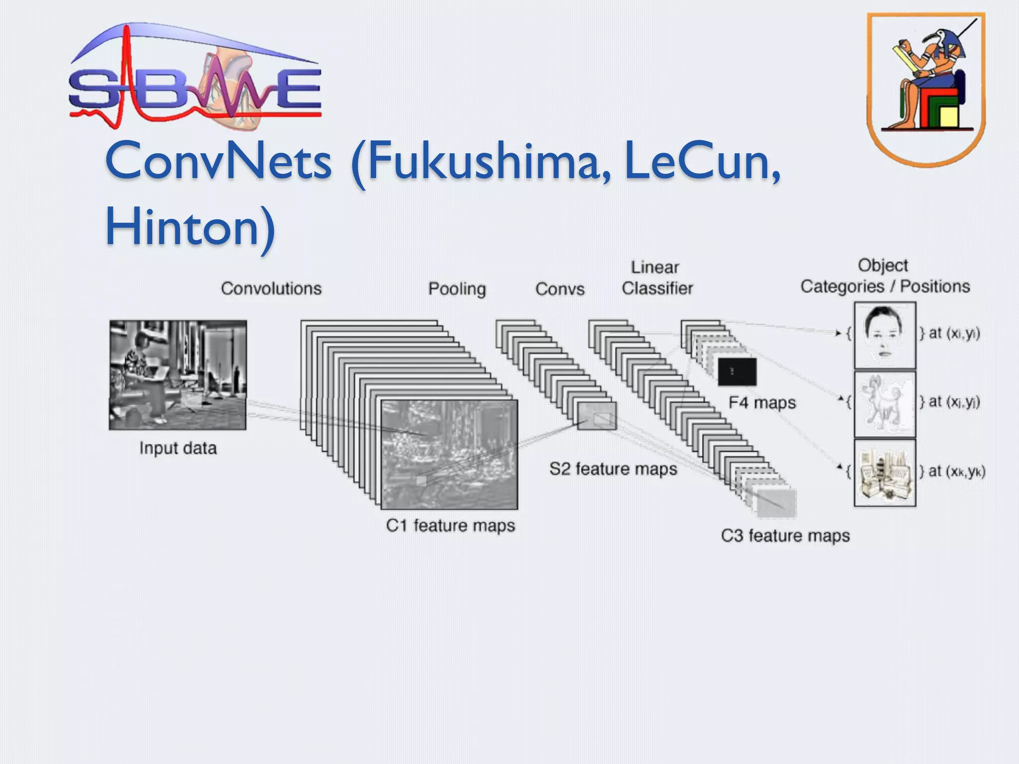
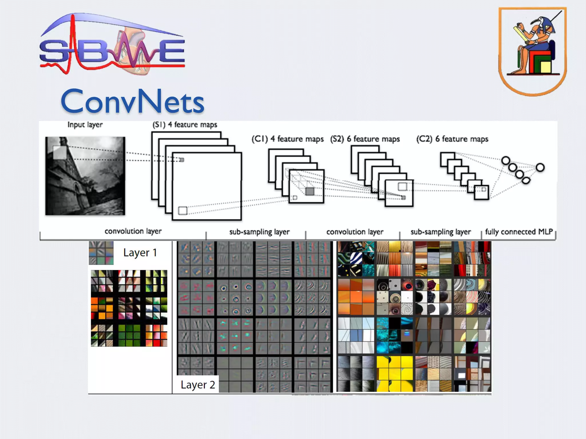
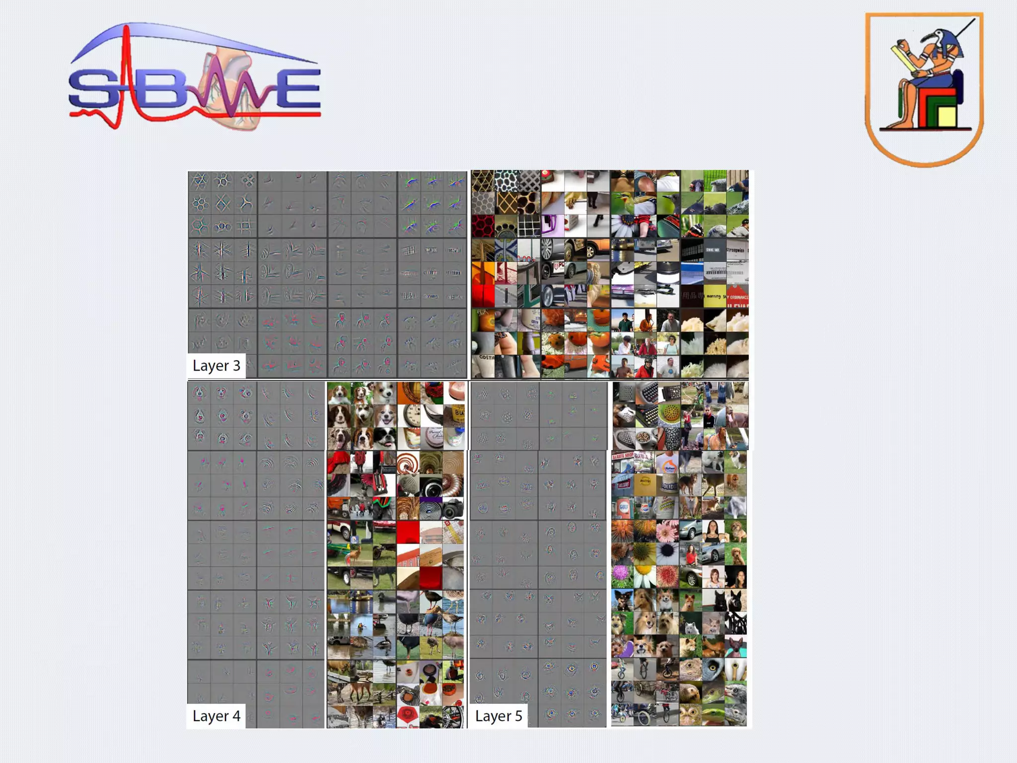
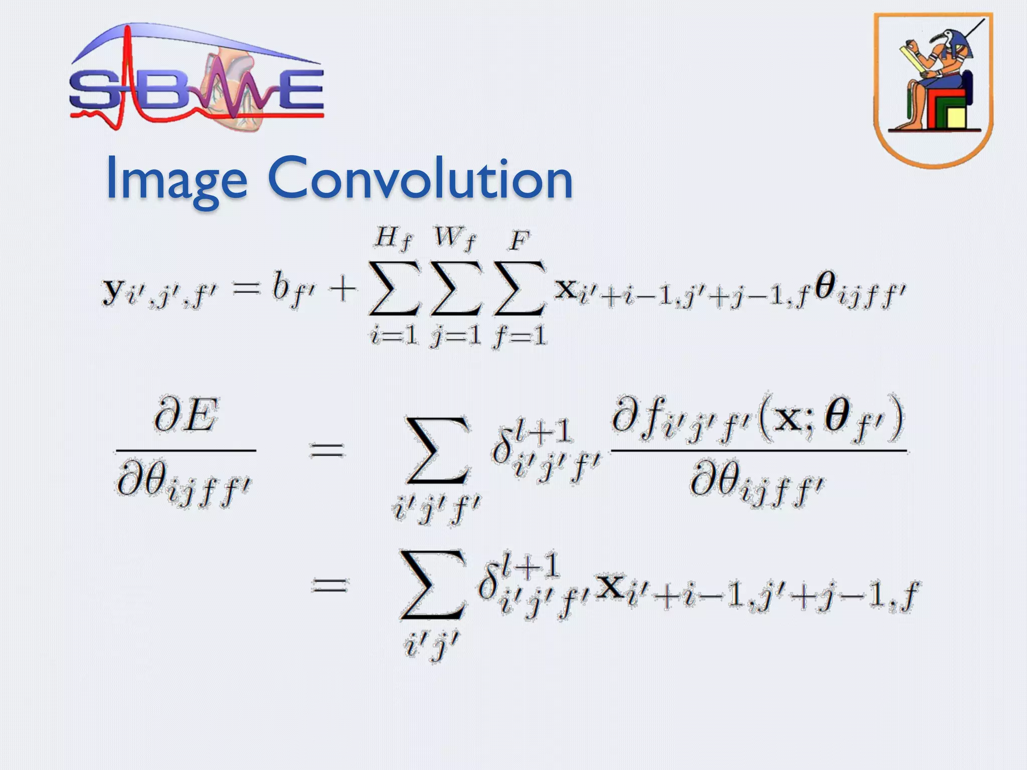
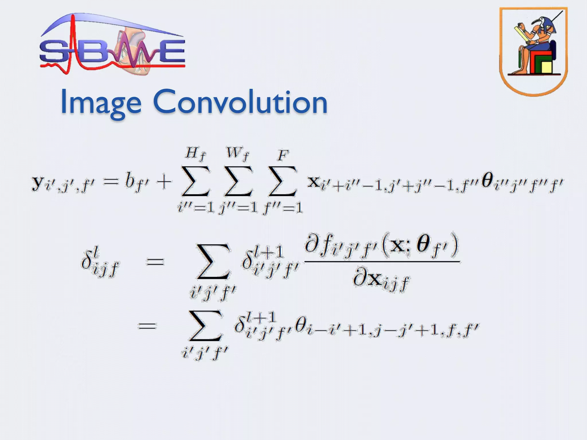
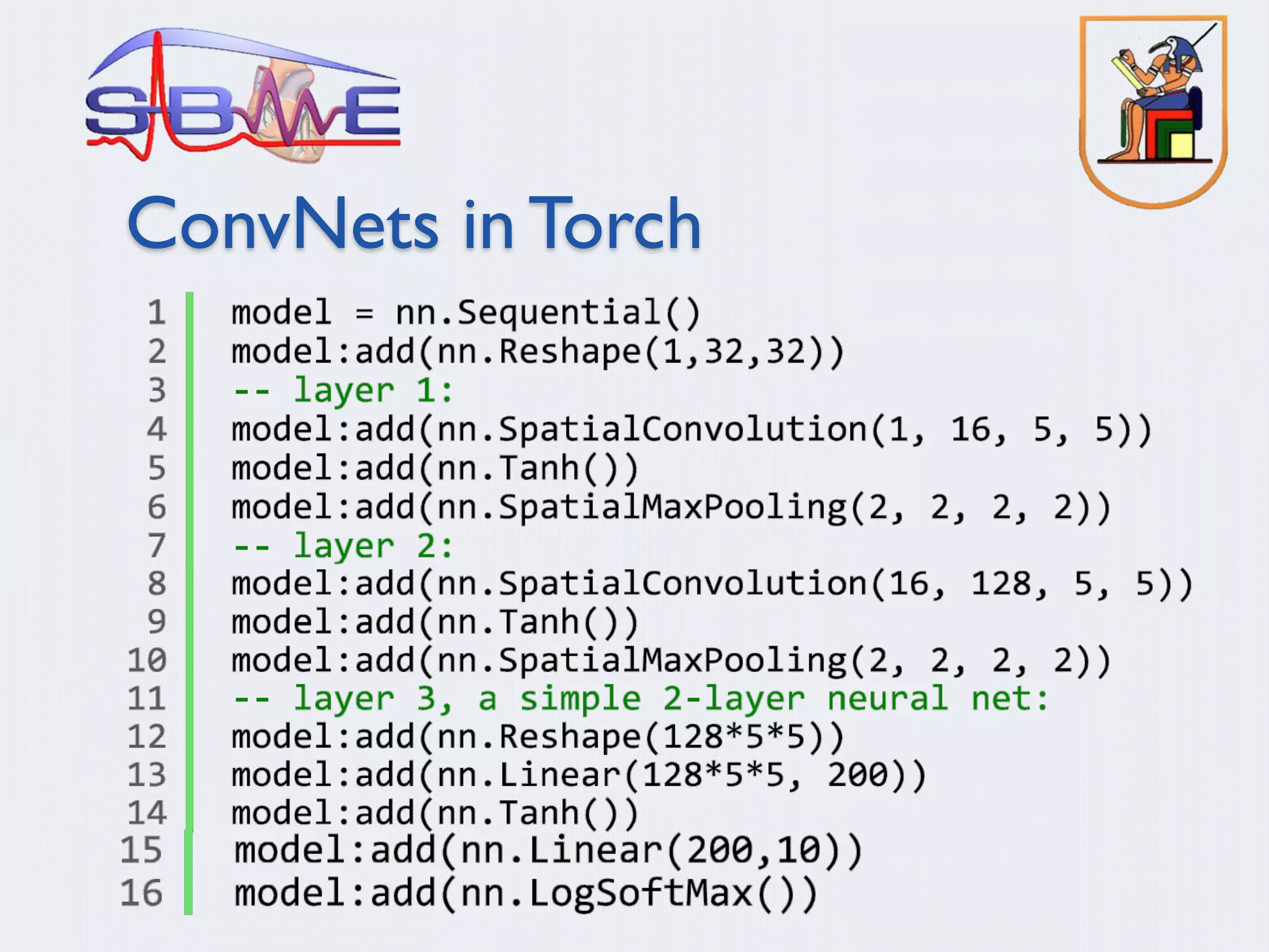
§ Deep Convolution Neural Networks
§ Residual Networks
§ Seams Networks
§ Self Learning Netowrks
[Other related work: LeCun, Lee,Yuille, Ng …]](https://image.slidesharecdn.com/sbmemlpresentation2b-200812164346/75/Machine-Learning-2-7-2048.jpg)
![Learning an image representation
Sparse coding (Olshausen & Field,1996)
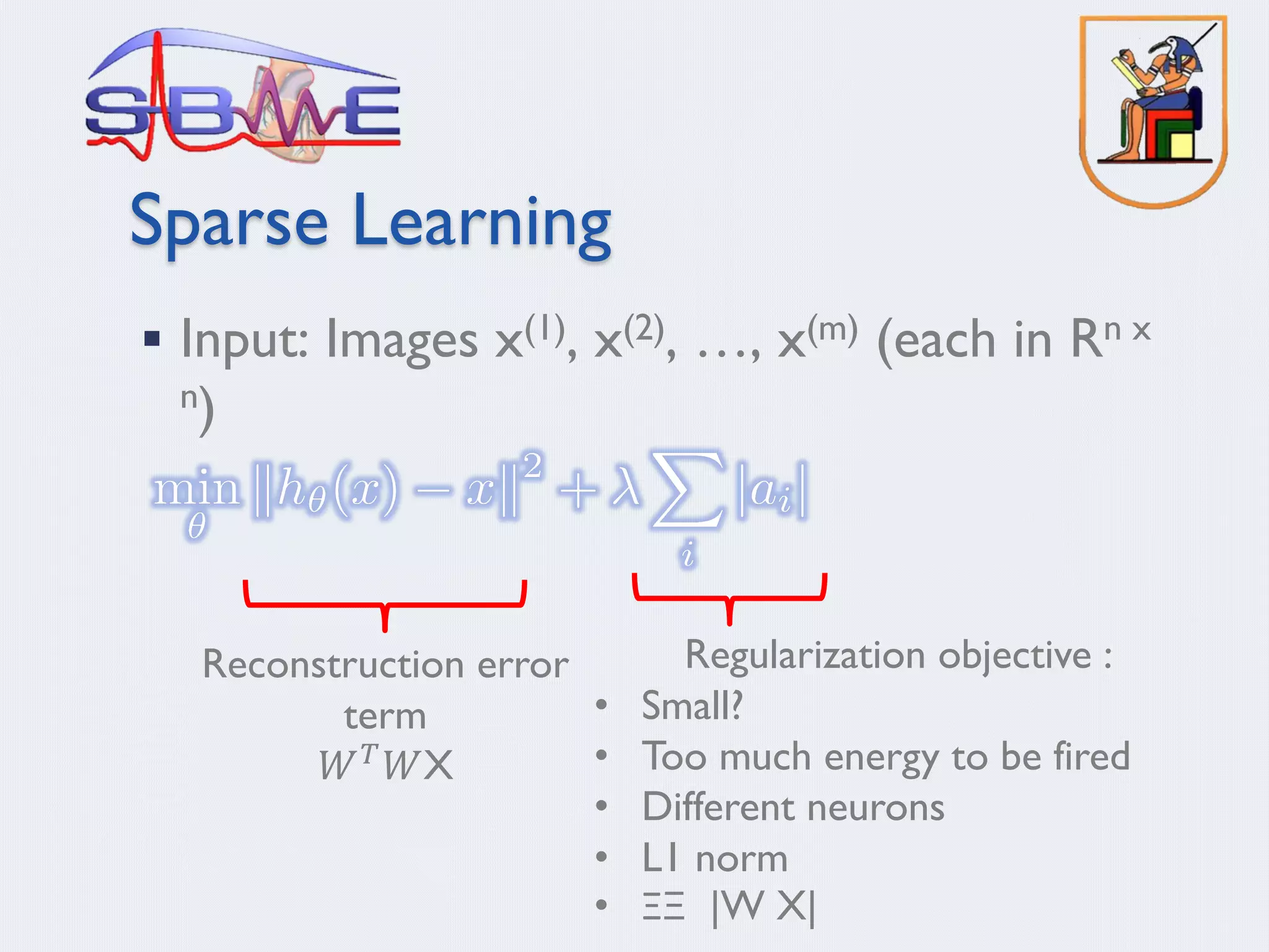
Input: Images x(1), x(2), …, x(m) (each in Rn x n)
Learn: Dictionary of bases f1, f2, …, fk (also Rn x n), so that each
input x can be approximately decomposed as:
s.t. aj’s are mostly zero (“sparse”)
Use to represent 14x14 image patch succinctly, as [a7=0.8, a36=0.3,
a41 = 0.5]. I.e., this indicates which “basic edges” make up the
image.](https://image.slidesharecdn.com/sbmemlpresentation2b-200812164346/75/Machine-Learning-2-22-2048.jpg)
![Sparse coding illustration
Natural Images
Learned bases (f1 , …, f64): “Edges”
50 100 150 200 250 300 350 400 450 500
50
100
150
200
250
300
350
400
450
500
50 100 150 200 250 300 350 400 450 500
50
100
150
200
250
300
350
400
450
500
50 100 150 200 250 300 350 400 450 500
50
100
150
200
250
300
350
400
450
500
» 0.8 * + 0.3 * + 0.5 *
x » 0.8 * f36
+ 0.3 * f42 + 0.5 * f63
[0, 0, …, 0, 0.8, 0, …, 0, 0.3, 0, …, 0, 0.5, …]
Test example](https://image.slidesharecdn.com/sbmemlpresentation2b-200812164346/75/Machine-Learning-2-23-2048.jpg)
![Represent as: [0, 0, …, 0, 0.6, 0, …, 0, 0.8, 0, …, 0, 0.4, …]
Represent as: [0, 0, …, 0, 1.3, 0, …, 0, 0.9, 0, …, 0, 0.3, …]
More examples
» 0.6 * + 0.8 * + 0.4 *
f15 f28
f37
» 1.3 * + 0.9 * + 0.3 *
f5 f18
f29
• Method hypothesizes that edge-like patches are the most
“basic” elements of a scene, and represents an image in terms of
the edges that appear in it.
• Use to obtain a more compact, higher-level representation of
the scene than pixels.](https://image.slidesharecdn.com/sbmemlpresentation2b-200812164346/75/Machine-Learning-2-24-2048.jpg)

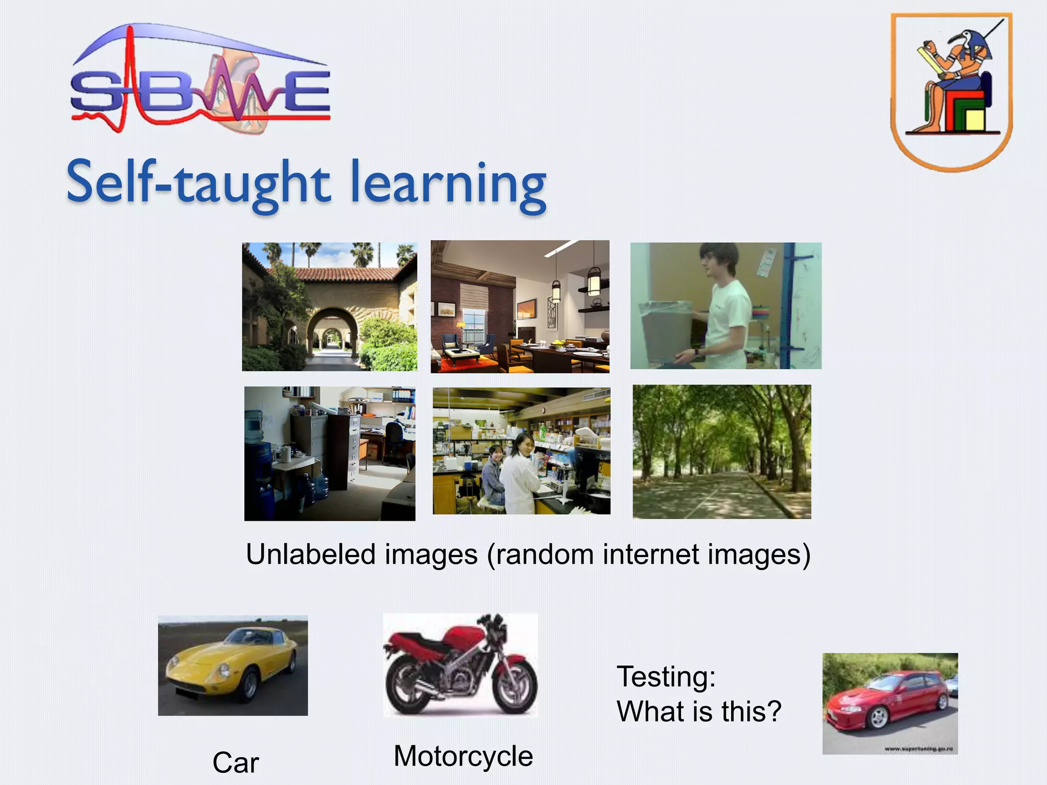
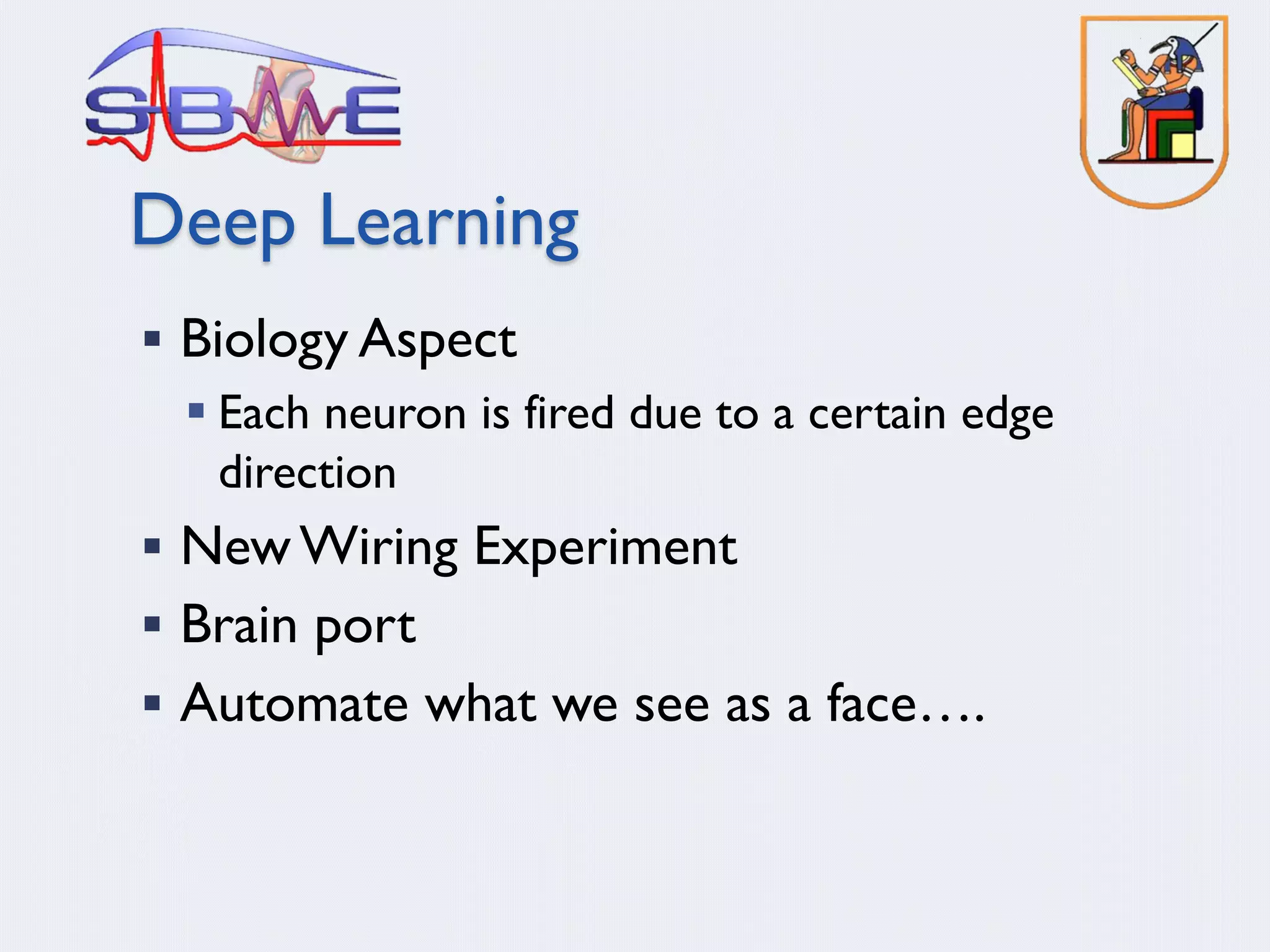
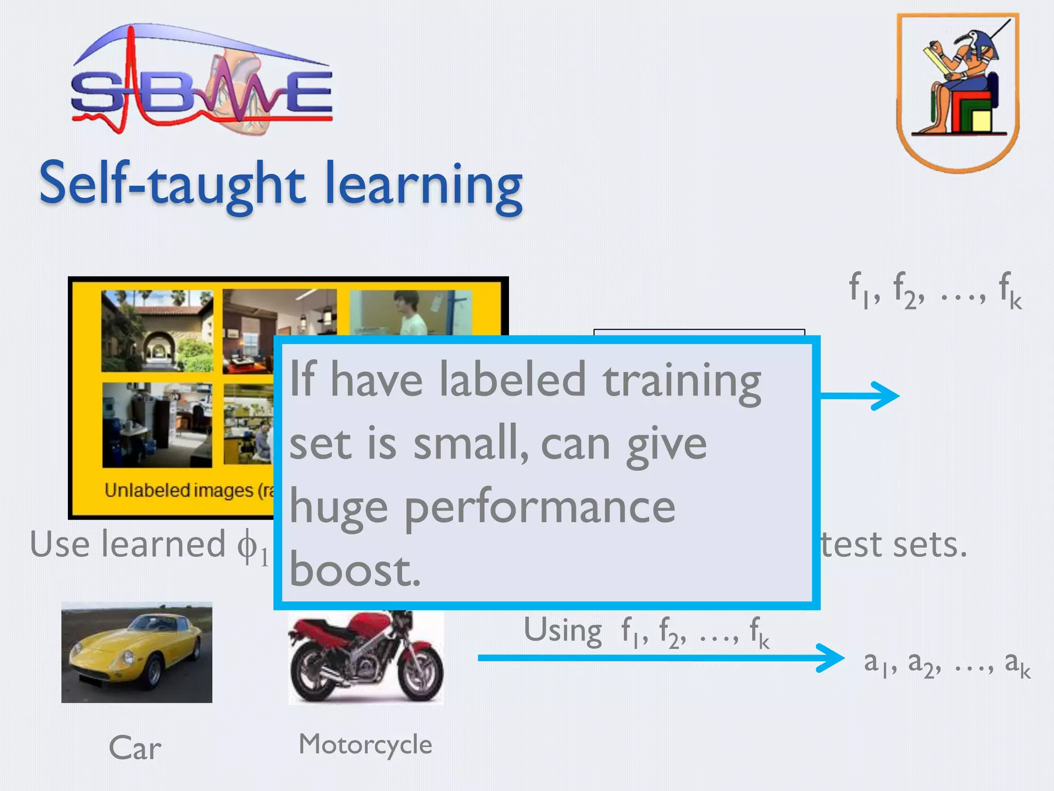
This document discusses machine learning and deep learning techniques. It begins with an overview of self-taught learning and testing unlabeled images. It then discusses biology aspects of neural networks and experiments with brain ports. The remainder of the document focuses on deep learning algorithms including deep belief networks, deep sparse autoencoders, deep convolution neural networks, and residual networks. It also discusses using autoencoders for unsupervised feature learning and greedy learning approaches. Finally, it provides an overview of convolution neural networks including their use in visual processing and image representation.