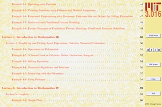
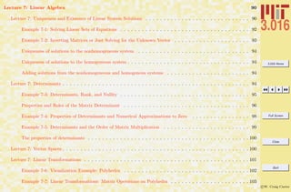
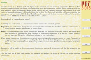
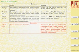
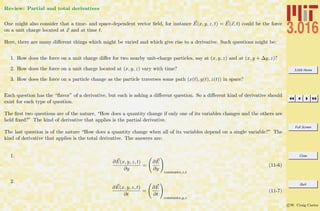
This document outlines the structure and expectations for the 3.016 course. It discusses the software used, Mathematica, examination and homework policies, grading, and the textbook and lecture materials. It also provides examples of common Mathematica commands and mistakes to avoid when getting started with the software.

1. 3.016 Home
Full Screen
Close
Quit
c W. Craig Carter
Contents
INDEX (Linked) 347
Lecture 1: Introduction and Course Description 2
Lecture 1: Preface . . . . . . . . . . . . . . . . . . . . . . . . . . . . . . . . . . . . . . . . . . . . . . . . . . . . . . . 2
Lecture 1: 3.016 Mathematical Software . . . . . . . . . . . . . . . . . . . . . . . . . . . . . . . . . . . . . . . . . . . 3
Lecture 1: 3.016 Examination Philosophy . . . . . . . . . . . . . . . . . . . . . . . . . . . . . . . . . . . . . . . . . . 4
Lecture 1: 3.016 Homework . . . . . . . . . . . . . . . . . . . . . . . . . . . . . . . . . . . . . . . . . . . . . . . . . . 5
Lecture 1: 3.016 Laboratory . . . . . . . . . . . . . . . . . . . . . . . . . . . . . . . . . . . . . . . . . . . . . . . . . . 7
Lecture 1: Grades . . . . . . . . . . . . . . . . . . . . . . . . . . . . . . . . . . . . . . . . . . . . . . . . . . . . . . . 8
Lecture 1: Homework Calendar and Weighting . . . . . . . . . . . . . . . . . . . . . . . . . . . . . . . . . . . . . . . 9
Lecture 1: Late Policy . . . . . . . . . . . . . . . . . . . . . . . . . . . . . . . . . . . . . . . . . . . . . . . . . . . . . 9
Lecture 1: Textbook . . . . . . . . . . . . . . . . . . . . . . . . . . . . . . . . . . . . . . . . . . . . . . . . . . . . . . 10
Lecture 1: Lecture Notes . . . . . . . . . . . . . . . . . . . . . . . . . . . . . . . . . . . . . . . . . . . . . . . . . . . 10
Lecture 1: Lecture and Laboratory Calendar . . . . . . . . . . . . . . . . . . . . . . . . . . . . . . . . . . . . . . . . 11
Lecture 1: Beginners to Mathematica . . . . . . . . . . . . . . . . . . . . . . . . . . . . . . . . . . . . . . . . . . . 25
Example 1-1: Common Mathematica Mistakes . . . . . . . . . . . . . . . . . . . . . . . . . . . . . . . . . . . . 26

2. 3.016 Home
Full Screen
Close
Quit
c W. Craig Carter
Example 1-2: Common Mathematica Mistakes . . . . . . . . . . . . . . . . . . . . . . . . . . . . . . . . . . . . 27
Example 1-3: Common Mathematica Mistakes . . . . . . . . . . . . . . . . . . . . . . . . . . . . . . . . . . . . 28
Lecture 2: Introduction to Mathematica 29
Lecture 2: Expressions and Evaluation . . . . . . . . . . . . . . . . . . . . . . . . . . . . . . . . . . . . . . . . . . . . 29
Getting Started . . . . . . . . . . . . . . . . . . . . . . . . . . . . . . . . . . . . . . . . . . . . . . . . . . . . . . 29
Example 2-1: Basic Input and Assignment . . . . . . . . . . . . . . . . . . . . . . . . . . . . . . . . . . . . . . . 31
Example 2-2: Building Expressions and Functions and Operations on Expressions . . . . . . . . . . . . . . . . . 32
Example 2-3: Calculus and Plotting . . . . . . . . . . . . . . . . . . . . . . . . . . . . . . . . . . . . . . . . . . 33
Example 2-4: Lists, Lists of Lists, and Operations on Lists . . . . . . . . . . . . . . . . . . . . . . . . . . . . . . 34
Example 2-5: Rules (→) and Replacement (/.); Getting Help . . . . . . . . . . . . . . . . . . . . . . . . . . . . 35
Getting Help on Mathematica . . . . . . . . . . . . . . . . . . . . . . . . . . . . . . . . . . . . . . . . . . . . . . 36
Lecture 3: Introduction to Mathematica II 37
Lecture 3: Functions and Rules . . . . . . . . . . . . . . . . . . . . . . . . . . . . . . . . . . . . . . . . . . . . . . . . 37
Example 3-1: Procedural Programming . . . . . . . . . . . . . . . . . . . . . . . . . . . . . . . . . . . . . . . . 39
Example 3-2: Plotting Lists of Data and Examples of Deeper Mathematica R Functionality . . . . . . . . . 40
Example 3-3: Making Variables Local and Using Switches to Control Procedures . . . . . . . . . . . . . . . . . 42

3. 3.016 Home
Full Screen
Close
Quit
c W. Craig Carter
Example 3-4: Operating with Patterns . . . . . . . . . . . . . . . . . . . . . . . . . . . . . . . . . . . . . . . . . 44
Example 3-5: Creating Functions using Patterns and Delayed Assignment . . . . . . . . . . . . . . . . . . . . . 45
Example 3-6: Functional Programming with Recursion: Functions that are Defined by Calling Themselves . . . 47
Example 3-7: Restricted and Conditional Pattern Matching . . . . . . . . . . . . . . . . . . . . . . . . . . . . . 48
Example 3-8: Further Examples of Conditional Pattern Matching; Conditional Function Definitions . . . . . . 49
Lecture 4: Introduction to Mathematica III 50
Lecture 4: Simplifying and Picking Apart Expressions, Calculus, Numerical Evaluation . . . . . . . . . . . . . . . . . 50
Example 4-1: Operations on Polynomials . . . . . . . . . . . . . . . . . . . . . . . . . . . . . . . . . . . . . . . 51
Example 4-2: A Second Look at Calculus: Limits, Derivatives, Integrals . . . . . . . . . . . . . . . . . . . . . . 52
Example 4-3: Solving Equations . . . . . . . . . . . . . . . . . . . . . . . . . . . . . . . . . . . . . . . . . . . . 53
Example 4-4: Numerical Algorithms and Solutions . . . . . . . . . . . . . . . . . . . . . . . . . . . . . . . . . . 55
Example 4-5: Interacting with the Filesystem . . . . . . . . . . . . . . . . . . . . . . . . . . . . . . . . . . . . . 57
Example 4-6: Using Packages . . . . . . . . . . . . . . . . . . . . . . . . . . . . . . . . . . . . . . . . . . . . . . 58
Lecture 5: Introduction to Mathematica IV 59
Lecture 5: Graphics . . . . . . . . . . . . . . . . . . . . . . . . . . . . . . . . . . . . . . . . . . . . . . . . . . . . . . 59
Example 5-1: Simple Plots . . . . . . . . . . . . . . . . . . . . . . . . . . . . . . . . . . . . . . . . . . . . . . . . 60

4. 3.016 Home
Full Screen
Close
Quit
c W. Craig Carter
Example 5-2: Plotting Precision and an Example of Interaction . . . . . . . . . . . . . . . . . . . . . . . . . . . 61
Example 5-3: Multiple Curves, Filling, and Excluding Points . . . . . . . . . . . . . . . . . . . . . . . . . . . . 62
Example 5-4: Plotting Two Dimensional Parametric Curves and Mapped Regions . . . . . . . . . . . . . . . . . 63
Example 5-5: Simple Plots of Data . . . . . . . . . . . . . . . . . . . . . . . . . . . . . . . . . . . . . . . . . . . 64
Example 5-6: Getting More out of Displayed Data: Screen Interaction . . . . . . . . . . . . . . . . . . . . . . . 65
Example 5-7: Graphical Data Exploration, continued . . . . . . . . . . . . . . . . . . . . . . . . . . . . . . . . . 66
Example 5-8: Three-Dimensional Graphics . . . . . . . . . . . . . . . . . . . . . . . . . . . . . . . . . . . . . . . 67
Example 5-9: Colors and Contours: Three-Dimensional Graphics in Two Dimensions . . . . . . . . . . . . . . . 68
Example 5-10: Graphics Primitives, Drawing on Graphics, and Combining Graphical Objects . . . . . . . . . . 69
Example 5-11: A Worked Example: The Two-Dimensional Wulff Construction . . . . . . . . . . . . . . . . . . 70
Lecture 5: Graphical Animation: Using Time as a Dimension in Visualization . . . . . . . . . . . . . . . . . . . . . . 71
Example 5-12: Animation . . . . . . . . . . . . . . . . . . . . . . . . . . . . . . . . . . . . . . . . . . . . . . . . 72
Example 5-13: An Example of Animating a Random Walk . . . . . . . . . . . . . . . . . . . . . . . . . . . . . . 73
Example 5-14: Worked Example (part A): Visualizing the Spinodal and Common Tangent Construction . . . . 74
Example 5-15: Worked Example (part B): Visualizing the Spinodal and Common Tangent Construction . . . . 75
Example 5-16: Worked Example (part C): Visualizing the Spinodal and Common Tangent Construction . . . . 76
Example 5-17: Worked Example (part D): Visualizing the Spinodal and Common Tangent Construction . . . . 77

5. 3.016 Home
Full Screen
Close
Quit
c W. Craig Carter
Example 5-18: Worked Example (part E): Visualizing the Spinodal and Common Tangent Construction . . . . 78
Lecture 6: Linear Algebra I 79
Lecture 6: Vectors . . . . . . . . . . . . . . . . . . . . . . . . . . . . . . . . . . . . . . . . . . . . . . . . . . . . . . . 79
Vectors as a list of associated information . . . . . . . . . . . . . . . . . . . . . . . . . . . . . . . . . . . . . . . 79
Scalar multiplication . . . . . . . . . . . . . . . . . . . . . . . . . . . . . . . . . . . . . . . . . . . . . . . . . . . 80
Vector norms . . . . . . . . . . . . . . . . . . . . . . . . . . . . . . . . . . . . . . . . . . . . . . . . . . . . . . . 81
Unit vectors . . . . . . . . . . . . . . . . . . . . . . . . . . . . . . . . . . . . . . . . . . . . . . . . . . . . . . . . 81
Lecture 6: Matrices and Matrix Operations . . . . . . . . . . . . . . . . . . . . . . . . . . . . . . . . . . . . . . . . . 81
Matrices as a linear transformation of a vector . . . . . . . . . . . . . . . . . . . . . . . . . . . . . . . . . . . . 82
Matrix transpose operations . . . . . . . . . . . . . . . . . . . . . . . . . . . . . . . . . . . . . . . . . . . . . . . 83
Matrix Multiplication . . . . . . . . . . . . . . . . . . . . . . . . . . . . . . . . . . . . . . . . . . . . . . . . . . 84
Example 6-1: Matrices . . . . . . . . . . . . . . . . . . . . . . . . . . . . . . . . . . . . . . . . . . . . . . . . . . 85
Matrix Inversion . . . . . . . . . . . . . . . . . . . . . . . . . . . . . . . . . . . . . . . . . . . . . . . . . . . . . 86
Example 6-2: Inverting Matrices . . . . . . . . . . . . . . . . . . . . . . . . . . . . . . . . . . . . . . . . . . . . 87
Linear Independence: When solutions exist . . . . . . . . . . . . . . . . . . . . . . . . . . . . . . . . . . . . . . 88
Example 6-3: Eliminating redundant equations or variables . . . . . . . . . . . . . . . . . . . . . . . . . . . . . 89

6. 3.016 Home
Full Screen
Close
Quit
c W. Craig Carter
Lecture 7: Linear Algebra 90
Lecture 7: Uniqueness and Existence of Linear System Solutions . . . . . . . . . . . . . . . . . . . . . . . . . . . . . 90
Example 7-1: Solving Linear Sets of Equations . . . . . . . . . . . . . . . . . . . . . . . . . . . . . . . . . . . . 92
Example 7-2: Inverting Matrices or Just Solving for the Unknown Vector . . . . . . . . . . . . . . . . . . . . . 93
Uniqueness of solutions to the nonhomogeneous system . . . . . . . . . . . . . . . . . . . . . . . . . . . . . . . 94
Uniqueness of solutions to the homogeneous system . . . . . . . . . . . . . . . . . . . . . . . . . . . . . . . . . . 94
Adding solutions from the nonhomogeneous and homogenous systems . . . . . . . . . . . . . . . . . . . . . . . 94
Lecture 7: Determinants . . . . . . . . . . . . . . . . . . . . . . . . . . . . . . . . . . . . . . . . . . . . . . . . . . . . 94
Example 7-3: Determinants, Rank, and Nullity . . . . . . . . . . . . . . . . . . . . . . . . . . . . . . . . . . . . 95
Properties and Roles of the Matrix Determinant . . . . . . . . . . . . . . . . . . . . . . . . . . . . . . . . . . . 96
Example 7-4: Properties of Determinants and Numerical Approximations to Zero . . . . . . . . . . . . . . . . 98
Example 7-5: Determinants and the Order of Matrix Multiplication . . . . . . . . . . . . . . . . . . . . . . . . 99
The properties of determinants . . . . . . . . . . . . . . . . . . . . . . . . . . . . . . . . . . . . . . . . . . . . . 100
Lecture 7: Vector Spaces . . . . . . . . . . . . . . . . . . . . . . . . . . . . . . . . . . . . . . . . . . . . . . . . . . . . 100
Lecture 7: Linear Transformations . . . . . . . . . . . . . . . . . . . . . . . . . . . . . . . . . . . . . . . . . . . . . . 101
Example 7-6: Visualization Example: Polyhedra . . . . . . . . . . . . . . . . . . . . . . . . . . . . . . . . . . . 102
Example 7-7: Linear Transformations: Matrix Operations on Polyhedra . . . . . . . . . . . . . . . . . . . . . . 103

7. 3.016 Home
Full Screen
Close
Quit
c W. Craig Carter
Example 7-8: Visualization Example: Invariant Symmetry Operations on Crystals . . . . . . . . . . . . . . . . 104
Lecture 8: Complex Numbers and Euler’s Formula 105
Lecture 8: Complex Numbers and Operations in the Complex Plane . . . . . . . . . . . . . . . . . . . . . . . . . . . 105
Example 8-1: Operations on complex numbers . . . . . . . . . . . . . . . . . . . . . . . . . . . . . . . . . . . . 107
Complex Plane and Complex Conjugates . . . . . . . . . . . . . . . . . . . . . . . . . . . . . . . . . . . . . . . 108
Lecture 8: Polar Form of Complex Numbers . . . . . . . . . . . . . . . . . . . . . . . . . . . . . . . . . . . . . . . . . 109
Multiplication, Division, and Roots in Polar Form . . . . . . . . . . . . . . . . . . . . . . . . . . . . . . . . . . 109
Example 8-2: Numerical Properties of Operations on Complex Numbers . . . . . . . . . . . . . . . . . . . . . . 110
Lecture 8: Exponentiation and Relations to Trignometric Functions . . . . . . . . . . . . . . . . . . . . . . . . . . . 111
Lecture 8: Complex Numbers in Roots to Polynomial Equations . . . . . . . . . . . . . . . . . . . . . . . . . . . . . 111
Example 8-3: Complex Roots of Polynomial Equations . . . . . . . . . . . . . . . . . . . . . . . . . . . . . . . . 112
Lecture 9: Eigensystems of Matrix Equations 113
Lecture 9: Eigenvalues and Eigenvectors of a Matrix . . . . . . . . . . . . . . . . . . . . . . . . . . . . . . . . . . . . 113
Example 9-1: Calculating Matrix Eigenvalues and Eigenvectors . . . . . . . . . . . . . . . . . . . . . . . . . . . 115
Lecture 9: Symmetric, Skew-Symmetric, Orthogonal Matrices . . . . . . . . . . . . . . . . . . . . . . . . . . . . . . . 119
Orthogonal Transformations . . . . . . . . . . . . . . . . . . . . . . . . . . . . . . . . . . . . . . . . . . . . . . . 121

8. 3.016 Home
Full Screen
Close
Quit
c W. Craig Carter
Example 9-2: Coordinate Transformations to The Eigenbasis . . . . . . . . . . . . . . . . . . . . . . . . . . . . 123
Lecture 10: Real Eigenvalue Systems; Transformations to Eigenbasis 124
Lecture 10: Similarity Transformations . . . . . . . . . . . . . . . . . . . . . . . . . . . . . . . . . . . . . . . . . . . . 124
Stresses and Strains . . . . . . . . . . . . . . . . . . . . . . . . . . . . . . . . . . . . . . . . . . . . . . . . . . . 127
EigenStrains and EigenStresses . . . . . . . . . . . . . . . . . . . . . . . . . . . . . . . . . . . . . . . . . . . . . 130
Example 10-1: Representations of Stress (or Strain) in Rotated Coordinate Systems . . . . . . . . . . . . . . . 131
Example 10-2: Principal Axes: Mohr’s Circle of Two-Dimensional Stress . . . . . . . . . . . . . . . . . . . . . . 132
Example 10-3: Visualization Example: Graphics for Mohr’s Circle . . . . . . . . . . . . . . . . . . . . . . . . . 134
Example 10-4: Interactive Graphics Demonstration for Mohr’s Circle . . . . . . . . . . . . . . . . . . . . . . . . 135
Lecture 10: Quadratic Forms . . . . . . . . . . . . . . . . . . . . . . . . . . . . . . . . . . . . . . . . . . . . . . . . . 136
Lecture 10: Eigenvector Basis . . . . . . . . . . . . . . . . . . . . . . . . . . . . . . . . . . . . . . . . . . . . . . . . . 137
Lecture 11: Geometry and Calculus of Vectors 139
Lecture 11: Vector Products . . . . . . . . . . . . . . . . . . . . . . . . . . . . . . . . . . . . . . . . . . . . . . . . . . 139
Review: The Inner (dot) product of two vectors and relation to projection . . . . . . . . . . . . . . . . . . . . . 140
Review: Vector (or cross-) products . . . . . . . . . . . . . . . . . . . . . . . . . . . . . . . . . . . . . . . . . . 141
Example 11-1: Cross Product Example . . . . . . . . . . . . . . . . . . . . . . . . . . . . . . . . . . . . . . . . . 143

9. 3.016 Home
Full Screen
Close
Quit
c W. Craig Carter
Example 11-2: Visualizing Space-Curves as Time-Dependent Vectors . . . . . . . . . . . . . . . . . . . . . . . . 144
Lecture 11: Derivatives of Vectors . . . . . . . . . . . . . . . . . . . . . . . . . . . . . . . . . . . . . . . . . . . . . . 145
Example 11-3: Visualizing Time-Dependent Vectors and their Derivatives . . . . . . . . . . . . . . . . . . . . . 146
Review: Partial and total derivatives . . . . . . . . . . . . . . . . . . . . . . . . . . . . . . . . . . . . . . . . . . 147
Lecture 11: Time-Dependent Scalar and Vector Fields . . . . . . . . . . . . . . . . . . . . . . . . . . . . . . . . . . . 148
Example 11-4: Visualizing a Solution to the Diffusion Equation . . . . . . . . . . . . . . . . . . . . . . . . . . . 149
Example 11-5: Visualizing the Diffusion Flux: The Time-Dependent Gradient Field . . . . . . . . . . . . . . . 150
All vectors are not spatial . . . . . . . . . . . . . . . . . . . . . . . . . . . . . . . . . . . . . . . . . . . . . . . . 151
Lecture 12: Multivariable Calculus 152
Lecture 12: The Calculus of Curves . . . . . . . . . . . . . . . . . . . . . . . . . . . . . . . . . . . . . . . . . . . . . 152
Example 12-1: Embedding Curves in Surfaces in Three Dimensions . . . . . . . . . . . . . . . . . . . . . . . . . 154
Using Arc-Length as a Curve’s Parameter . . . . . . . . . . . . . . . . . . . . . . . . . . . . . . . . . . . . . . . 156
Example 12-2: Calculating arclength . . . . . . . . . . . . . . . . . . . . . . . . . . . . . . . . . . . . . . . . . . 157
Lecture 12: Scalar Functions with Vector Argument . . . . . . . . . . . . . . . . . . . . . . . . . . . . . . . . . . . . 158
How Confusion Can Develop in Thermodynamics . . . . . . . . . . . . . . . . . . . . . . . . . . . . . . . . . . . 159
Lecture 12: Total and Partial Derivatives, Chain Rule . . . . . . . . . . . . . . . . . . . . . . . . . . . . . . . . . . . 160
Example 12-3: Total Derivatives and Partial Derivatives: A Mathematica Review . . . . . . . . . . . . . . . . . 161

10. 3.016 Home
Full Screen
Close
Quit
c W. Craig Carter
Taylor Series . . . . . . . . . . . . . . . . . . . . . . . . . . . . . . . . . . . . . . . . . . . . . . . . . . . . . . . 162
Example 12-4: Taylor Expansions of a Scalar Function of v in the Neighborhood of Zero . . . . . . . . . . . . . 164
Example 12-5: Approximating Surfaces at Points . . . . . . . . . . . . . . . . . . . . . . . . . . . . . . . . . . . 165
Lecture 12: Gradients and Directional Derivatives . . . . . . . . . . . . . . . . . . . . . . . . . . . . . . . . . . . . . 168
Finding the Gradient . . . . . . . . . . . . . . . . . . . . . . . . . . . . . . . . . . . . . . . . . . . . . . . . . . . 169
Potentials and Force Fields . . . . . . . . . . . . . . . . . . . . . . . . . . . . . . . . . . . . . . . . . . . . . . . 169
Lecture 13: Differential Operations on Vectors 171
Lecture 13: Generalizing the Derivative . . . . . . . . . . . . . . . . . . . . . . . . . . . . . . . . . . . . . . . . . . . 171
Example 13-1: Scalar Potentials and their Gradient Fields . . . . . . . . . . . . . . . . . . . . . . . . . . . . . 173
Lecture 13: Divergence and Its Interpretation . . . . . . . . . . . . . . . . . . . . . . . . . . . . . . . . . . . . . . . . 174
Example 13-2: Visualizing the Gradient Field and its Divergence: The Laplacian . . . . . . . . . . . . . . . . . 175
Coordinate Systems . . . . . . . . . . . . . . . . . . . . . . . . . . . . . . . . . . . . . . . . . . . . . . . . . . . 176
Example 13-3: Coordinate Transformations . . . . . . . . . . . . . . . . . . . . . . . . . . . . . . . . . . . . . . 177
Example 13-4: Frivolous Example Using Geodesy, VectorAnalysis, and CityData. . . . . . . . . . . . . . . . 178
Example 13-5: Gradient and Divergence Operations in Other Coordinate Systems . . . . . . . . . . . . . . . . 179
Lecture 13: Curl and Its Interpretation . . . . . . . . . . . . . . . . . . . . . . . . . . . . . . . . . . . . . . . . . . . 180
Example 13-6: Computing and Visualizing Curl Fields . . . . . . . . . . . . . . . . . . . . . . . . . . . . . . . . 181

11. 3.016 Home
Full Screen
Close
Quit
c W. Craig Carter
Lecture 14: Integrals along a Path 184
Lecture 14: Integrals along a Curve . . . . . . . . . . . . . . . . . . . . . . . . . . . . . . . . . . . . . . . . . . . . . . 184
Path-Independence and Path-Integration . . . . . . . . . . . . . . . . . . . . . . . . . . . . . . . . . . . . . . . . 185
Example 14-1: Path Dependence of Integration of Vector Function: Non-Vanishing Curl . . . . . . . . . . . . . 186
Example 14-2: Examples of Path-Independence of Curl-Free Vector Fields . . . . . . . . . . . . . . . . . . . . . 187
Example 14-3: Examples of Path-Independence of Curl-Free Vector Fields on a Restricted Subspace . . . . . . 188
Lecture 14: Multidimensional Integrals . . . . . . . . . . . . . . . . . . . . . . . . . . . . . . . . . . . . . . . . . . . . 189
Lecture 14: Using Jacobians to Change Variables in Thermodynamic Calculations . . . . . . . . . . . . . . . . . . . 190
14-0.0.1Example of a Multiple Integral: Electrostatic Potential above a Charged Region . . . . . . . . . . . . . 192
Example 14-4: Integrals over Variable Domains . . . . . . . . . . . . . . . . . . . . . . . . . . . . . . . . . . . . 193
Example 14-5: Potential near a Charged and Shaped Surface Patch: Brute Force . . . . . . . . . . . . . . . . . 194
Lecture 15: Surface Integrals and Some Related Theorems 195
Lecture 15: Green’s Theorem for Area in Plane Relating to its Bounding Curve . . . . . . . . . . . . . . . . . . . . . 195
Example 15-1: Converting an area-integral over a variable domain into a path-integral over its boundary . . . . 199
Example 15-2: Faster and More Accurate Numerical Integration by Using Green’s Theorem. . . . . . . . . . . . 200
Lecture 15: Representations of Surfaces . . . . . . . . . . . . . . . . . . . . . . . . . . . . . . . . . . . . . . . . . . . 201
Example 15-3: Representations of Surfaces: Graphs z = f(x, y) (part 1) . . . . . . . . . . . . . . . . . . . . . . 206

12. 3.016 Home
Full Screen
Close
Quit
c W. Craig Carter
Example 15-4: Representations of Surfaces: Graphs z = f(x, y) (part 2) . . . . . . . . . . . . . . . . . . . . . . 207
Example 15-5: A Frivolous Example for Graphs z = f(x, y): Floating Pixels from Images in 3D . . . . . . . . . 208
Example 15-6: A Frivolous Example for Graphs z = f(x, y): Creating and Animating Surfaces from Image
Sequences . . . . . . . . . . . . . . . . . . . . . . . . . . . . . . . . . . . . . . . . . . . . . . . . . . . . . 209
Example 15-7: Representations of Surfaces: Parametric Surfaces x(u, v) . . . . . . . . . . . . . . . . . . . . . . 210
Example 15-8: Representations of Surfaces: Level Sets constant = f(x, y, z) . . . . . . . . . . . . . . . . . . . . 211
Lecture 15: Integration over Surfaces . . . . . . . . . . . . . . . . . . . . . . . . . . . . . . . . . . . . . . . . . . . . . 212
Example 15-9: Example of an Integral over a Parametric Surface . . . . . . . . . . . . . . . . . . . . . . . . . . 213
Lecture 16: Integral Theorems 214
Lecture 16: Higher-dimensional Integrals . . . . . . . . . . . . . . . . . . . . . . . . . . . . . . . . . . . . . . . . . . . 214
Lecture 16: The Divergence Theorem . . . . . . . . . . . . . . . . . . . . . . . . . . . . . . . . . . . . . . . . . . . . 215
Example 16-1: London Dispersion Potential due to a Finite Body . . . . . . . . . . . . . . . . . . . . . . . . . . 219
Example 16-2: Cylinder Surface and Integrands . . . . . . . . . . . . . . . . . . . . . . . . . . . . . . . . . . . . 220
Example 16-3: Integrating over the Cylinder Surface . . . . . . . . . . . . . . . . . . . . . . . . . . . . . . . . . 221
Example 16-4: Integrating over the Cylinder’s Top Surface . . . . . . . . . . . . . . . . . . . . . . . . . . . . . . 222
Example 16-5: Integrating over the Cylinder’s Bottom Surface . . . . . . . . . . . . . . . . . . . . . . . . . . . 223
Efficiency and Speed Issues: When to Evaluate the Right-Hand-Side of a Function in Mathematica R . . . . 224

13. 3.016 Home
Full Screen
Close
Quit
c W. Craig Carter
Example 16-6: To Evaluate or Not to Evaluate when Defining Functions . . . . . . . . . . . . . . . . . . . . . . 225
Example 16-7: Visualizing the Hamaker Potential of a Finite Cylinder: Contours of Constant Potential . . . . 226
Example 16-8: Visualizing the Hamaker Potential of a Finite Cylinder: Three-Dimensional Plots . . . . . . . . 227
Lecture 16: Stokes’ Theorem . . . . . . . . . . . . . . . . . . . . . . . . . . . . . . . . . . . . . . . . . . . . . . . . . 228
Lecture 16: Maxwell’s equations . . . . . . . . . . . . . . . . . . . . . . . . . . . . . . . . . . . . . . . . . . . . . . . 228
Lecture 16: Ampere’s Law . . . . . . . . . . . . . . . . . . . . . . . . . . . . . . . . . . . . . . . . . . . . . . . . . . . 229
Lecture 16: Gauss’ Law . . . . . . . . . . . . . . . . . . . . . . . . . . . . . . . . . . . . . . . . . . . . . . . . . . . . 229
Lecture 17: Function Representation by Fourier Series 230
Lecture 17: Periodic Functions . . . . . . . . . . . . . . . . . . . . . . . . . . . . . . . . . . . . . . . . . . . . . . . . 230
Example 17-1: Playing with Audible Periodic Phenomena . . . . . . . . . . . . . . . . . . . . . . . . . . . . . . 231
Example 17-2: Music and Instruments . . . . . . . . . . . . . . . . . . . . . . . . . . . . . . . . . . . . . . . . . 232
Example 17-3: Random Notes and Instruments . . . . . . . . . . . . . . . . . . . . . . . . . . . . . . . . . . . . 233
Example 17-4: Using Mod to Create Periodic Functions . . . . . . . . . . . . . . . . . . . . . . . . . . . . . . . . 235
Lecture 17: Odd and Even Functions . . . . . . . . . . . . . . . . . . . . . . . . . . . . . . . . . . . . . . . . . . . . . 236
Lecture 17: Representing a particular function with a sum of other functions . . . . . . . . . . . . . . . . . . . . . . 236
Lecture 17: Fourier Series . . . . . . . . . . . . . . . . . . . . . . . . . . . . . . . . . . . . . . . . . . . . . . . . . . . 237
Example 17-5: Orthogonality of Trigonometric Functions . . . . . . . . . . . . . . . . . . . . . . . . . . . . . . 239

14. 3.016 Home
Full Screen
Close
Quit
c W. Craig Carter
Lecture 17: Other forms of the Fourier coefficients . . . . . . . . . . . . . . . . . . . . . . . . . . . . . . . . . . . . . 240
Example 17-6: Calculating Fourier Series Amplitudes . . . . . . . . . . . . . . . . . . . . . . . . . . . . . . . . . 242
Example 17-7: Approximations to Functions with Truncated Fourier Series . . . . . . . . . . . . . . . . . . . . 243
Example 17-8: Demonstration the used of functions defined in the FourierSeries-package . . . . . . . . . . . 244
Example 17-9: Recursive Calculation of a Truncated Fourier Series . . . . . . . . . . . . . . . . . . . . . . . . . 245
Example 17-10: Visualizing Convergence of the Fourier Series: Gibbs Phenomenon . . . . . . . . . . . . . . . . 246
Lecture 17: Complex Form of the Fourier Series . . . . . . . . . . . . . . . . . . . . . . . . . . . . . . . . . . . . . . . 247
Lecture 18: The Fourier Transform and its Interpretations 248
Lecture 18: Fourier Transforms . . . . . . . . . . . . . . . . . . . . . . . . . . . . . . . . . . . . . . . . . . . . . . . . 248
Higher Dimensional Fourier Transforms . . . . . . . . . . . . . . . . . . . . . . . . . . . . . . . . . . . . . . . . 250
Lecture 18: Properties of Fourier Transforms . . . . . . . . . . . . . . . . . . . . . . . . . . . . . . . . . . . . . . . . 251
Dirac Delta Functions . . . . . . . . . . . . . . . . . . . . . . . . . . . . . . . . . . . . . . . . . . . . . . . . . . 251
Parseval’s Theorem . . . . . . . . . . . . . . . . . . . . . . . . . . . . . . . . . . . . . . . . . . . . . . . . . . . . 252
Convolution Theorem . . . . . . . . . . . . . . . . . . . . . . . . . . . . . . . . . . . . . . . . . . . . . . . . . . 252
Example 18-1: Creating Images of Lattices for Subsequent Fourier Transform . . . . . . . . . . . . . . . . . . . 254
Example 18-2: Improving Visualization Contrast with ColorFunction . . . . . . . . . . . . . . . . . . . . . . . 255
Example 18-3: ImagePlot . . . . . . . . . . . . . . . . . . . . . . . . . . . . . . . . . . . . . . . . . . . . . . . . 256

15. 3.016 Home
Full Screen
Close
Quit
c W. Craig Carter
Discrete Fourier Transforms . . . . . . . . . . . . . . . . . . . . . . . . . . . . . . . . . . . . . . . . . . . . . . . 257
Example 18-4: Discrete Fourier Transforms on Simulated Lattices . . . . . . . . . . . . . . . . . . . . . . . . . . 258
Example 18-5: Simulating Diffraction Patterns . . . . . . . . . . . . . . . . . . . . . . . . . . . . . . . . . . . . 259
Example 18-6: Alternative Representations of Diffraction Data . . . . . . . . . . . . . . . . . . . . . . . . . . . 260
Example 18-7: Diffraction Patterns of Defective Lattices . . . . . . . . . . . . . . . . . . . . . . . . . . . . . . . 261
Example 18-8: Diffraction Patterns from Lattices with Thermal ‘Noise’ . . . . . . . . . . . . . . . . . . . . . . . 262
Example 18-9: Computational Microscopy . . . . . . . . . . . . . . . . . . . . . . . . . . . . . . . . . . . . . . . 263
Example 18-10: Visualizing Simulated Selected Area Diffraction . . . . . . . . . . . . . . . . . . . . . . . . . . 264
Example 18-11: Simulated Diffraction Imaging on a Polycrystal . . . . . . . . . . . . . . . . . . . . . . . . . . . 265
Example 18-12: Bright-Field and Dark-Field Imaging of a Lattice with Thermal Noise . . . . . . . . . . . . . . 266
Example 18-13: Selected Area Diffraction on Image Data . . . . . . . . . . . . . . . . . . . . . . . . . . . . . . 267
Lecture 19: Ordinary Differential Equations: Introduction 268
Lecture 19: Differential Equations: Introduction . . . . . . . . . . . . . . . . . . . . . . . . . . . . . . . . . . . . . . 268
Iterative Application of Function . . . . . . . . . . . . . . . . . . . . . . . . . . . . . . . . . . . . . . . . . . . . 269
Example 19-1: Iteration: First-Order Sequences from a Fixed Boundary Condition . . . . . . . . . . . . . . . . 270
Example 19-2: Iteration: First-Order Sequences with a Generalized Boundary Condition . . . . . . . . . . . . . 271
Example 19-3: Space-Covering Sequences: Families of Trajectories . . . . . . . . . . . . . . . . . . . . . . . . . 272

16. 3.016 Home
Full Screen
Close
Quit
c W. Craig Carter
Forward Differencing Methods: Explicit Methods . . . . . . . . . . . . . . . . . . . . . . . . . . . . . . . . . . . 273
Example 19-4: First-Order Finite Differences: Method 1 Explicit Finite Differences . . . . . . . . . . . . . . . . 274
Example 19-5: Visualizing Trajectories from Explicit Forward Differences . . . . . . . . . . . . . . . . . . . . . 275
Forward Differencing Methods: Implicit Methods . . . . . . . . . . . . . . . . . . . . . . . . . . . . . . . . . . . 276
Example 19-6: First-Order Finite Differences: Method 1 Explicit Finite Differences . . . . . . . . . . . . . . . . 277
Example 19-7: Comparison of Implicit and Explicit Methods . . . . . . . . . . . . . . . . . . . . . . . . . . . . 278
Lecture 19: Geometrical Interpretation of Solutions . . . . . . . . . . . . . . . . . . . . . . . . . . . . . . . . . . . . . 279
Example 19-8: Visual Understanding of the Behavior of First-Order ODES . . . . . . . . . . . . . . . . . . . . 280
Example 19-9: Visualizing the Geometry of Flows for First-Order ODES . . . . . . . . . . . . . . . . . . . . . . 281
Example 19-10: Visualizing the Geometry of Flows for First-Order ODES . . . . . . . . . . . . . . . . . . . . . 282
Lecture 19: Separable Equations . . . . . . . . . . . . . . . . . . . . . . . . . . . . . . . . . . . . . . . . . . . . . . . 283
Example 19-11: Using Mathematica R ’s Built-in Ordinary Differential Equation Solver . . . . . . . . . . . . 284
Example 19-12: Comparision of Exact Solutions to Finite Difference Methods . . . . . . . . . . . . . . . . . . . 285
Example 19-13: Using Mathematica R ’s Differential Equation Solver on a First-Order ODE: Less Trivial
Example . . . . . . . . . . . . . . . . . . . . . . . . . . . . . . . . . . . . . . . . . . . . . . . . . . . . . . 287
Lecture 20: Linear Homogeneous and Heterogeneous ODEs 288
Lecture 20: Ordinary Differential Equations from Physical Models . . . . . . . . . . . . . . . . . . . . . . . . . . . . 288

17. 3.016 Home
Full Screen
Close
Quit
c W. Craig Carter
Grain Growth . . . . . . . . . . . . . . . . . . . . . . . . . . . . . . . . . . . . . . . . . . . . . . . . . . . . . . . 288
Lecture 20: Integrating Factors, Exact Forms . . . . . . . . . . . . . . . . . . . . . . . . . . . . . . . . . . . . . . . . 292
Exact Differential Forms . . . . . . . . . . . . . . . . . . . . . . . . . . . . . . . . . . . . . . . . . . . . . . . . . 292
Integrating Factors and Thermodynamics . . . . . . . . . . . . . . . . . . . . . . . . . . . . . . . . . . . . . . . 293
Lecture 20: Homogeneous and Heterogeneous Linear ODES . . . . . . . . . . . . . . . . . . . . . . . . . . . . . . . . 293
Example 20-1: Solutions to the General Homogeneous Linear First-Order ODE . . . . . . . . . . . . . . . . . . 296
Example 20-2: Solutions to the General Heterogeneous Linear First-Order ODE . . . . . . . . . . . . . . . . . . 297
Lecture 20: Example: The Bernoulli Equation . . . . . . . . . . . . . . . . . . . . . . . . . . . . . . . . . . . . . . . . 298
Example 20-3: Changing Variables in Symbolic Differential Equations . . . . . . . . . . . . . . . . . . . . . . . 299
Example 20-4: Numerical Solutions to Non-linear First-Order ODEs . . . . . . . . . . . . . . . . . . . . . . . . 300
Example 20-5: Plotting Numerical Solutions to Non-linear First-Order ODEs . . . . . . . . . . . . . . . . . . . 301
Lecture 21: Higher-Order Ordinary Differential Equations 302
Lecture 21: Higher-Order Equations: Background . . . . . . . . . . . . . . . . . . . . . . . . . . . . . . . . . . . . . . 302
Example 21-1: A Second-Order Forward Differencing Example . . . . . . . . . . . . . . . . . . . . . . . . . . . 303
Example 21-2: A Second-Order Forward Differencing Example . . . . . . . . . . . . . . . . . . . . . . . . . . . 304
Example 21-3: Visualization of Second-Order Forward Differencing . . . . . . . . . . . . . . . . . . . . . . . . . 305
Linear Differential Equations; Superposition in the Homogeneous Case . . . . . . . . . . . . . . . . . . . . . . . 306

18. 3.016 Home
Full Screen
Close
Quit
c W. Craig Carter
Basis Solutions for the homogeneous second-order linear ODE . . . . . . . . . . . . . . . . . . . . . . . . . . . . 307
Lecture 21: Second Order ODEs with Constant Coefficients . . . . . . . . . . . . . . . . . . . . . . . . . . . . . . . . 308
Example 21-4: Deriving the Solutions to the Homogeneous Linear Second Order ODE with Constant Coefficients310
Example 21-5: Characterizing the Solution Behavior for the Second-Order ODE with Constant Coefficients . . 311
Lecture 21: Boundary Value Problems . . . . . . . . . . . . . . . . . . . . . . . . . . . . . . . . . . . . . . . . . . . . 313
Example 21-6: Determining Solution Constants from Boundary Values . . . . . . . . . . . . . . . . . . . . . . . 314
Lecture 21: Fourth Order ODEs, Elastic Beams . . . . . . . . . . . . . . . . . . . . . . . . . . . . . . . . . . . . . . . 315
Example 21-7: A Function to Solve Beam Deflections for Common Boundary Conditions . . . . . . . . . . . . . 318
Example 21-8: Visualization of Beam Deflections . . . . . . . . . . . . . . . . . . . . . . . . . . . . . . . . . . . 319
Example 21-9: A Gratuitous Animations of Deflections of a Diving Board . . . . . . . . . . . . . . . . . . . . . 320
Lecture 22: Differential Operators, Harmonic Oscillators 321
Lecture 22: Differential Operators . . . . . . . . . . . . . . . . . . . . . . . . . . . . . . . . . . . . . . . . . . . . . . 321
Operational Solutions to ODEs . . . . . . . . . . . . . . . . . . . . . . . . . . . . . . . . . . . . . . . . . . . . . 323
Example 22-1: Linear Operators and Derivatives . . . . . . . . . . . . . . . . . . . . . . . . . . . . . . . . . . . 325
Example 22-2: Fourier Transforming the Linear-Damped-Forced Harmonic Oscillator Equation into the Fre-
quency Domain . . . . . . . . . . . . . . . . . . . . . . . . . . . . . . . . . . . . . . . . . . . . . . . . . . 326
Example 22-3: Fourier Transform Solution to the Damped-Forced Linear Harmonic Oscillator . . . . . . . . . . 327

19. 3.016 Home
Full Screen
Close
Quit
c W. Craig Carter
Functionals and the Functions that Minimize Them:Breaking the Cycle of Derivative and Function Minimization328
Introduction to Variational Calculus: Variation of Parameters . . . . . . . . . . . . . . . . . . . . . . . . . . . . 330
Example 22-4: Approximating the Geodesic . . . . . . . . . . . . . . . . . . . . . . . . . . . . . . . . . . . . . . 331
Example 22-5: Variation of Parameters for the Geodesic Approximation . . . . . . . . . . . . . . . . . . . . . . 332
Example 22-6: Comparison of the Approximation to the Exact Geodisic . . . . . . . . . . . . . . . . . . . . . . 333
Shortest Time Paths: The Brachiostone . . . . . . . . . . . . . . . . . . . . . . . . . . . . . . . . . . . . . . . . 334
Example 22-7: Approximating the Brachiostone by Variation of Parameters . . . . . . . . . . . . . . . . . . . . 335
Introduction to Calculus of Variations . . . . . . . . . . . . . . . . . . . . . . . . . . . . . . . . . . . . . . . . . 336
Example 22-8: Euler’s equation and Exact Solution to Geodesic . . . . . . . . . . . . . . . . . . . . . . . . . . . 339
Example 22-9: Euler’s equation and Numerical Solution to Brachiostone . . . . . . . . . . . . . . . . . . . . . . 340
Example 22-10: Visualizing the Brachiostone and Comparison to the Approximation Obtained by Variation of
Parameters . . . . . . . . . . . . . . . . . . . . . . . . . . . . . . . . . . . . . . . . . . . . . . . . . . . . 341
Lecture 22: Harmonic Oscillators . . . . . . . . . . . . . . . . . . . . . . . . . . . . . . . . . . . . . . . . . . . . . . . 342
Simple Undamped Harmonic Oscillator . . . . . . . . . . . . . . . . . . . . . . . . . . . . . . . . . . . . . . . . 343
INDEX (Linked) 347

20. 3.016 Home
Full Screen
Close
Quit
c W. Craig Carter
Lecture 1: Introduction and Course Description
Sept. 5 2007
These notes and all course materials will be available at http://pruffle.mit.edu/3.016-2007. Students should bookmark this
site and use it to download lecture notes, homework, and reading assignments for laboratories and lectures. The site will
develop throughout the semester.
The web materials for 3.016 are revised each year. Previous years’ notes, homeworks, and laboratories are available at
http://pruffle.mit.edu/3.016-2006 and may be useful to you; however, previous courses used Mathematica R 5 and
this year’s course uses Mathematica R 6.
Preface
Materials Science and Engineering is a discipline that combines knowledge of chemistry, mechanics, and physics and then
applies them to the study of materials and their properties. It is a challenging and diverse enterprise—obtaining expertise in
a large set of diverse subjects—but is one that will be very rewarding and fulfilling.
Mathematics is the language that binds together disparate topics in physics, engineering, and chemistry. Thus, this subject
is for undergraduate materials scientists and engineers who wish to learn about the mathematics that is essential to their
chosen field.
While it is possible to become an excellent materials scientist and engineer without some working knowledge of a large subset
of mathematical topics, it is much easier to master this discipline with mathematics to guide you. Through mathematics, you
will discover that some topics have similarities that are not obvious and, in fact, are not taught to you as being similar. Such
similarities and analogies will make learning much, much easier—and I believe much more enjoyable.
MIT’s Department of Materials Science and Engineering (MS&E) subjects have been designed with the philosophy that
students will benefit more from a solid backgroun in, and a working knowledge of, the wide range math problem solving
techniques that pertain specifically to MS&E, rather than a limited subset of topics (albeit at more depth and rigor) as

21. 3.016 Home
Full Screen
Close
Quit
c W. Craig Carter
taught in a one-semester subject in a Mathematics department. It is reasonable to ask, “Is this subject a substitute for a a
‘Linear Algebra’ or ‘Partial Differential Equations’ from the Math department?” The answer is, “no, not entirely” this is not
a replacement for a single subject that provides the rigorous foundations of Mathematics, and I encourage you to take such
math classes in the future if you have time. This subject is designed to be very broad in scope and therefore its depth in
any one topic is limited. However, you will learn to use mathematics as a tool to solve engineering problems in this course.
And, you will learn math by applying it to familiar problems. I believe it will be easier and more interesting to take a Math
department course after you finish 3.016.
I do believe very strongly that you will enjoy studying math more after taking this introduction and that the mathematical
background you will receive this semester will make your Materials Science education richer and more rewarding.
I have designed this subject to help you learn as much essential math as possible in a short time. To this end, this subject
has several unusual aspects that you will need to know.
3.016 Mathematical Software
Symbolic mathematical computer software is a tool used by almost every applied scientist. Such software helps produce
results quickly, visualizes and documents the results, and minimizes the silly errors that creep into complicated mathematical
manipulations. Although there are many other good choices, I have decided to use Mathematica R as a vehicle for learning
and doing mathematics. It has a fairly steep learning curve. Once learned however, it rewards the time investment with a
powerful tool that, though not a replacement for mathematical understanding, will serve as an aid to help you think about,
visualize, compute, and solve mathematics problems faster and more accurately. and packages.
Mathematica R is available for all MIT students, both on Athena (free) and via licenses for personal laptop and desktop
machines (There is a modest fee for student licenses, but it is a useful investment for other subjects). The process to
access Mathematica R on Athena and the steps to download a license will be explained to you; the pertinent website is
http://web.mit.edu/is/products/vsls/. You will need Mathematica R for your first homework set and laboratory, and
you should try to get it loaded and working very soon. If you have a laptop, I suggest that you install Mathematica R on
it as soon as possible. If you don’t have a laptop, I can write you a letter so that you can get one through MIT’s laptop-loaner
program: http://web.mit.edu/lcp/.

22. 3.016 Home
Full Screen
Close
Quit
c W. Craig Carter
Note, the purpose of this course is not to teach Mathematica R . I will teach you how to use it as a tool to learn and solve
problems. Thus, you will have a fairly good working knowledge of the software and will have the elements—if you invest the
time and work—to become a Mathematica R power-user in the future. In this course, you will learn enough basics so that
you be able to solve engineering problems faster, more accurately, and more beautifully, than your Mathematica R -naive
cohorts.
As of June 2007, there was a new release of Mathematica R . Version 6.0 differs considerably from its predecessors, and its
graphics and graphical interactivity have been greatly enhanced. At the time of this writing, Mathematica R –6.0 is much
bigger (you’ll need more memory on your computer to run applications effectively), and limited memory can make it appear
to be slower in some cases. The documentation is now more difficult to use for beginners, and I find that it can be difficult
to find the useful tutorials and guides.
To help you find the Mathematica tutorials, you should download the file http://pruffle.mit.edu/3.016/Help-Palette-Builder.nb
once you have Mathematica R running, and open this as a Mathematica R notebook (there are instructions to evaluate
a cell and install the palette that gets built).
Laboratories in this course will be performed using Mathematica R . Laboratory assignments must be completed during
the laboratory period and an electronic copy of a Mathematica R notebook for each laboratory must be emailed to the
instructor and the TA.
3.016 Examination Philosophy
Tests and exams are powerful motivators to get students to take a subject seriously, but I believe that working through
homework problems better promotes learning, particularly for self-motivated students.
Therefore, there will be no exams, tests, or quizzes in 3.016. Your grade will be based on your homeworks and laboratories.
These will graded carefully (described below). A homework calendar is given below.

23. 3.016 Home
Full Screen
Close
Quit
c W. Craig Carter
3.016 Homework
The purpose of the homework is to help you solidify your understanding of mathematics applied to engineering and science
problems by working through examples. Some examples will be exercises in mathematics; others will be exercises in application
of mathematics for solving engineering and science problems. I encourage you to use Mathematica R to solve your
homework problems, and you may turn in solutions as printed Mathematica R notebooks. Nevertheless to appreciate
what symbolic mathematics programs can do for you, there will be some exercises that I will ask you to do with pencil and
paper. Nevertheless, there is no harm in checking your “by-hand” results with Mathematica R .
When you do homework, you are not under the potentially menacing eyes of an exam proctor. This means that you can
receive help in the form through various resources, by asking experts, or interacting with fellow students.
Resources Go to the library, or refer other media to find solutions to problems. It is good practice and you will learn quite
a bit by doing so. I recommend that you first attempt to find a solution before going to the library—not only will it
help you appreciate the solution, it will also make your search a bit easier! However, if your solutions derive from any
source that you have found, then you must cite that source. Plagarists will receive NO CREDIT for their work.
If any two or more handed-in homework-assignments appear to be duplicated without proper citation,
then ALL of the homework-assignments will receive NO CREDIT. This applies to the “original document”
as well.
Experts By all means, consult with experts on your homework. It is a good idea to do this as long as you understand what
you turn in.
Classmates This is the best choice of all. I think it is both inevitable and beneficial to give and receive help. Cooperating
on homework will help you learn to communicate your ideas and begin to appreciate the difficulties and rewards of
teamwork.
As explained below, the homework assignments in 3.016 will be, in part, cooperatively oriented.
You will find that you are more busy some weeks than others and relying on a classmate during a busy week can be a life-saver.
However, if you start slacking off and don’t hold up your end of the bargain when you are able, you will engender resentment,

24. 3.016 Home
Full Screen
Close
Quit
c W. Craig Carter
as well as endanger professional and friendly relationships. I leave it to your own conscience to play fairly and contribute
when you can and, while understanding that everyone experiences different kinds of pressures, to be forthright and honest
with others who do not contribute consistently.
However, you must contribute something to every problem on every group assignment. If you don’t contribute, you must
state it. If I find out later that you didn’t contribute to a problem, but took credit for it, then you will receive NO CREDIT
for the entire assignment.
It is fairly easy for the instructor to ascertain who is slacking and who is not. I can’t say that my good opinion has any
particular value; but keep in mind, that slackers may have hard time regaining my good opinion.
Homework cooperation has a potential downside because you all receive individual grades. We will attempt to mitigate this
downside by dividing the homework into two parts:
Group For each homework set, a few problems will be designated as Group Exercises. For these problems, the entire group
will turn in one homework. Every member of the group who puts their name on the turned-in assignment will receive
exactly the same credit for the homework grade (unless it has been determined later that the student did not contribute).
Homework groups will be assigned with each homework set. The groups will change from week to week and the members
will be assigned randomly. Each group will be assigned a homework leader who will be responsible for arranging meetings
and turning in the homework.
For each group problem, I suggest that two students work together to develop the Mathematica R code. A third
student should comment the code, and another student should be responsible for writing descriptions and interpretations
of the results. Yet another student should be responsible for improving the graphics. These responsibilities will should
be rotated for each problem in the homework set.
By putting each individual’s name on a homework assignment, the group verifies that each indicated person has con-
tributed to the assignment. By putting your own name on the group’s turned-in assignment, indicates that you have
reviewed all of the assignment; if questioned, each person should be able to describe how each problem was done. MIT’s
policy on academic integrity is also the policy for 3.016.
Individual Each problem set will contain a few problems for each student to complete individually. These problems will come
out of the textbook and tend to be a bit easier than the group exercises. They are designed to maintain a sufficient

25. 3.016 Home
Full Screen
Close
Quit
c W. Craig Carter
amount of currency and emphasize that reading the textbook is an essential part of this course. The problems will
demonstrate the benefits of having symbolic mathematics software.
If you turn in work that you did not do, and do not attribute the solution to its rightful author(s), then you
are plagiarizing. As a first assignment in this course, every one of you should read MIT’s policy on academic integrity
(html) or (pdf) immediately. There is also an on-line learning module http://web.mit.edu/uaap/learning/modules/
acadintegrity/ to help you understand the philosophy of integrity and your responsibility as an MIT student.
With your first homework, print out the first page of this handbook and sign it—by doing so you imply that you have read
it. Students who do not sign this document will receive an incomplete for the course.
3.016 Laboratory
There will be a 3.016 laboratory each friday that 3.016 meets (see calendar below). The labs will be practical and will focus
on using Mathematica R effectively.
There will be assigned readings from the Mathematica R help browser that comes with the software. You should always
do this reading before the laboratory, or you may not be able to finish your assignment and turn it in before the end
of the laboratory in order to get credit.
If you stay current in the course material and keep up with the homework assigments, you should have no difficulty doing the
laboratory assignments if you do the pre-assigned reading.
You should have your own laptop running Mathematica R and bring it to the lab with you. Laptop loaners from MIT
computing services are available.

26. 3.016 Home
Full Screen
Close
Quit
c W. Craig Carter
Grades
As stated above, all of the final grade will depend on the homework and the laboratory assignments. There is no fixed
average grade for this course; the average will depend on the entire class performance. However, if your homework grades and
your laboratory reports are consistently within the top quartile, then it is extremely likely that you will receive an A. Your
turned-in homework-assignments will be ranked from Best to Least Best Homework. A decision will be made regarding how
many points (out of a possible 100) the Least Best Homework deserves, and the homework scores will then be interpolated
between a score of 99 for the Best Homework and that of the Least Best.
Homeworks will be evaluated on the basis of:
Accuracy The solution must be a reasonable and correct answer to the homework question.
Exposition The solution must clearly show the reasoning that was utilized to find it and the method of solution should be
clearly apparent. Exegetic solutions will be ranked higher.
Beauty Good solutions will often require graphics that, with care, can beautifully explain the solution. The layout of the
page, the quality of the supporting prose, the clarity of the graphics, and all that “je ne sais quoi” is fairly subjective
but very important. The grader will include a judgment of your craft and art.
Observation Supplemental observations provide aids in understanding and demonstrate mastery of a topic. An example of
a supplemental observation might be something like, “Note that in the limit of long times, that the total concentration
goes to zero. This is sensible because the boundary condition on mass flux is directed outward everywhere on the finite
domain.”
Laboratories will be graded on their completeness, demonstrated mastery of Mathematica R for that assignment, and
exposition.
Note that there will be times when you have two homework sets pending—this is done so that you can arrange your time
conveniently.

27. 3.016 Home
Full Screen
Close
Quit
c W. Craig Carter
Homework Calendar and Weighting
Homework Schedule
Homework Available Available Due
Assignment After By Date
Set 1 Lect. 1 5 Sept. 14 Sept.
Set 2 Lect. 4 12 Sept. 28 Sept.
Set 3 Lect. 9 3 Oct. 19 Oct.
Set 4 Lect. 14 17 Oct. 9 Nov.
Set 5 Lect. 17 31 Oct. 21 Nov.
Set 6 Lect. 22 14 Nov. 7 Dec.
Late Policy
Students will be allowed to turn in one homework up to 3 days late, for the individual portion only. No second late homework
will be allowed without formal documentation about an unforeseeable emergency. No late group homework portions will be
accepted—no exceptions.
Laboratory assignments must be turned in during the laboratory period. You must show documentation of unforeseeable
emergencies that prevent you from attending a laboratory period. Any missed laboratories must be made up by special
arrangement. If for some reason, you cannot complete a laboratory during the laboratory period, you should send a paragraph
explaining why you could not finish.
It is your responsibility to do the assigned reading before the laboratory.

28. 3.016 Home
Full Screen
Close
Quit
c W. Craig Carter
Textbook
We will use a fairly general textbook on applied mathematics (E. Kreyszig, Advanced Engineering Mathematics, ninth ed.,
J.W. Wiley, ≈ 1200 pages). You’ll notice that reading assignments do not follow the table of contents—while I like the book,
there are pedagogical reasons for studying mathematics in the sequence I chose to follow in this subject. Extra material
pertaining to materials science specifically will be created and placed on the web.
I have identified 66 sections of the book (330 pages in total) for required reading. The readings for each lecture will appear in
the Lecture Notes and posted on the course web-site at: http://pruffle.mit.edu/3.016-2007. I hope you will keep up with the
reading—I think it would be wise to give the material a cursory reading prior to the lecture and then read it more carefully
before starting the homework.
This course is designated as a 12 (3-1-8) unit subject1 Time spent awake during lectures and recitations is less than half of
your job—reading and doing homework is the greater part.
Lecture Notes
Lecture notes (like these) will be available for you to print out for each lecture. The lecture notes will be available at:
http://pruffle.mit.edu/3.016-2007. These will supplement (not replace) the textbook. The lecture notes also serve as a guide
to help the student understand what parts of the text are considered more relevant or important.
The specific purpose of the notes is to provide neatly typeset equations and graphics that will be used in the lecture along
with a few observations. This will eliminate the time required to write and draw, perhaps a bit sloppily, for you in your notes
and for me on the blackboard.
The lecture notes will have reading assignments printed at the beginning of each lecture; they will look like this:
Kreyszig 6.1, 6.2, 6.3, 6.4 (pages: 304–309, 312–318, 321–323, 331–336). Part of the units for this course involve reading.
1
Units at MIT are assigned under the following schema: lec-lab-out where lec is the number of lecture/recitation hours, lab is the number of
laboratory hours, and out is the number of outside (reading, preparation, homework) hours per week. One MIT unit represents about 14 hours of
semester work on the average.

29. 3.016 Home
Full Screen
Close
Quit
c W. Craig Carter
You are receiving an expensive education—you should strive to make your education valuable by doing all the required
reading. Your intellect will profit even more by doing outside reading.
Those concepts that are fundamental to this course will be presented in lectures by the lecturer (or in the form of welcome
questions and points of clarification by the students) and some explanatory notes will be written upon the blackboard.
The notes will have places for you to fill in auxiliary discussion and explanation. Those places will look like this: Lines appear
on formats for printed notes only You can use these notes in several ways. You could print them out before lecture, and write
your own lecture notes directly on them during the lecture. You could take lecture notes on your own paper and then neatly
copy them onto a printout later. You could print them before lecture and write on them rapidly and then copy—neatly and
thoughtfully—your notes onto a freshly printed set. I recommend the latter for effective learning and the creation of a set of
notes that might provide future reference material—but do whatever works for you.
The lecture notes will also refer to Mathematica R notebooks available on the 3.016 website for downloading. These
notebooks will be used as Mathematica R sessions during the lectures to illustrate specific points and provide examples
for you to help solve homework problems.
References to Mathematica R notebooks look like the ones given at the end of this lecture’s notes in section 1.
These examples will serve as place-holders in the lecture note when we switch from chalkboard and/or projected display of
the notes to a live Mathematica R session.
Lecture and Laboratory Calendar
This calendar will be updated throughout the semester. Students should consult this calendar weekly to obtain the required
reading assignments for the laboratory.

30. 3.016 Home
Full Screen
Close
Quit
c W. Craig Carter
Week of 3–7 September
Lectures
Topics Reading
M 09/03 Labor Day, No Lectures
W 09/05
Lect. 1
Course organization and introduction to Mathemat-
ica, Common Errors for Beginners
Course Notes and Mathematica Notebook I
F 09/07
Lect. 2
Introduction to Mathematica, assignment and evalu-
ation, rules and replacement, basic calculus and plot-
ting, lists and matrices, getting help
Course Notes and Mathematica Notebook II
Laboratory
F 09/07
Lab 1 (Not
Graded)
“First Five Minutes with Mathematica” Mathematica Help Browser Documentation
Center
Homeworks
Homework Set Available Due Date
1 Wednesday 5 Sept. Friday 14 Sept.

31. 3.016 Home
Full Screen
Close
Quit
c W. Craig Carter
Week of 10-14 September
Lectures
Topics Reading
M 09/10
Lect. 3
Mathematica programming: functions and patterns,
localized variables, logical switches, recursion; Graph-
ics: plotting lists of data, examples
Course Notes and Mathematica Notebook III
W 09/12
Lect. 4
Mathematica: symbolic and numerical operations,
operations on expressions, solving equations, numer-
ical solutions, file input and output, using packages
Course Notes and Mathematica Notebook IV
F 09/14
Lect. 5
Mathematica: overview of graphics, animation, inter-
action, graphics primitives, complete worked exam-
ples Course Notes and Mathematica Notebook V
Laboratory
F 09/15
Lab 2
Symbolic calculations and plotting Mathematica Help Browser Mathematica
Tutorial Overviews: “Input and Output
in Notebooks,” “Building Up Calcula-
tions,” “Algebraic Calculations,” “Cal-
culus,” ; Functions: Integrate, Simplify,
NIntegrate, Plot, Plot3D, ContourPlot
Homeworks
Homework Set Available Due Date
1 Wednesday 5 Sept. Friday 14 Sept.
2 Wednesday 13 Sept. Friday 28 Sept.

32. 3.016 Home
Full Screen
Close
Quit
c W. Craig Carter
Week of 17-21 September
Lectures
Topics Reading
M 09/17
Lect. 6
Linear algebra: matrix operations, interpretations of
matrix operations, multiplication, transposes, index
notation
Kreyszig 7.1, 7.2, 7.3, 7.4 (pages: 272–276,
278–286, 287–294, 296–301)
W 09/19
Lect. 7
Linear algebra: solutions to linear systems of equa-
tions, determinants, matrix inverses, linear transfor-
mations and vector spaces
Kreyszig 7.5, 7.6, 7.7, 7.8, 7.9 (pages: 302–
305, 306–307, 308–314, 315–323, 323–329)
F 09/21
Lect. 8
Complex numbers: complex plane, addition and mul-
tiplication, complex conjugates, polar form of com-
plex numbers, powers and roots, exponentiation, hy-
perbolic and trigonometric forms
Kreyszig 13.1, 13.2, 13.5, 13.6 (pages: 602–
606, 607–611, 623–626, 626–629)
Laboratory
F 09/21
Lab 3
Solving linear systems of equations Mathematica Help Browser Mathematica
Tutorial Overview “Linear Algebra (In-
troduction, Matrix and Tensor Oper-
ations, Matrix Multiplication, Solving
Linear Systems)” , Functions: Inverse,
Transpose, Eigensystem

33. 3.016 Home
Full Screen
Close
Quit
c W. Craig Carter
Week of 24-28 September
3.014 Laboratory Week: 3.016 does not meet.
Homeworks
Homework Set Available Due Date
2 Wednesday 12 Sept. Friday 28 Sept.

34. 3.016 Home
Full Screen
Close
Quit
c W. Craig Carter
Week of 1–5 October
Lectures
Topics Reading
M 10/01 No Lecture
W 10/03
Lect. 9
Matrix eigenvalues: eigenvalue/eigenvector defini-
tions, invariants, principal directions and values, sym-
metric, skew-symmetric, and orthogonal systems, or-
thogonal transformations
Kreyszig 8.1, 8.2, 8.3 (pages: 334–338, 340–
343, 345–348)
F 10/05
Lect. 10
Hermitian forms, similar matrices, eigenvalue basis,
diagonal forms
Kreyszig 8.4, 8.5 (pages: 349–354, 356–361)
Laboratory
F 10/05
Lab 4
File input/output, plotting data Mathematica Help Browser Mathematica
Tutorial Overview “Files and External
Operations (Secs 1-3, 6)”; Functions:
Dimensions, Append, AppendTo, Do,
Mean, StandardDeviation, ListPlot, Ta-
ble, MultipleListPlot, Fit
Homeworks
Homework Set Available Due Date
3 Wednesday 3 Oct. Friday 19 Oct.

35. 3.016 Home
Full Screen
Close
Quit
c W. Craig Carter
Week of 8–12 October
Lectures
Topics Reading
M 10/08 Holiday, No Lectures
W 10/10
Lect. 11
Vector calculus: vector algebra, inner products, cross
products, determinants as triple products, derivatives
of vectors
Kreyszig 9.1, 9.2, 9.3, 9.4 (pages: 364–369,
371–374, 377–383, 384–388)
F 10/12
Lect. 12
Multi-variable calculus: curves and arc length, differ-
entials of scalar functions of vector arguments, chain
rules for several variables, change of variable and
thermodynamic notation, gradients and directional
derivatives
Kreyszig 9.5, 9.6, 9.7 (pages: 389–398, 400–
403, 403–409)
Laboratory
F 10/12
Lab 5
Statistics, fitting data, error analysis Mathematica Help Browser Math-
ematica Documentation:
“guide/CurveFittingAndApproximateFunctions”;
Functions: Fit, FindFit

36. 3.016 Home
Full Screen
Close
Quit
c W. Craig Carter
Week of 15–19 October
Lectures
Topics Reading
M 10/15
Lect. 13
Vector differential operations: divergence and its in-
terpretation, curl and its interpretation
Kreyszig 9.8, 9.9 (pages: 410–413, 414–416)
W 10/17
Lect. 14
Path integration: integral over a curve, change of vari-
ables, multidimensional integrals
Kreyszig 10.1, 10.2, 10.3 (pages: 420–425,
426–432, 433–439)
F 10/19
Lect. 15
Multidimensional forms of the Fundamental theorem
of calculus: Green’s theorem in the plane, surface rep-
resentations and integrals
Kreyszig 10.4, 10.5, 10.6, 10.7 (pages: 439–
444, 445–448, 449–458, 459–462)
Laboratory
F 10/19
Lab 6
Graphical representations in three and higher dimen-
sions
Mathematica Help Browser Mathematica
Tutorial Overview: “Graphics and
Sound (secs 1–7)”
Homeworks
Homework Set Available Due Date
3 Wednesday 3 Oct. Friday 19 Oct.
4 Wednesday 17 Oct. Friday 9 Nov.

37. 3.016 Home
Full Screen
Close
Quit
c W. Craig Carter
Week of 22–26 October
3.014 Laboratory Week: 3.016 does not meet.

38. 3.016 Home
Full Screen
Close
Quit
c W. Craig Carter
Week of 29 September–2 November
Lectures
Topics Reading
M 10/29
Lect 16
Multi-variable calculus: triple integrals and diver-
gence theorem, applications and interpretation of the
divergence theorem, Stokes’ theorem.
Kreyszig 10.8, 10.9 (pages: 463–467, 468–
473)
W 10/31
Lect. 17
Periodic functions: Fourier series, Interpretation of
Fourier coefficients, convergence, odd and even ex-
pansions
Kreyszig 11.1, 11.2, 11.3 (pages: 478–485,
487–489, 490–495)
F 11/02
Lect. 18
Fourier theory: complex form of Fourier series,
Fourier integrals, Fourier cosine and sine transforms,
the Fourier transforms
Kreyszig 11.4, 11.7, 11.8, 11.9 (pages: 496–
498, 506–512 513–517, 518–523)
Laboratory
F 11/02
Lab 7
Review of Mathematica functions, programs, and
graphics
Mathematica Help Browser Mathematica
Tutorial Overview: “Functions and Pro-
grams”
Homeworks
Homework Set Available Due Date
5 Thursday 31 Oct. Wednesday 21 Nov.

39. 3.016 Home
Full Screen
Close
Quit
c W. Craig Carter
Week of 5–9 November
Lectures
Topics Reading
M 11/05
Lect 19
Ordinary differential equations: physical interpre-
tations, geometrical interpretations, separable equa-
tions
Kreyszig 1.1, 1.2, 1.3 (pages: 2–8, 9–11, 12–
17)
W 11/07
Lect. 20
ODEs: derivations for simple models, exact equations
and integrating factors, the Bernoulli equation
Kreyszig 1.4, 1.5 (pages: 19–25, 26–32)
F 11/09
Lect. 21
Higher order differential equations: homogeneous sec-
ond order, initial value problems, second order with
constant coefficients, solution behavior
Kreyszig 2.1, 2.2 (pages: 45–52, 53–58)
Laboratory
F 11/09
Makeup Lab
or Extra
Credit
Possibility to make up missed labs and/or review lab
exercise for extra credit
Homeworks
Homework Set Available Due Date
4 Wednesday 17 October Friday 9 Nov.

40. 3.016 Home
Full Screen
Close
Quit
c W. Craig Carter
Week of 12–16 November
Lectures
Topics Reading
M 11/12 Holiday, No Lectures
W 11/14
Lect. 22
Differential operators, damped and forced harmonic
oscillators, non-homogeneous equations
Kreyszig 2.3,2.4, 2.7 (pages: 59–60, 61–69,
78–83)
F 11/16
Lect. 23
Resonance phenomena, higher order equations, beam
theory
Kreyszig 2.8, 2.9, 3.1, 3.2, 3.3 (pages: 84–
90, 91–96, 105–111, 111–115, 116–121)
Laboratory
F 11/16
Lab 8
Solutions to ordinary differential equations Mathematica Help Browser Mathematica
Tutorial Overview “Calculus (sec: Dif-
ferential Equations)”. “DSolve”; Func-
tions: DSolve, NDSolve, NIntegrate
Homeworks
Homework Set Available Due Date
6 Wednesday 14 Nov. Friday 7 Dec.

41. 3.016 Home
Full Screen
Close
Quit
c W. Craig Carter
Week of 19–23 November
Lectures
Topics Reading
M 11/19
Lect. 24
Systems of differential equations, linearization, stable
points, classification of stable points
Kreyszig 4.1, 4.2 (pages: 131–135, 136–139)
W 12/21
Lect. 25
Linear differential equations: phase plane analysis
and visualization
Kreyszig 4.3, 4.4 (pages: 139–146, 147–150)
F 11/23 Holiday, no 3.016 lecture
Homeworks
Homework Set Available Due Date
5 Wednesday 31 Oct. Wednesday 21 Nov.

42. 3.016 Home
Full Screen
Close
Quit
c W. Craig Carter
Week of 26–30 November
3.014 Laboratory Week: 3.016 does not meet.
Week of 3–7 December
Lectures
Topics Reading
M 12/03
Lect. 26
Solutions to differential equations: Legendre’s equa-
tion, orthogonality of Legendre polynomials, Bessel’s
equation and Bessel functions
Kreyszig 5.3, 5.5, 5.6 (pages: 177–180, 189–
197, 198–202)
W 12/05
Lect. 27
Sturm-Louiville problems: eigenfunction, orthogonal
functional series, eigenfunction expansions
Kreyszig 5.7, 5.8 (pages: 203–208, 210–216)
F 12/07 3.014 Laboratory continues, No more Maths lectures
Homeworks
Homework Set Available Due Date
6 Wed. 14 Nov. Friday 7 Dec.

43. 3.016 Home
Full Screen
Close
Quit
c W. Craig Carter
Week of 10–14 December
3.014 Laboratory Week: 3.016 does not meet.
Beginners to Mathematica
Beginners to Mathematica R tend to make the same kinds of mistakes. I’ve been collecting a list of such mistakes and
present them to you as a reference tool.

44. 3.016 Home
Full Screen
Close
Quit
c W. Craig Carter
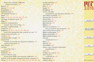
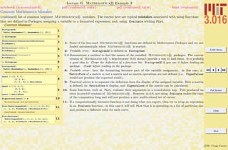
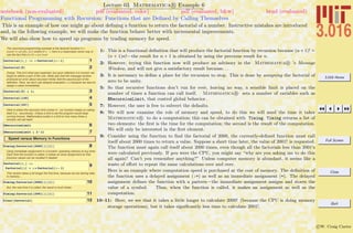
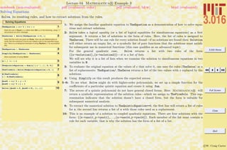
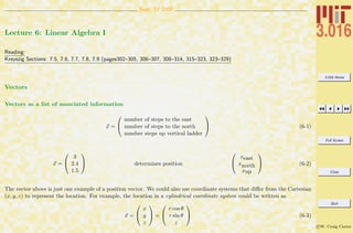
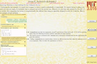
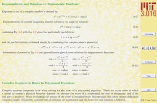
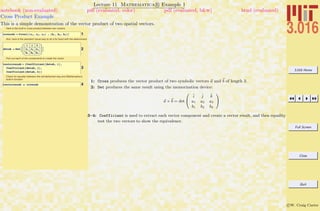
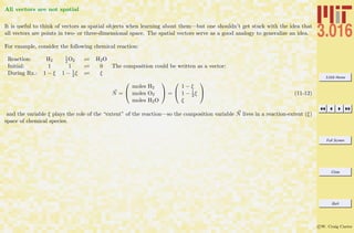
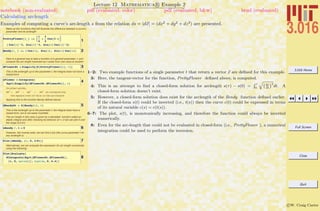
Lecture 01 Mathematica R Example 1
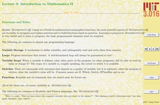
Common Mathematica Mistakes
notebook (non-evaluated) pdf (evaluated, color) pdf (evaluated, b&w) html (evaluated)
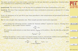
A list of common beginner Mathematica mistakes. The entries here are typical mistakes. I welcome input from others to might add
to this list
1-7 are examples of confusing usages of parentheses (—), curlies {—}, and square brackets [—]. Generally, parentheses (—) are for
logical grouping of subexpressions (i.e., (a+b)/(a-b)); curlies {—} are for forming lists or iteration-structures, single square brackets
[—] contain the argument of a function (i.e., Sin[x]), double square brackets [[—]] pick out parts of an expression or list.
Examples of Common Mistakes!
1Cos Hk xL
2Plot@Sin@xD, Hx, 0, pLD
3Sort@Hx, y, zLD
4:
2
2
> 8a, b, c<
5
SomeList = 8a, b, c, d<;
SomeList@1D
6AIz2
+ y2
M c + b y3
E a
7Exp@@1DD
8arccos@1D
9Arccos@1D
10MyFunction@x, y, zD := Sin@xD Sin@yD Sin@zD
11MyFunction@p, p ê 2, 0D
12x = p ê 2;
AbsSin@x_D = Abs@Sin@Abs@xDDD
13Plot@AbsSin@zD,
8z, -2 p, 2 p<, PlotStyle -> ThickD
1: Probable error: The parenthesis do not call a function, but would imply multiplication instead.
2: Error: The plot’s range should be in curlies {—}.
3: Error: Sort should be called on a list, which must be formed with curlies—not parenthesis.
4: Probable error: If the intention was to multiply the list by a constant, then the first set of curlies
turned the constant into a list, not a constant.
5: Probable error: If the intention was to extract the first element in the list, then double square brackets
are needed (i.e., [[—]]).
6: Error: brackets cannot be used for grouping, use parentheses instead.
7: Probable error: The double brackets do not make a function call.
8–9: Probable error: Mathematica R is case sensitive and functions are usually made by concatenating
words with their first letters capitalized (e.g., ArcCos).
10: Functions are usually created designed with patterns (i.e., x , y ) for variables. This is an error if x
is a defined variable. This line is correct in using the appropriate delayed assignment :=.
12: Probable error: Here a function is defined with a direct assignemt (=) and not delayed assignment
:=. Because x was defined previously, the function will not use the current value of x in future calls,
but the old one.

45. 3.016 Home
Full Screen
Close
Quit
c W. Craig Carter
Lecture 01 Mathematica R Example 2
Common Mathematica Mistakes
notebook (non-evaluated) pdf (evaluated, color) pdf (evaluated, b&w) html (evaluated)
(continued) list of common beginner Mathematica R mistakes. The entries here are typical mistakes involving: the difference
between assignment (=) and logical equality (==); forgetting commas; and, inadvertantly reusing a defined variable.
Common Mistakes!
The difference between assignment = and
equality testing ==
1Solve@8h = 3 p + 4 q, k = 5 p - q<, 8p, q<D
2
d ã 24
Not using enough commas
3Plot@Sin@x + Exp@-xDD 8x, 0, Pi< D
Forgetting that a variable has been defined
4
A = ‰
-1.2
k 373
Practical Advice 1:
Clear Variables
5
Clear@kD;
A = ‰
-1.2
k 373
Practical Advice 2:
Second to last resort, clear everything
6Clear@"Global`*"D;
Practical Advice 3:
Last resort, kill the kernel and restart it Use menu: Evaluation
1: Probable error: In the first line, assignments (=) are used instead of the double equals (==) which
is a logical equality.
2: Probable error Assignment of the symbol δ was probably intended by here a logical equality is queried
(i.e., Is δ the same as 24?) and no value is assigned to δ.
3: Error Commas separate arguments in functions like Plot that require at least two arguments.
4: Probable error: The symbol k was inadvertently assigned in the first line, and its value is still known
to Mathematica R .
5: Practical advice is to clear the variable definitions with Clear.
6: More powerful practical advice, but slight overkill, is to clear all user-defined variables. As a last
resort when everything seems awry, kill the kernel with the menu and restart it. This starts up a
new Mathematica R session, but does not destroy the text in the Notebook.

46. 3.016 Home
Full Screen
Close
Quit
c W. Craig Carter
Lecture 01 Mathematica R Example 3
Common Mathematica Mistakes
notebook (non-evaluated) pdf (evaluated, color) pdf (evaluated, b&w) html (evaluated)
(continued) list of common beginner Mathematica R mistakes. The entries here are typical mistakes associated with using functions
that are defined in Packages; assigning a variable to a formatted expression; and, using Evaluate withing Plot.
Common Mistakes!
1Histogram3D@
Table@8RandomReal@D, RandomReal@D<, 85<DD
2<< Histogram`
3SetDirectory@$InstallationDirectoryD
FileNames@D
4SetDirectory@"AddOns"D
FileNames@D
5SetDirectory@"Packages"D
FileNames@D
6<< Histograms`
7Histogram3D@
Table@8RandomReal@D, RandomReal@D<, 820<DD
Mistake: Using formatting commands in assignments
8
mymat = 881, 3, 7<,
83, 2, 4<,
87, 4 , 3<< êê MatrixForm
9
mymat = 8 81, 3, 7<,
83, 2, 4<,
87, 4 , 3<<;
mymat êê MatrixForm
10Eigenvalues@mymatD êê N
Not using Evaluate : slow and monochrome.
11Plot@Table@LegendreP@i, zD, 8i, 1, 11, 2<D,
8z, -1, 1<, PlotStyle Ø Thickness@0.01DD
Using Evaluate : Fast and multicolored.
12
Plot@Evaluate@
Table@LegendreP@i, zD, 8i, 1, 11, 2<DD,
8z, -1, 1<, PlotStyle Ø Thickness@0.01DD
1: Some of the less-used Mathematica R functions are defined in Mathematica Packages and are not
loaded automatically when Mathematica R is started.
2: Probable error: Histogram3D is defined in Histograms
3–6 Demonstrate a method to find the names of the installed Mathematica R packages. The current
version of Mathematica R ’s help-browser (6.0) doesn’t provide a way to find them. It is probably
a good idea to Clear the definition of a function like Histogram3D if you use it before loading its
package. Clear before reading in the package.
8: Probable error: here the formatting becomes part of the variable assignment. In this case, a
MatrixForm of a matrix is not a matrix and so matrix operations are not defined (i.e., EigenValues
would not produce the expected result).
9: Practical advice is to separate the definition from the display of the assigned variable. Here a matrix
is defined; its MatrixForm is display, and Eigenvalues of the matrix can be calculated.
10: Some functions, such as Plot, evaluate their arguments in a round-about way. This produced an
error in pre-6.0 versions of Mathematica R . However, in 6.0, not using Evaluate makes the time
of the compuation long and will not produce a nice multi-colored set of curves.
11: If a computationally intensive function is not doing what you expect, then try to wrap an expression
in an Evaluate function—in this case it will tell Plot that it is operating on a list of particular size
and produce a different color for each curve.

47. 3.016 Home
Full Screen
Close
Quit
c W. Craig Carter
Sept. 7 2007
Lecture 2: Introduction to Mathematica
Expressions and Evaluation
There are very many ways to learn how to use Mathematica R . Nearly all of the best ways involve performing examples
from the very beginning. That is how we are going to start—with examples. Using Mathematica R ’s FrontEnd you may
execute a command by pressing Shift-Enter; simply pressing Enter tells Mathematica R ’s that you merely wish to have a
“carriage return” on the screen.
Mathematica’s syntax will feel fairly natural after a while. Use the following notebook to get started. Execute a few
commands until you get a sense for what output Mathematica R will produce; try editing the commands; try to make
Mathematica R do something strange—just try playing with it and you will soon get the hang of what is going on.
One way to use Mathematica R is simply as a calculator that allows symbols to get carried along. Mathematica R will
usually try to resolve every symbol and return precise information about it. If something is undefined to Mathematica R ,
it simply returns it as a symbolic expression.
A number is not returned until all of the symbols in an expression are defined as numbers. Mathematica R will try to be
exact—it does not calculate 1
3 + 1
2 by adding 0.33333 · · · + 0.5 = 0.83333 . . ., it has an algorithm for adding rational numbers
and gives 5
6 .
Getting Started
There are a variety of ways to get Mathematica R started and these are specific to the operating system your computer
uses. A license must be purchased to run Mathematica R code, but free Mathematica R -display tools can be obtained
from Wolfram.

48. 3.016 Home
Full Screen
Close
Quit
c W. Craig Carter
The FrontEnd is the graphical interface between the user and Mathematica R —you arrange your Mathematica R
input, sometimes with text-like comments, in the FrontEnd. The user must request the FrontEnd to pass something to
Mathematica R ’s kernel, by pressing Shift-Enter. The kernel is the resident symbolic algebra software engine behind
Mathematica R .
The appearance of the FrontEnd depends on either provided or user-designed StyleSheets. The StyleSheet for this course can
be downloaded from the course website. The course style is particulary ugly—it is hoped that this will provide an incentive
for students to create their own style.
There is also a useful notebook to help you build a Palette to find documentation, tutorials, overviews, and information on
Mathematica R packages. When you have Mathematica R running, you should download this Help-Palette-Builder.nb,
open it up as as a Mathematica R notebook and follow the instructions to install the Palette that gets built.

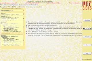
49. 3.016 Home
Full Screen
Close
Quit
c W. Craig Carter
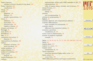
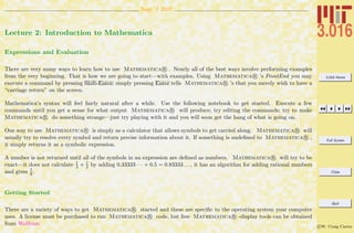
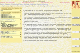
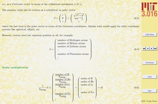
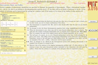
Lecture 02 Mathematica R Example 1
Basic Input and Assignment
notebook (non-evaluated) pdf (evaluated, color) pdf (evaluated, b&w) html (evaluated)
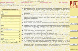
The methods of assigning symbols (SomeVariable) to expressions via SomeVariable = expr. The expr can contain other symbolic
variables, functions, programs, graphics, and many other things. There are important differences between exact (symbolic) objects and
numerical objects. Logical equalities (==) are not assignments, but are Boolean operations.
Assigning values to symbols
1a =
4 p
3
2UnitSphereVolume = a
32 a
4ANewVariable = H2 a + bL^2
5ANewVariable^2
6b =
4 H3.14159265358979L
3
7UnitSphereNumericalVolume = b
8ANewVariable
Differences between exact expressions and numerical expressions
9UnitSphereVolume - UnitSphereNumericalVolume
10a -
4 ArcCos@-1D
3
11a -
4 ArcCos@-1.0D
3
122 Pi - 2 H3.141519L
13N@5 ê 6D
Distinction between Equality (= = ) and Assignment (=)
14a ã
4 ArcCos@-1D
3
15a ã
4 H3.14159L
3
1: A symbol is assigned to an expression with an equals sign =. Some symbols, such as π, are already
defined—in Mathematica R it is exactly the ratio of a circle’s circumference to its diameter. Here,
a is a symbol that could represent, for example, the volume of a sphere with radius 1—and not an
approximation depending on how many digits are used to numerically represent π.
2: In my opinion, the variable a is not a very good name. We might forget what it represents, or
try to use it again in a different context. I think it is much better to use descriptive names,
such as UnitSphereVolume. Here, because there is an assignment in UnitSphereVolume = a,
Mathematica R tries to see if there are any other assignments associated with the right-hand-
side, and if there are it uses them until all possible assignments have been made.
3: Because no assignment was made to a just above, its value is not changed.
4: The RHS in an assignment (here to ANewVariable) can contain unassigned symbols.
6–7: Here, the symbols b and UnitSphereNumericalVolume are assigned to an approximation to the unit
sphere volume.
8: Note that, because ANewVariable contains b, the assignment of b above is reflected in the current
value of ANewVariable: Mathematica R will check to see if any symbol being output has been
assigned.
9: To show the difference between the numerical approximation of π and the symbol π, subtraction
shows that the difference is a very very small number.
10: Some functions can behave as exact if their values can be expressed exactly: here ArcCos[-1] is
exactly pi.
11: Notice that the output here is different, showing that ArcCos[-1.0] has been replaced with a numerical
representation because the function was executed on a numerical object.
14: The operator == tests to see if the LHS (left-hand side) and the RHS (right-hand side) can be
determined to be equal, in which case it returns true.
15: If == can do so, it will return false if the two sides are not equal; otherwise if it can’t say whether
true or false, it will just return the statement itself.

50. 3.016 Home
Full Screen
Close
Quit
c W. Craig Carter
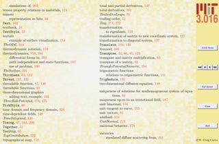
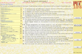
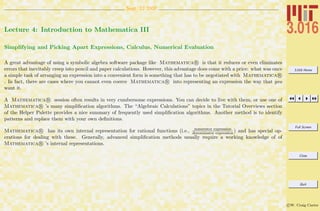
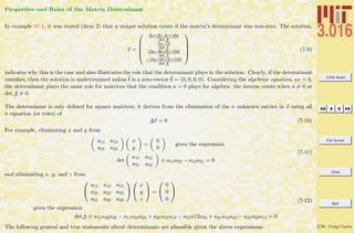
Lecture 02 Mathematica R Example 2
Building Expressions and Functions and Operations on Expressions
notebook (non-evaluated) pdf (evaluated, color) pdf (evaluated, b&w) html (evaluated)
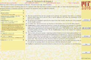
Sometimes it is easier to build up complicated expressions by entering shorter subexpressions beforehand. There are usually many ways
to do the same thing in Mathematica R , and this is demonstrated for functions. As you begin, pick the most simple method that
works. Someday later you can pick up the alternative methods—they can be useful in advanced usage.
Mathematica Functions
1a = 1 ê Exp@xD
2b = Cos@xD
3c = Ha + bL^2
Alternative Syntax for Functions (There are many ways to do the same
thing)
4AnotherVersionofb = x êê Cos
5YetAnotherVersionofb = Cosüx
6YetEvenAnotherVersionofb =
Function@z, Cos@zDD@xD
7YetStillAnotherVersionofb =
Function@Cos@ÒDD@xD
8FinallyAnotherVersionofb = HCos@ÒD &L@xD
9ANewVariable@xD
Mathematica Operations on expressions
10c
AnotherVersionofC = Expand@cD
11c
Simplify@AnotherVersionofCD
Calculus
12IntegralofC = Integrate@c, xD
13Integrate@c ê x, xD
Getting information (part 1)
14? ExpIntegralEi
1–3: This is a simple example of building up an expression piece-by-piece. For very complicated expres-
sions, this is much easier and less prone to typing errors.
4–8: One of the difficulties of learning Mathematica R is that the syntax can appear to be very
complicated and hard to remember. As you begin, just use functions in the form of Cos[x]. Here,
just as a heads-up, other ways to do the samething are presented. We will use 4 sometimes in this
course, because it is convenient. The most useful form is probably 8, this invokes the concept of a
pure function.
10–11: One of the powerful aspects of a symbolic algebra program is the manipulation of expressions.
It’s fast and it doesn’t make mistakes as one might using pencil and paper. Here are examples of
Expand (which expands all products) and Simplify (which uses an algorithm to choose among
various forms).
12–13: Another powerful aspect is the ability to perform more advanced mathematics. The integral in
12 is one that perhaps you might have been able to do after one semester of calculus; 13 is one you
would have to manipulate and look up in tables—the answer demonstrates that Mathematica R
knows about many many different functions.
14: If you see a symbol that you don’t recognize you can either use the help-browser or ask the front-
end directly. Mathematica R has a fairly consistent function naming strategy The first letter
of a word is always capitalized; compound words are concatenated together while maintaining the
first letter capitalization; thus InverseBetaRegularized. A function is just another symbol—if a
symbol is followed by square brackets [] the stuff inside the brackets become the argument(s) for
the function.

51. 3.016 Home
Full Screen
Close
Quit
c W. Craig Carter
Lecture 02 Mathematica R Example 3
Calculus and Plotting
notebook (non-evaluated) pdf (evaluated, color) pdf (evaluated, b&w) html (evaluated)
The derivative and integration methods are introduced. Simple plotting methods are demonstrated with an example of annotating a plot.
1D@ANewVariable@xD, xD
2Integrate@ANewVariable@xD, xD
3D@ANewVariable@xD, zD
4tempvar =
Integrate@ANewVariable@xD, 8x, 0, y<D
5D@tempvar, xD
6D@tempvar, yD
7Factor@IntegralofCD
8
IntegralofC
AnotherVersionofIntegralofC =
Integrate@AnotherVersionofC, xD
9c
D@IntegralofC, xD
10Factor@cD
Simplify@D@IntegralofC, xDD
11Plot@IntegralofC, 8x, 0, 10<D
12Plot@8IntegralofC, c<, 8x, 0, 10<D
13Plot@c, 8x, 0, 10<, PlotRange Ø 80, 0.0001<D
14Options@PlotD
15
Plot@8IntegralofC, c<, 8x, 0, 10<,
PlotStyle Ø 88Red, Thickness@0.005D<,
8RGBColor@0.2, 0.56, 1D,
Thickness@0.0075D<<, BaseStyle Ø
8FontFamily Ø "Helvetica", FontSize Ø 24<,
PlotLabel Ø " A Function HPretty Sky
BlueLnand Its Integral HRedLn",
AxesLabel Ø 8"Value", "Argument"<,
ImageSize Ø 800D
1: If Mathematica R can’t differentiate or integrate a function, it will be left in a symbolic form. D
is Mathematica R ’s function to take derivatives.
2: If Integrate can’t integrate a function, it will return the result in symbolic form.
3: Mathematica R is rigorous about applying the rules of calculus. . .
4: Let tempvar be the result of integrating some function of x from 0 up to some arbitrary value y—the
result should be a function of y.
5–6: Mathematica R knows about the fundamental theorems of calculus. . .
7: The calculus operations will often create long and complicated expressions. That two expressions
are equivalent can sometimes be shown with built-in functions such as Simplify, FullSimplify,
Factor, Expand, Collect, etc., but sometimes it is an art to turn an expression into an aesthetic
form.
8–10: Reassign IntegralofC to the indefinite integral of c—note, the constant of integration is set to
zero. The integration-result is not necessarily left in the most simple form.
11: This is the simplest form of Plot. The second argument is a list giving the variable and its bounds.
The first argument should have a numerical value at most of the points within the variable’s bounds.
12: These two expressions ought to be the same; however, the output-result doesn’t make this obvious.
13: Here, operations on the above expressions do show that they are same.
14: This is the simplest version of Plot—all it needs is the expression to plot and the range over which
to plot a variable—in this case x from 0 to 10.
15: If we form a list of two expressions with {–}, then we get a curve for each expression.
16: Mathematica R ’s Plot has an algorithm to set the values of y-axis if it is not specified. To specify,
one sends Plot and option in the form of a rule—here the rule is specified for PlotRange.
17: To find all the possible options for a function with their default values, the Options function provides
a way to decipher what aspects of a plot can be changed easily.
18: Here is an example with a plot title, axes labels, different colors and thickness for the curves.

52. 3.016 Home
Full Screen
Close
Quit
c W. Craig Carter
Lecture 02 Mathematica R Example 4
Lists, Lists of Lists, and Operations on Lists
notebook (non-evaluated) pdf (evaluated, color) pdf (evaluated, b&w) html (evaluated)
Lists are useful ways to keep related information together, and Mathematica R uses them extensively. Lists could be created in
Mathematica R by using the List function, but they are usually entered in with curly-brackets {} and each element of the list is
separated by commas. List elements can be about anything, even lists themselves.
1AList = :a, b, 2, 7, 9, 1.3,
p
2
, 0>
2Length@AListD
3Cos@AListD
4AList
AList@@2DD
5AList@@83, 6<DD
6AList@@-2DD
7Sort@AListD
8Select@AList, NumberQD
9Reverse@Sort@Select@AList, NumberQDDD
10Select@AList, EvenQD
11Select@AList, PrimeQD
12Perms =
Permutations@Select@AList, ExactNumberQDD
13Dimensions@PermsD
14Transpose@PermsD êê MatrixForm
15TranPerms = Transpose@PermsD;
16TranPerms@@3DD
17TranPerms@@1, 4DD
18IntList =
Table@i, 8i, 1, Length@TranPerms@@1DDD<D
19
TranPerms êê MatrixForm
TranPerms@@All, Select@IntList, OddQDDD êê
MatrixForm
1–2: Here is a simple assignment of a list to a variable and the operation of Length on the list.
3: Some functions, such as Cos here, are threadable functions; when called on a list-argument, they will
produce a list of that function applied to each list element.
4: A list’s parts (its elements) can be picked out in a variety of ways. The Part function has a shorthand
double-bracket form.
5: If the argument inside the double bracket is a list of integers, the elements corresponding to those
integers are returned.
6: Negative integers pick elements from the end of the list.
7: Sort returns a sorted list; it will also take a second argument to specify alternative sorting rules.
8–11: There are plenty of functions designed to operate on lists; here Select returns those elements for
which the second argument ( NumberQ, in 8) evaluates to True. Functions can be applied sequentially,
as in 9, and the inner-most function is applied first.
12–13: A list’s elements can be lists themselves. For example, a matrix is represented by a list of a
list. In 12, Permutations creates a list whose elements are all the permutations (which are list
themselves) of the list on which Permutations was executed. And there even are higher-dimensional
structures such as tensors. Dimensions is a useful way of learning about such structures.
14: Here, the post-fix operator for a function ( MatrixForm) is used to change the way a matrix is
displayed. Note, the result is not a matrix, but a DisplayForm of a matrix.
15: Transpose returns the result of taking a matrix and turning the rows into columns and vice-versa.
18: Table is a common way to produce a list; here, a list of integers as long as the first row of TransPerms
is produced.
19: This is a fairly advanced example of extracting the odd-numbered columns of a matrix. The list
IntList is simply the integers for each column; its odd-numbered members are selected and become
the second (i.e., column) argument of the Part selection. The first argument is All, so the entire
row is captured for each selected column.

53. 3.016 Home
Full Screen
Close
Quit
c W. Craig Carter
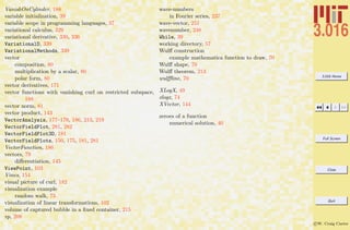
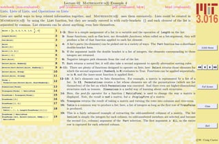
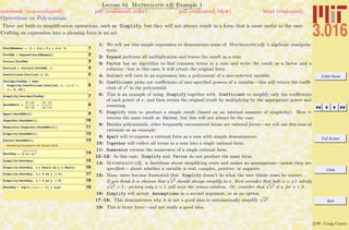
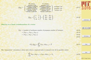
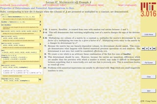
Lecture 02 Mathematica R Example 5
Rules (→) and Replacement (/.); Getting Help
notebook (non-evaluated) pdf (evaluated, color) pdf (evaluated, b&w) html (evaluated)
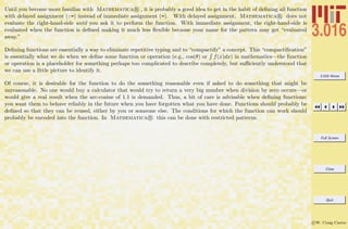
A rule leftvar → rightvar is similar to assignment in that it associates a new symbol (leftvar) with something else, but the value
is not assigned—it does not effect future values of the left-hand-side symbol. Rules are often used in conjunction with replacements and
to set options in functions. Many of Mathematica R functions, (e.g., Solve) return rules as a result.
Rules Ø and Replacement /.
1ARule = a Ø
p
3
2a
3AList
AList ê. ARule
4SomeRules = :ARule, b ->
p
12
>
5AList ê. SomeRules
6a = SomeOtherSymbol;
7AList
8StrangeRule = 8Rational@x_, y_D ß y ê x<
9HAList ê. SomeRulesL ê. StrangeRule
Getting Help: Several methods of getting help are available.
1. Typing ?ExpIntegralEi returned information about the symbol
ExpIntegralEi. Typing ??FunctionName gives even more
information~try ??Plot. Wildcards can also by used as demon-
strated below. You can click on the resulting grid-list to pull up
documentation.
10? *Exp*
Each of the above is linked to Mathematica's Help Browser.
2. Typing Options[Plot] returned a list of options that can be adjusted by
the user until the result (in this case the appearance) of the plot is
satisfactory.
Mathematica's Help Browser is a very useful tool and will probably
become a primary resource for students. It contains good tutorials and
demonstrations that can be copied and pasted. It has very good and
concise descriptions of mathematics; in fact, exploring the Help Browser
is a good way to explore mathematics as well as Mathematica. For
instance , the discussion of "Combinatorial Functions" by typing "Combi-
natorial" at the help browser---you will get a list of results that points to
tutorials and overvies.
1: The rule a → π/3 is assigned to the symbol ARule. The rule can be read as, “let a become π/3”.
2: Note, the rule does not make an assignment to the symbol a.
3: A rule can be applied with the function Replace, but the syntax (.) is typically used instead; one
can read expression/.rule as “what would expression become, if rule was applied to it.”
4–5: Rules can be collected into lists, and then applied sequentially to an expression.
6: Assignment of a will change the form of ARule, because if Mathematica R is asked for a symbol
it will make any assignments that have been called—in this case, ARule will automatically become
SomeOtherSymbol→ π/3.
7: Likewise, AList will change because it contained the symbol a.
8: This is a somewhat advanced example using patterns and delayed rules, which will be explained
later, but the point is this: Rules are necessary for manipulations in Mathematica R , but can be
used to generate “mistakes.” Think of Rule and Replace acting on an expression as “What would
the expression be if a certain rule were applied to it?” If the rule is wrong, the resulting expression
will be as well.
9: As an exercise, see if you can figure out why this list turned out like this.
10: Besides the help browser, there are ways to get help directly from the FrontEnd. Here, a list of
hyperlinks to documentation for functions containing the string “Exp” is obtained.

54. 3.016 Home
Full Screen
Close
Quit
c W. Craig Carter
Getting Help on Mathematica
With the implementation of Mathematica R 6.0, the help-browser changed considerably. Many consider it an improvement,
but I am not yet convinced—perhaps I am becoming inflexible and resistant to change.
In the old days, one would memorize large portions of the Mathematica R book—which has grown continuously heavier
since its first publication in the early 1990’s—and rely on the useful ”?” and ”??” operators. The use of ”?” with the wildcard
”” enabled a beginning user to track down almost any Mathematica R function. The Options function is also a very
efficient way to discover alternate ways of getting results.
Wolfram decided to stop updating the book as of 6.0, and it is no longer being published. When Mathematica R first came
out (I was already familiar with symbolic algebra packages like Macsyma, which predated Mathematica R ), I learned it by
reading the entire book in one sitting and then I could quickly find and reread parts as I needed it. I found this very effective,
and I am curious about what is the most effective way to learn Mathematica R today. I’d be happy to hear suggestions.
In any case, I encourage you to idly explore the Mathematica R Help-Browser. You will not only learn about Mathematica R
, but also about mathematics.

55. 3.016 Home
Full Screen
Close
Quit
c W. Craig Carter
Lecture 3: Introduction to Mathematica II
Sept. 10 2007
Functions and Rules
Besides Mathematica R ’s large set of built-in mathematical and graphics functions, the most powerful aspects of Mathematica R
are its ability to recognize and replace patterns and to build functions based on patterns. Learning to program in Mathematica R
is very useful and to learn to program, the basic programmatic elements must be acquired.
The following are common to almost any programming language:
Variable Storage A mechanism to define variables, and subsequently read and write them from memory.
Loops Program structures that iterate. A well-formulated loop will always be guaranteed to exit2.
Variable Scope When a variable is defined, what other parts of the program (or other programs) will be able to read its
value or change it? The scope of a variable is, roughly speaking, the extent to which it is available.
Switches These are commands with outcomes that depend on a quality of variable, but it is unknown, when the program is
written, what the variable’s value will be. Common names are If, Which, Switch, IfThenElse and so on.
Functions Reusable sets of commands that are stored away for future use.
All of the above are, of course, available in Mathematica R .
The following are common to Symbolic and Pattern languages, like Mathematica R .
2
Here is a joke: “Did you hear about the computer scientist who got stuck in the shower?” “Her shampoo bottle’s directions said, ‘wet hair,
apply shampoo, rinse, repeat’.”

56. 3.016 Home
Full Screen
Close
Quit
c W. Craig Carter
Patterns This is a way of identifying common structures and make them available for subsequent computation.
Recursion This is a method to define function that obtains its value by calling itself. An example is the Fibonacci number
Fn ≡ Fn−1 +Fn−2 (The value of F is equal to the sum of the two values that preceded it.) Fn cannot be calculated until
earlier values have been calculated. So, a function for Fibonacci must call itself recursively. It stops when it reaches the
end condition F1 = F2 = 1.

57. 3.016 Home
Full Screen
Close
Quit
c W. Craig Carter
Lecture 03 Mathematica R Example 1
Procedural Programming
notebook (non-evaluated) pdf (evaluated, color) pdf (evaluated, b&w) html (evaluated)
Simple programs can be developed by sequences of variable assignment.
Evaluating a sequence of instrutions (;;;)
1
a = 1;
a = a + a; a = a^a
a = a + a; a = a^a
2Clear@aD
Loops
3? Do
4a = 1; Do@a = 2 a; a = a^a, 8i, 1, 2<D
5a
6
a = 0.1; Do@a = 2 a; a = a^a;
Print@"iteration is ", i, " and a is ", aD,
8i, 1, 4<D
7Clear@aD
8? For
9
For@a = 0.1; i = 1,
i § 4, i++, a = 2 a; a = a^a;
Print@"iteration is ", i, " and a is ", aD D
10? While
11? Table
12Clear@aD
13a = 0.25;
Table@8i, a = 2 a; a = a^a<, 8i, 1, 4<D
14a = 0.75;
Table@8i, a = 2 a; a = a^a<, 8i, 1, 4<D
15
datatable = Table@
8dx, For@a = dx; i = 1, i § 4, i++, a = 2 a;
a = a^aD; Log@aD<, 8dx, 0.01, 0.5, 0.01<D
1: Here is a simple program that is just a sequence of statements that reassigns a from an initial value
(a=1). The program does this: take a add it to itself and assign the result back to a; raise this new
a to the power a and assign back to itself. Repeat. In Mathematica R , a semicolon— ;—just
indicates that output should be suppressed. There are five executions—two of them produce output
on the screen.
3: However, it would be cumbersome and unaesthetic if we wanted to generalize the last two lines to
many executions of the same type. This is where program loops come in. Do is a simple way to
loop over an expression a fixed number of times. This is equivalent to item 1, but could be easily
generalized to more iterations.
4: The Do loop does not produce intermediate output, the current value of a can be obtained by asking
Mathematica R for the current value.
5: Here an equivalent example, but extra Print statements are added so that intermediate output can
be observed.
8: A For loop is another loop structure that enforces good programming style: Its arguments provide:
an initialization, an exit condition, an iteration operator, and a function statement, and is equivalent
to item 6, but it includes (a different) initial value for a in the For statement and iterates 4 times
instead of 2.
9: The are many types of loop constructs; While is yet another.
10: Table is a very useful Mathematica R iterating function. While it iterates, it leaves intermediate
results in a List structure. Thus, the built-up list can be analyzed later.
13: Except for the intial iteration value of a, and the number of loops, this is practically equivalent to
items 1, 4, 6, and 9. We can think of this as a little program that takes an initial value of a and
returns a final value as the last member of the resulting list.
14: We could change the initial value and see how the function varies with its initial value.
15: Or, we can generalize to many initial values, by putting a Table and a For together. The result is
a list of lists (each of length 2): The first entry in each list is the initial value (dx) and the second
entry is the result of the For-loop after four iterations for that dx. Because the values tend to get
very large, we wrap a Log (natural log) around the result of the For-loop. A special increment
structure is utilized—it sets initial and final values as well as the increment size.

58. 3.016 Home
Full Screen
Close
Quit
c W. Craig Carter
Lecture 03 Mathematica R Example 2
Plotting Lists of Data and Examples of Deeper Mathematica R Functionality
notebook (non-evaluated) pdf (evaluated, color) pdf (evaluated, b&w) html (evaluated)
This demonstrates how visualizing data can be combined with other functions to perform analysis. Here, we show that the little iterative
program produces a minimum and then we analyze the minimum with two different methods.
1ListPlot@datatableD
2Options@ListPlotD
Note that the options are written as Rules.
3ListPlot@datatable, PlotRange Ø 8250, 500<,
PlotStyle Ø PointSize@0.025DD
4? *Minimum*
5
FindMinimum@For@a = xvalue;
i = 1, i § 4, i++, a = 2 a; a = a^aD;
Log@aD, 8xvalue, 0.15, 0.25<D
By going into the Help Browser, you can see that the output of FindMini-
mum is a list, the first element of which is the functions minimum value,
and the second is a Rule specifing where the minimum occurs.
Lets try and do the above the hard way. I will use Nest to recursively
apply the function 4 times (I am just using a shorthand here, we can
ignore the use of Nest for this course...). You can see that it works. Don't
worry about it, but if you want to know about it, use the Help Browser to
get information about Nest and Pure Functions.
6Clear@xD
7fx = Nest@H2 ÒL^H2 ÒL &, x, 4D
Take it derivative and set equal to zero...
8dfx = D@fx, xD êê Simplify
Finding the zero of this will not be easy.... but FindRoot claims it can do
it...
9FindRoot@dfx, 8x, .1, .3<D
1: The data produced from the last example can be plotted. It is apparent that there is a minimum
between initial values of 0.1 and 0.3. But, it will be difficult to see unless the visualization of the
plot can be controlled.
3: By specifying the ListPlot’s option for the range of the y-like variable, the character of the minimum
can be visually assessed.
4: It is likely that Mathematica R has functions to find minima; here we look for likely suspects.
5: FindMinimum is a fairly sophisticated function to obtain the minimum of an expression in a specified
range, even if the function only returns a numerical result. Here FindMinimum is used, to find a very
high precision approximation to the minimum observed in item 3. The function is our For-loop with
a variable xvalue as the initial value. We ask FindMinimum to hunt for the xvalue that minimizes
the ( Log of the) For-loop.
7: This is a fairly advanced example—beginning students should not worry about understanding it yet.
Nest is a sophisticated method of repeated applications of a function (i.e., f(f(f(x))) is nesting the
function f three times on an argument x). It is equivalent to the previous methods of producing the
iterative structure, but now the result is an expression with a variable x that plays the role of the
initial value. This concept uses Pure Functions which are produced by the ampersand &.
8: The minimum of the function can be analyzed the standard way, here by taking derivatives with D.
It would not be amusing (that is, for most of us) to find this derivative by hand.
9: FindRoot is sophisticated numerical method to obtain the zero of an expression in a specified range.

59. 3.016 Home
Full Screen
Close
Quit
c W. Craig Carter
Very complex expressions and concepts can be built-up by loops, but within Mathematica R the complexity can be buried
so that only the interesting parts are apparent and shown to the user.
Sometimes, as complicated expressions are being built up, intermediate variables are used. Consider the value of i after
running the program:
FindMinimum[For[a = dx; i = 1, i ≤ 4, i++, a = 2a; a = a∧a]; Log[a], {dx, 0.15, 0.25}]; the value of i (in
this case 5) has no useful meaning anymore. If you had defined a symbol such as x = 2i previously, then x would now have
the value of 10, which is probably not what was intended. It is much safer to localize variables—in other words, to limit
the scope of their visibility to only those parts of the program that need the variable and this is demonstrated in the next
example. Sometimes this is called a “Context” for the variable in a programming language; Mathematica R has contexts
as well, but should probably be left as an advanced topic.

60. 3.016 Home
Full Screen
Close
Quit
c W. Craig Carter
Lecture 03 Mathematica R Example 3
Making Variables Local and Using Switches to Control Procedures
notebook (non-evaluated) pdf (evaluated, color) pdf (evaluated, b&w) html (evaluated)
Describes the use of Module to “hide” a variable: consider the variable a from the first item in the above example—its intermediate
values during iteration are not always important. Suppose you wish to use the symbol a later, that it played an intermediate role hence
was not used, and may easily be forgotten. It is good practice to make such variables ‘local’ to their own functions.
An example of a logical switch is demonstrated for If.
Local Variables
1xvalue
a
2CurrentValueofA = a;
3
xvalue = SnickerDoodle; a = HappyGoLucky;
Module@
8xvalue, a, maxiteration = 4, solution, i<,
solution =
FindMinimum@For@a = xvalue; i = 1,
i § maxiteration, i++, a = 2 a; a = a^aD;
Log@aD, 8xvalue, 0.15, 0.25<D;
Print@xvalue ê. solution@@2DDD
D
4
xvalue
a
solution
Switches: If, Which
5a = Prime@23D + Prime@62D + Prime@104D
6
If@PrimeQ@aD,
Print@a , " is a Prime Number"D,
Print@a,
" is not Prime, its divisors are ",
Divisors@aDD,
Print@"I have no idea what
you are asking me to do!"D
D
The above program is ok, but not very useful because it only works for
the current value of a. It would be more useful to have something that
worked for any value of a and could use it over again~that is, turn it into
a tool. This involves patterns and function definitions.
1: The symbols xvalue and a are left over from the last example, even though they played only an
intermediate role for the final result. It is not unusual to run the same Mathematica R for a day
or more—it would be easy to forget that values have been assigned to symbols.
2: This could lead us to mistakenly use its value later as though it might be undefined. This is a
common error.
3: The production of such errors can be reduced with a programming practice known as localized
variables (also known as variable-scoping). The idea is to hide the variable within its own structure—
the variable is said to have a limited scope. Module provides a function for doing this. Here symbols
xvalue and a have set values before the call to Module, but any value that is changed inside of Module
has no effect on its “global” value in the rest of the Mathematica R session.. Using Module is
good programming practice for creating your own functions.
4: Even though Module changed the symbols xvalue and a, and used an internal variable solution,
there should be no effect outside of Module.
6: It is useful to build functions that are “smart” (or appear to be so, by applying rules of logic). Here,
a simple example of the use of If will be applied to a symbol which is the sum of the 23rd
, 62nd
,
and 104th
prime numbers.
This is a simple program. First, it checks if a is prime using the query-function PrimeQ. If the check
is true, then it prints a message saying so, and then returns control to the Mathematica R kernel.
If the check is false, then it prints out a message and some more useful information about the fact
it isn’t prime using Divisors. If the statement cannot be determined to be true or false, a message
to that effect is printed.

61. 3.016 Home
Full Screen
Close
Quit
c W. Craig Carter
Patterns are extremely important in mathematics and in Mathematica R . The goal for beginners should be to master how to
create your own functions: understanding how to use patterns is essential to creating your own functions in Mathematica R
.
In Mathematica R , the use of the underscore, , means “this is a placeholder for something that will be used later.”3 In
other words, you may want to perform a predictable action on an object (e.g., find the value of its cosine, determine if it is
prime, plot it), but want to create the action before the object exists. We create the action using a pattern ( ), the arbitrary
object, and create fixed operations on the pattern.
Usually, one needs to name the pattern to make it easier to refer to later. The pattern gets named by adding a head
to the underscore, such as SomeVariableName , and then you can refer to whatever pattern matched it with the name
SomeVariableName.
This is a bit abstract and probably difficult to understand without the aid of a few examples. We start with patterns and
replacement in the following example, and then build up to functions in the next example.
3
It is a bit like teaching a dog to fetch—you cock an arm as if to throw something , and then when something gets thrown, your dog runs
after the “something.” The first something is a place holder for an object, say anything from a stick to a ball to the morning paper. The second
something is the actual object that is actually tossed, that finally becomes the “something” your dog uses as the actual object in the performance
of her ritual response to the action of throwing.

62. 3.016 Home
Full Screen
Close
Quit
c W. Craig Carter
Lecture 03 Mathematica R Example 4
Operating with Patterns
notebook (non-evaluated) pdf (evaluated, color) pdf (evaluated, b&w) html (evaluated)
Patterns are identified by the underscore , and the matched pattern can be named for later use (e.g., thematch ).
1AList = 8first, second,
third = 2 first, fourth = 2 second<
2AList ê. 82 a_ Ø a<
3Clear@aD
4AList ê. 82 a_ Ø a<
5
AList ê.
8p_ , q_ , r_ , s_< Ø 8p , p q, p q r, p q r s<
682, 0.667, a ê b, Pi< ê. 8p_Integer Ø p One<
_ all by itself stands for anything. x_ also stands for anything, but gives
anything a name for later use.
7AList ê. _ Ø AppleDumplings
8PaulieNoMealX = Sum@b@iD x^i, 8i, 2, 6<D
9PaulieNoMealX ê. x^n_ Ø n x^Hn - 1L
Make the rule work for any polynomial...
10DerivRule = q_^n_ Ø n q^Hn - 1L;
11PaulineOMealY = Sum@c@iD z^i, 8i, 2, 6<D
12PaulineOMealY ê. DerivRule
PaulieNoMealX ê. DerivRule
Another problem is that it will not work for first-order and zeroeth-order
terms...
13PaulENoMiel = Sum@c@iD HoneyBee^i, 8i, 0, 6<D
14PaulENoMiel ê. DerivRule
This could be fixed, but it would be much easier to do so by defining
functions of a pattern.
It is also possible to have a pattern apply conditionally.
15
Cases@881, 2<, 82, 1<, 8a, b<, 82, 84<, 5<,
8first_, second_< ê; first < secondD
1: Construct an example AList = {first, second, 2first, 2second} to demonstrate use of pattern
matching. We will try to replace members that match 2 something with something There is an
instructive error in the first try.
2: The rule is applied to AList through the use of the operator /. (short-hand for ReplaceAll). The
pattern here is “two multiplied by something.” The symbol a should a placeholder for something,
but a was already defined and so the behavior is probably not what was wanted: 2 something was
replaced by the current value of a. Another (probably better, but better left until later) usage is the
delayed ruleset :->.
4: After a has been cleared, the symbol a is free to act as a placeholder. In other words, a takes on the
temporary value of the last match. The effect of applying the rule is 2×all somethings are replaced
by the pattern represented by a which takes a temporary value of each something.
5: Here is an example that uses each member of a four-member list, names the members, and then uses
a rule to operate on the entire list. Study this example until you understand it.
6: The types of things that get pattern-matched can be restricted by adding a pattern qualifier to the
end of the underscore. Here, we restrict the pattern matching to those objects that are Integer. The
first replacement makes sense; however, the third member of the list is understood by considering
that the internal representation of a/b is a×Power[b,-1]—the -1 is what was matched.
7: It is not necessary to name a pattern, but it is a good idea if the match is to be used again later.
Here, the first thing that gets matched (the list itself) is replaced with the new symbol.
8: For a simple (incomplete and not generally useful) example of the use of patterns, an example
producing symbolic derivative of a polynomial will be developed. Here, a polynomial PaulNoMealX
in x is defined using Sum.
9–10: A rule is applied, which replaces patterns x to a power with a derivative rule. If only the power is
used later, so it is given a place-holder name n. This technique would only work on polynomials in
x. To generalize (10), we need a place-holder for the arbitrary variable and its powers.
13–14: This will not work for the constant and linear terms in a polynomial. This could be fixed, but the
example becomes complicated and still not as good as Mathematica R ’s built-in differentiation
rules.
15: To place more control on the types of patterns that get matched, patterns can also be used in
conjunction with Condition operator /;. Here is an example of its use in Cases. The pattern is
any two-member list subject to the condition that the first member is less than the second. Cases
returns those members of the list where the pattern was successfully matched.

63. 3.016 Home
Full Screen
Close
Quit
c W. Craig Carter
Lecture 03 Mathematica R Example 5
Creating Functions using Patterns and Delayed Assignment
notebook (non-evaluated) pdf (evaluated, color) pdf (evaluated, b&w) html (evaluated)
Understanding this example is important for beginners to Mathematica R !
The real power of patterns and replacement is obtained when defining functions. Examples of how to define functions are presented.
Defining Functions with Patterns
Defining functions with patterns probably combines the most useful
aspects of Mathematica. Define a function that takes patten matching x
as its first argument and an argument matching n as its second argument
and returns x to the nth
power:
1
f@x_ , a_D = x^a;
H*This is not a good way to define
a function, we will see why later*L
2f@2, 3D
f@y, zD
This works fine, but suppose we had defined x ahead of time
3x = 4
4
f@x_ , a_D = x^a;
H*This is not a good way to define
a function, we will see why later*L
5
f@2, 3D H*will now be 4^3,
which is probably not what
the programmer had in mind*L
6f@y, zD
Better Functions with Delayed Assignment (:=)
7x = 4
a = ScoobyDoo
8f@x_ , a_D := x ^a
9f@2, 5D
10f@y, zD
11f@x, aD
12f@a, xD
13Clear@fD
1: Here is an example of a pattern: a symbol f is defined such that if it is called as a function with a
pattern of two named arguments x and a , then the result is what ever xa
evaluated to be when
the function was defined. Don’t emulate this example—it is not usually the best way to
define a function. In words you are telling Mathematica R , “any time you see f[thing,doodad]
replace it with the current value of thingˆdoodad.”
2: Our example appears to work, but only because our pattern variables, x and a had no previous
assignment.
3–6 This shows why this can be a bad idea. f with two pattern-arguments, is assigned when it is defined,
and therefore if either x or a was previously defined, then the definition will permanently reflect that
definition. The =-assignment is performed immediately and anything on the right-hand-side will be
evaluated with their immediate values.
7–12: What we really want to tell Mathematica R in words is, “I am going to call this function in the
future. I want to define the function now, but I don’t want Mathematica R to evaluate it until it
is called; use the pattern-matching variables when you evaluate it later.” This involves use delayed
assignment which appears as :=.
For beginning users to Mathematica R , this is the best way to define functions.
In a delayed assignment, the right-hand-side is not evaluated until the function is called and then the
patterns become transitory until the function returns its result. This is usually what we mean when
we write y(x) = ax2
mathematically—if y is given a value x, then it operates and returns a value
related to that x and not any other x that might have been used earlier.
This is the prototype for function definitions.

64. 3.016 Home
Full Screen
Close
Quit
c W. Craig Carter
Until you become more familiar with Mathematica R , it is probably a good idea to get in the habit of defining all function
with delayed assignment (:=) instead of immediate assignment (=). With delayed assignment, Mathematica R does not
evaluate the right-hand-side until you ask it to perform the function. With immediate assignment, the right-hand-side is
evaluated when the function is defined making it much less flexible because your name for the pattern may get “evaluated
away.”
Defining functions are essentially a way to eliminate repetitive typing and to “compactify” a concept. This “compactification”
is essentially what we do when we define some function or operation (e.g., cos(θ) or f(x)dx) in mathematics—the function
or operation is a placeholder for something perhaps too complicated to describe completely, but sufficiently understood that
we can use a little picture to identify it.
Of course, it is desirable for the function to do the something reasonable even if asked to do something that might be
unreasonable. No one would buy a calculator that would try to return a very big number when division by zero occurs—or
would give a real result when the arc-cosine of 1.1 is demanded. Thus, a bit of care is advisable when defining functions:
you want them to behave reliably in the future when you have forgotten what you have done. Functions should probably be
defined so that they can be reused, either by you or someone else. The conditions for which the function can work should
probably be encoded into the function. In Mathematica R this can be done with restricted patterns.

65. 3.016 Home
Full Screen
Close
Quit
c W. Craig Carter
Lecture 03 Mathematica R Example 6
Functional Programming with Recursion: Functions that are Defined by Calling Themselves
notebook (non-evaluated) pdf (evaluated, color) pdf (evaluated, b&w) html (evaluated)
This is an example of how one might go about defining a function to return the factorial of a number. Instructive mistakes are introduced
and, in the following example, we will make the function behave better with incremental improvements.
We will also show how to speed up programs by trading memory for speed.
The canonical programming example is the factorial function n! =
(n)!(n-1) !(n-2)!—!(1) where 0! ª 1; here is a reasonably clever way to
use the fact that (n+1)! = (n+1)!n!
1factorial@n_D := n factorial@n - 1D
2factorial@8D
Ooops, This isn't what was expected, but upon reflection it is correct--we
forgot to define a part of the rule. (Note also that the message window
produced an error about recursion limits) Add the second part of the
definition. Here, we don't use delayed evaluation (:=) because we want to
assign a value immediately.
3factorial@0D = 1;
4factorial@120D
5factorial@257D
Here is where the recursion limit comes in : our function keeps on calling
itself (i.e., recursively). Unless a limit is set the program would keep
running forever. Mathematica builds in a limit to how many times a
function will call itself:
6$RecursionLimit
7$RecursionLimit = 2^11
Speed versus Memory in Functions
8Timing@factorial@2000DD@@1DD
Using immediate assignment in a function: spending memory to buy time:
Each time the function is called, it makes an extra assignment so that
previous values can be recalled if needed.
9
factorial@n_D :=
factorial@nD = n * factorial@n - 1D
This version takes a bit longer the first time, because we are storing data
in memory ...
10Timing@factorial@2000DD@@1DD
But, the next time it is called, the result is much faster.
11Timing@factorial@2001DD@@1DD
12Clear@factorialD
1: This is a functional definition that will produce the factorial function by recursion because (n+1)! =
(n + 1)n!—the result for n + 1 is obtained by using the previous result for n.
2: However, trying this function now will produce an advisory in the Mathematica R ’s Message
Window, and will not give a satisfactory result because. . .
3: It is necessary to define a place for the recursion to stop. This is done by assigning the factorial of
zero to be unity.
5: So that recursive functions don’t run for ever, leaving no way, a sensible limit is placed on the
number of times a function can call itself. Mathematica R sets a number of variables such as
$RecursionLimit, that control global behavior.
7: However, the user is free to subvert the defaults.
8: We will now examine the role of memory and speed, to do this we will need the time it takes
Mathematica R to do a computation; this can be obtained with Timing. Timing returns a list of
two elements: the first is the time for the computation; the second is the result of the computation.
We will only be interested in the first element.
9: Consider using the function to find the factorial of 2000, the currently-defined function must call
itself about 2000 times to return a value. Suppose a short time later, the value of 2001! is requested.
The function must again call itself about 2000 times, even though all the factorials less than 2001’s
were calculated previously. If you were the CPU, you might say “why are you asking me to do this
all again? Can’t you remember anything?” Unless computer memory is abundant, it seems like a
waste of effort to repeat the same calculations over and over.
Here is an example where computation speed is purchased at the cost of memory. The definition of
the function uses a delayed assignment (:=) as well as an immediate assignment (=). The delayed
assignment defines the function with a pattern—the immediate assignment assigns and stores the
value of a symbol. Thus, when the function is called, it makes an assignment as well as the
computation.
10–11: Here, we see that it takes a little longer to calculate 2000! (because the CPU is doing memory
storage operations), but it takes significantly less time to calculate 2001!.

66. 3.016 Home
Full Screen
Close
Quit
c W. Craig Carter
Lecture 03 Mathematica R Example 7
Restricted and Conditional Pattern Matching
notebook (non-evaluated) pdf (evaluated, color) pdf (evaluated, b&w) html (evaluated)
Here are demonstrations of how to restrict whether a pattern gets matched by the type of the argument and how to place further
restrictions on pattern matching.
Restrictions on Patterns
The factorial function is pretty good, but not foolproof as the next few
lines will show.
1Clear@factorialD
2
factorial@0D = 1;
factorial@n_D := n * factorial@n - 1D
The next line will cause an error to appear on the message screen.
3factorial@PiD
The remedy is to restrict the pattern:
4Clear@factorialD
5
factorial@0D = 1;
factorial@n_IntegerD := n * factorial@n - 1D
This time it doesn' t produce an error, and returns a value indicating that
it is leaving the function in symbolic form for values it doesn' t know about.
6factorial@PiD
Functions and Patterns with Tests
However, the definition of factorial still needs some improvement--the
next line will cause an error.
7factorial@-5D
8Clear@factorialD
9
factorial@0D = 1;
factorial@n_Integer ?PositiveD :=
n * factorial@n - 1D
10factorial@12D
11factorial@PiD
3: However, what if the previously-defined factorial function were called on a value such as π? It would
recursively call (π − 1)! which would call (π − 2)! and so on. Thus, this execution would be limited
by the current value of $RecursionLimit.
This potential misuse can be eliminated by placing a pattern restriction on the argument of factorial
so that it is only defined for integer arguments.
5: Here is an improved definition for the factorial function using a pattern type: Integer. The type-
qualifier at the end of the “ ” is the internal representation of whatever the argument was (e.g.,
Integer, Real, Complex, List, Symbol, Rational, etc.). In this case, the factorial function is
only defined for integer arguments.
6: Now the function should indicate that it doesn’t have anything further to do with a non-integer
argument.
7: However, the definition is still not fool-proof because negative integers will not terminate the recursion
properly.
9: A pattern can have conditional matching indicated by the ?Query where Query returns true for the
conditions that the pattern can be matched (e.g., Positive[2], NonNegative[0], NumberQ[1.2],
StringQ[”harpo”] all return True.) In this example, the function’s pattern—n Integer?Positive—
might be understood in words as “Match any integer and then test and see if that integer is positive;
if so use n as a temporary placeholder for that positive integer.”

67. 3.016 Home
Full Screen
Close
Quit
c W. Craig Carter
Lecture 03 Mathematica R Example 8
Further Examples of Conditional Pattern Matching; Conditional Function Definitions
notebook (non-evaluated) pdf (evaluated, color) pdf (evaluated, b&w) html (evaluated)
A simple example of patterns is demonstrated with graphics. Another method of using conditions is demonstrated.
As a another example, let's define the Sign function. It should be -1 when
its argument is negative, 0 when its argument is zero, and +1 when its
argument is positive. There are lots of ways to write this function, there is
no best way. Whatever works is good.
1? Sign
Here we write our own version, we don' t "name'' the pattern because it is
not needed in the function definition. It is a bit harder to read this way,
but I use it here to be instructive.
2
HeyWhatsYourSign@0D = 0;
HeyWhatsYourSign@0.0D = 0;
HeyWhatsYourSign@_?PositiveD := 1;
HeyWhatsYourSign@_?NegativeD := -1;
3Plot@HeyWhatsYourSign@argumentD,
8argument, -p, ‰<, PlotStyle Ø ThickD
4
Plot@81 ê x, HeyWhatsYourSign@xD ê x<,
8x, -1, 1<,
BaseStyle Ø
8FontSize Ø 18, FontFamily Ø "Helvetica"<,
PlotStyle Ø 88Hue@1D, Thickness@0.02D<,
8Hue@0.66D, Thickness@0.01D<<D
Functions with Conditional Definitions
In thermodynamics, x ln(x) appears frequently in expressions that involve
entropy. The variable x is restricted to 0 §x§1.
5
XLogX@x_D := x Log@xD ê; Hx > 0 && x § 1L
XLogX@0D = XLogX@0.0D =
Limit@xsmall Log@xsmallD, xsmall Ø 0D
6XLogX@1.2D
7Plot@XLogX@xD + XLogX@1 - xD,
8x, -1, 2<, PlotStyle Ø ThickD
1: As an example, we will try to duplicate Mathematica R ’s definition of Sign.
2: Because we want our function to return zero when it gets called with an argument of zero—exact or
numerical, immediate assignment is used in the first two lines. (It would probably be better to use
the ? PossibleZeroQ pattern match here, but slower.)
Because, we don’t need to use the value of the matched pattern we can get by without naming it
(i.e., ?Positive). I include this for instruction purposes—if I were writing this function for later
use, I’d probably go ahead and name the pattern for readability.
3: We Plot our function to see if it behaves properly. We use Plot’s option PlotStyle->Thick to
make the curve easier to see.
4: Here is an example using our function and plotting two curves with more plotting options.
5: The ideal molar entropy of mixing is the sum of Xi ln Xi for each component i with composition
Xi. Because the composition variables are limited to 0 ≤ Xi ≤ 1, our example ideal molar entropy
function should reflect this constraint.
Here we use a conditional definition (/;), to ensure that our X ln X function is never called for any
X that are out-of-bounds. The delayed assignment statement LHS := RHS/;test might be read as,
“If the symbol LHS is called, then evaluate (using whatever patterns might appear in LHS) whether
test is true; if true, then evaluate RHS with the appropriate pattern replacements.” Note that here,
we make X = 0 a special case and not included in our delayed assignment of the function.
Because ln x → −∞ as x → 0, it may not be obvious that x ln x → 0 as x → 0. We use Limit to
determine this behavior and use immediate assignment in our function definition. (This is a case
where immediate assignment makes sense; with delayed assignment the Limit function would be
called each time that XLogX is called on a zero-argument.
7: This is a plot of the ideal molar entropy of mixing for a binary alloy.

68. 3.016 Home
Full Screen
Close
Quit
c W. Craig Carter
Sept. 12 2007
Lecture 4: Introduction to Mathematica III
Simplifying and Picking Apart Expressions, Calculus, Numerical Evaluation
A great advantage of using a symbolic algebra software package like Mathematica R is that it reduces or even eliminates
errors that inevitably creep into pencil and paper calculations. However, this advantage does come with a price: what was once
a simple task of arranging an expression into a convenient form is something that has to be negotiated with Mathematica R
. In fact, there are cases where you cannot even coerce Mathematica R into representing an expression the way that you
want it.
A Mathematica R session often results in very cumbersome expressions. You can decide to live with them, or use one of
Mathematica R ’s many simplification algorithms. The “Algebraic Calculations” topics in the Tutorial Overviews section
of the Helper Palette provides a nice summary of frequently used simplification algorithms. Another method is to identify
patterns and replace them with your own definitions.
Mathematica R has its own internal representation for rational functions (i.e., numerator expression
denominator expression ) and has special op-
erations for dealing with these. Generally, advanced simplification methods usually require a working knowledge of of
Mathematica R ’s internal representations.

69. 3.016 Home
Full Screen
Close
Quit
c W. Craig Carter
Lecture 04 Mathematica R Example 1
Operations on Polynomials
notebook (non-evaluated) pdf (evaluated, color) pdf (evaluated, b&w) html (evaluated)
There are built-in simplification operations, such as Simplify, but they will not always result in a form that is most useful to the user.
Crafting an expression into a pleasing form is an art.
1PaulENomeal = H1 + 2 a + 3 x + 4 zL^4
2FatPEN = Expand@PaulENomealD
3Factor@FatPEND
4PaulinX = Collect@FatPEN, xD
5Coefficient@PaulinX, x, 2D
6
PaulSpiffedUp = Sum@
Simplify@Coefficient@PaulinX, x, iDD x^i,
8i, 0, 20<D
7Simplify@PaulSpiffedUpD
8RashENell =
Hx + yL
Hx - yL
+
Hx - yL
Hy + xL
9Apart@RashENellD
10Together@RashENellD
11Numerator@Together@RashENellDD
12Simplify@RashENellD
13Factor@RashENellD
Simplfiying Expressions with Square Roots
14RootBoy = Hx + yL2
15Simplify@RootBoyD
16Simplify@RootBoy, x œ Reals && y œ RealsD
17Simplify@RootBoy, x ¥ 0 && y ¥ 0D
18Simplify@RootBoy, x < 0 && y < 0D
19RootBoy ê. Sqrt@Hexpr_L^2D Ø expr
1: We will use this simple expression to demonstrate some of Mathematica R ’s algebraic manipula-
tions.
2: Expand performs all multiplication and leaves the result as a sum.
3: Factor has an algorithm to find common terms in a sum and write the result as a factor and a
cofactor—but in this case, it will return the original form.
4: Collect will turn in an expression into a polynomial of a user-selected variable.
5: Coefficient picks out coefficients of user-specified powers of a variable—this will return the coeffi-
cient of x2
in the polynomial.
6: This is an example of using Simplify together with Coefficient to simplify only the coefficients
of each power of x, and then return the original result by multiplying by the appropriate power and
summing.
7: Simplify tries to produce a simple result (based on an internal measure of simplicity). Here it
returns the same result as Factor, but this will not always be the case.
8: Besides polynomials, other frequently encountered forms are rational forms—we will use this sum of
rationals as an example.
9: Apart will re-express a rational form as a sum with simple denominators.
10: Together will collect all terms in a sum into a single rational form.
11: Numerator returns the numerator of a single rational form.
12–13: In this case, Simplify and Factor do not produce the same form.
14: Mathematica R is fastidious about simplifying roots and makes no assumptions—unless they are
specified— about whether a variable is real, complex, positive, or negative.
15: Many users become frustrated that Simplify doesn’t do what the user thinks must be correct. . .
If you think it is obvious that
√
x2 should always simplify to x, then consider that both x = ±1 satisfy√
x2 = 1—picking only x = 1 will miss the minus-solution. Or, consider that
√
x2 = x for x < 0
16: Simplify will accept Assumptions as a second argument, or as an option.
17–18: This demonstrates why it is not a good idea to automatically simplify
√
x2.
19: This is brute force—and not really a good idea.

70. 3.016 Home
Full Screen
Close
Quit
c W. Craig Carter
Lecture 04 Mathematica R Example 2
A Second Look at Calculus: Limits, Derivatives, Integrals
notebook (non-evaluated) pdf (evaluated, color) pdf (evaluated, b&w) html (evaluated)
Examples of Limit and calculus with built-in assumptions
1AMessyExpression =
Log@x Sin@xDD
1
x
2Limit@AMessyExpression, x Ø 0D
3DMess = D@AMessyExpression, xD
4Integrate@DMess, xD
5DefInt1 = Integrate@DMess, 8x, 0, ‰<D
6HAMessyExpression ê. x Ø eL -
HAMessyExpression ê. x Ø 0L
7DefInt2 = HAMessyExpression ê. x Ø ‰L -
Limit@AMessyExpression, x Ø 0D
8
DefInt1
DefInt2
DefInt1 ã DefInt2
9Integrate@Sin@xD ê Sqrt@Hx^2 + a^2LD, xD
10Integrate@Sin@xD ê Sqrt@Hx^2 + a^2LD,
x, Assumptions Ø Re@a^2D > 0D
11
UglyInfiniteIntegral =
Integrate@Sin@xD ê Sqrt@Hx^2 + a^2LD,
8x, 0, ¶<, Assumptions Ø Re@a^2D > 0D
12N@UglyInfiniteIntegral ê. a Ø 1D
13Series@AMessyExpression, 8x, 0, 4<D
14FitAtZero =
Series@AMessyExpression, 8x, 0, 4<D êê Normal
15
Plot@
8AMessyExpression, FitAtZero<, 8x, 0, 3<,
PlotStyle Ø 88Thickness@0.02D, Hue@1D<,
8Thickness@0.01D, Hue@0.5D<<D
1–2: This would be a challenging limit to find for many first-year calculus students (try it!).
3–4: Here, do a quick verification using differentiation and integration to check if Mathematica R agrees
with the fundamental theorem of calculus ( Integrate[ D[expr,x],x]==x). Note, Mathematica R
does not add the arbitrary constant to the indefinite integral.
5: This definite integral should the value of AMessyExpression at x = e, but is not obvious by inspection.
6: Simply evaluating (via application of rules) the integral at the ends of the integration domain does
not produce the correct result because of a possible division by zero.
7: Using Limit instead of direct evaluation produces the expected result.
8: Although they have different forms (and one can probably see that they are the same expression),
testing equality shows that the two different forms of the definite integral are the same.
9-10: Some indefinite integrals do not have closed-form solutions as in 9, even with extra assumptions
as attempted in 10.
12: But, in some cases even if the indefinite integral does not have a closed-form solution, the definite
integral will have one.
13: Series is one of the most useful and powerful Mathematica R functions; especially to replace a
complicated function with a simpler approximation in the neighborhood of a point.
Series returns a SeriesData-form which is indicated by the trailing order function O. Subsequent
operations, such as Simplify, won’t work on a SeriesData-form, but Normal converts a SeriesData
to a normal expression by chopping off the O.
14–15: In this example, FitAtZero is a fourth-order approximation to AMessyExpresssion at x = 0 and
has been converted with Normal so it can be plotted in 15 alongside the exact expression.

71. 3.016 Home
Full Screen
Close
Quit
c W. Craig Carter
Lecture 04 Mathematica R Example 3
Solving Equations
notebook (non-evaluated) pdf (evaluated, color) pdf (evaluated, b&w) html (evaluated)
Solve, its resulting rules, and how to extract solutions from the rules.
Solving Equations
1TheEquation = a x^2 + b x + c
Note the use of Equal (==) rather than Set (=) in the following; using "="
will produce an error message.
2TheZeroes = Solve@TheEquation == 0, xD
Note that the roots are given as Rules. Now we ask Mathematica to
verify that the solutions it found are indeed roots to the specified equa-
tion. Here is a prototypical example of using Replace (/.) to accomplish
this:
3TheEquation ê. TheZeroes
4Simplify@TheEquation ê. TheZeroesD
More examples of using Solve:
5a@i_D := i + 1
6TheQuinticEquation = Sum@a@iD x^i, 8i, 0, 5<D
7TheFiveSols = Solve@TheQuinticEquation ã 0, xD
8N@TheFiveSolsD
x ê. N@TheFiveSolsD
9Quad1 = a x^2 + y + 3
Quad2 = a y^2 + x + 1
10Solve@8Quad1 ã 0, Quad2 ã 0<, 8x, y<D
1: We assign the familiar quadratic equation to TheEquation as a demonstration of how to solve equa-
tions and extract solutions.
2: Solve takes a logical equality (or a list of logical equalities for simultaneous equations) as a first
argument. It returns a list of solutions in the form of rules. Here, the list of rules is assigned to
TheZeroes. There will be one rule for every solution found—if no solutions are found then Solution
will either return an empty list, or a symbolic list of pure functions that the solutions must satisfy
for subsequent use in numerical functions (this case qualifies as an advanced topic).
For the general quadratic case, Solve returns a list with two rules of the form
{{x->solution1},{x->solution2}}—it is a list of lists.
We will see why it is a list of lists when we examine the solution to simultaneous equations in two
variables in 9.
3: To evaluate the original equation at the values of x that solve it, one uses the rules (TheZeros) as a
list of replacements: TheEquation/.TheZeros returns a list of the two values with x replaced by the
solutions.
4: Using Simplify on this result produces the expected zeroes.
5–6: To see what Solve might do with higher-order polynomials, we set up a simple function for the
coefficients of a particular quintic equation and create it using Sum.
7: The zeroes of a quintic polynomial do not have general closed forms. Here Mathematica R will
return a symbolic representation of the solution rules—which we assign to TheFiveSols. This rep-
resentation indicates that the solution doesn’t have a closed form, but the form is suitable for
subsequent numerical analysis.
8: To extract the numerical solution to TheQuinticEquation==0, the first line will return a list of rules
for x; the second line returns a list of x with those rules used as a replacement.
10: This is an example of a solution to coupled quadratic equations. There are four solutions with the
form: {{x->xsol1,y->ysol1},. . .,{x->xsol4,y->ysol4}}. Each member of the list must contain a
rule for each variable; that is why the solution has the form of a list of a list.

72. 3.016 Home
Full Screen
Close
Quit
c W. Craig Carter
Sometimes, no closed-form solution is possible. Mathematica R will try to give you rules (in perhaps a seemingly strange
form) but it really means that you don’t have a solution to work with. One usually resorts to a numerical technique when
no closed-form solution is possible— Mathematica R has a large number of built-in numerical techniques to help out. A
numerical solution is an approximation to the actual answer. Good numerical algorithms can anticipate where numerical
errors creep in and accounts for them, but it is always a good idea to check a numerical solution to make sure it approximates
the solution to the original equation.
Of course, to get a numerical solution, the equation in question must evaluate to a number. This means if you want to know
the numerical approximate solutions x(b) that satisfy x6 + 3x2 + bx = 0, you have to iterate over values of b and “build up”
your function x(b) one b at a time.
The “Numerical Equation Solving” topic in the “Numerical Mathematics” within “Tutorial Overviews” section of the Helper
Palette provides a nice summary.

73. 3.016 Home
Full Screen
Close
Quit
c W. Craig Carter
Lecture 04 Mathematica R Example 4
Numerical Algorithms and Solutions
notebook (non-evaluated) pdf (evaluated, color) pdf (evaluated, b&w) html (evaluated)
Examples of numerical algorithms NIntegrate FindRoot
Numerical Solutions
1Integrate@Sin@ xD ê Sqrt@Hx^2 + a^2LD, xD
2Integrate@
Sin@ xD ê Sqrt@Hx^2 + a^2LD, 8x, 0, 1<D
3
NIntegrate@
HSin@ xD ê Sqrt@Hx^2 + a^2LDL ê. a Ø 1,
8x, 0, 2 Pi<D
4
Plot@
NIntegrate@Sin@ xD ê Sqrt@Hx^2 + a^2LD,
8x, 0, 2 Pi<D, 8a, 0, 10<, PlotStyle Ø Thick,
BaseStyle Ø 8Large, FontFamily Ø "Helvetica"<D
5
Plot@8AMessyExpression, FitAtZero<, 8x, 0, 3<,
PlotStyle Ø 88Thickness@0.02D, Hue@1D<,
8Thickness@0.01D, Hue@0.5D<<D
6NSolve@AMessyExpression ã 0, xD
7FindRoot@AMessyExpression ã 0, 8x, .5, 1.5<D
8FindRoot@FitAtZero ã 0, 8x, .5, 1.5<D
9FindRoot@AMessyExpression ã 0, 8x, 2.5, 3<D
3: NIntegrate can find solutions in cases where Integrate cannot find a closed-form solution. It is
necessary that the integrand should evaluate to a number at all points in the domain of integration
(it is possible that the integrand could have singularities at a limited set of isolated points). Thus,
a rule and replacement for a has to be used for the integrand that appears in 2. Along with the
numerical integrand, the bounds of the definite integral must also be specified.
Like most numerical algorithms, NIntegrate can return wrong results (viz
NIntegrate[1/x,{x,1,∞}]). However, in practice these cases are rare; but, be wary.
4: NIntegrate is sufficiently fast that we can treat the integrand in 2 as a function of a. Here, we let
plot vary a like the x-axis and plot the results of the numerical integrand from 0 to 2π as a function
of a.
5: Here we use Plot to compare our previous fourth-order polynomial approximation (FitAtZero) to
the exact result (AMessyExpression).
6: NSolve will find roots to polynomial forms, but not for more general expressions.
7: FindRoot will operate on general expressions and find solutions, but additional information is required
to inform where to search.

74. 3.016 Home
Full Screen
Close
Quit
c W. Craig Carter
1. You will want to save your work.
2. You will want to modify your old saved work
3. You will want to use your output as input to another program
4. You will want to use the output of another program as input to Mathematica R .
You have probably learned that you can save your Mathematica R notebook with a menu. This is one way to take care
of the first two items above. There are more ways to do this and if you want to do something specialized like the last two
items, then you will have to make Mathematica R interact with files. Because an operating system has to allow many
different kinds of programs to interact with its files, the internal operations to do input/output (I/O) seem somewhat more
complicated than they should be. Mathematica R has a few simple ways to do I/O—and it has some more complex ways
to do it as well.
It is useful to have a few working examples that you can modify for your purposes. The examples will serve you well about
90% of the time. For the other 10%, one has to take up the task of learning the guts of I/O—hopefully, beginners can ignore
the gory bits.
The “Files and Streams” overview within the “Tutorial Overviews” section of the Helper Palette is useful. Data reading is
also integrated into Mathematica R —see the “Data Handling & Data Sources” section at the top level of the help browser.

75. 3.016 Home
Full Screen
Close
Quit
c W. Craig Carter
Lecture 04 Mathematica R Example 5
Interacting with the Filesystem
notebook (non-evaluated) pdf (evaluated, color) pdf (evaluated, b&w) html (evaluated)
Reading and writing data directly and through the use of a filestream. A user should check and (sometimes) change the working directory
to interact with files using Directory or SetDirectory. Otherwise, the full path to a file must be given.
File Input and Output
1Directory@D
2AMessyExpression >> AFile.m
3Clear@AMessyExpressionD
4<< Afile.m
The previous statement reads in the expression, but it is not assigned to
its previous symbol
5AMessyExpression
6AMessyExpression = << AFile.m
7AMessyExpression
8FilePrint@"Afile.m"D
9Close@"ANewFileName"D
10AFileHandle = OpenWrite@
"ANewFileName", FormatType Ø OutputFormD
11RandomPairs =
Table@RandomReal@80, 1<, 2D, 8i, 10<D
12Write@AFileHandle, RandomPairsD
13FilePrint@"ANewFileName"D
14Write@AFileHandle, MatrixForm@RandomPairsDD
15FilePrint@"ANewFileName"D
16Close@AFileHandleD
1: Directory will print the current directory into which, and from which, files will be read (if that direc-
tory is writable and readable). To change Mathematica R ’s current directory, use SetDirectory.
2: Simple redirection of an expression into a file is achieved with >> The working directory must be
writable. Selected symbols can be saved in files all at once using Save.
4: A file containing a Mathematica R expression can be read in with << The file must be readable.
5: Only the expression was saved using >>, not the symbol it was assigned to.
8: The contents of a file can be displayed using FilePrint.
10: This opens a filestream for subsequent use. Note that the filestream (here called AFileHandle)
is associated with a filename (here ANewFileName). Filestreams give the user much more control
over the way the file is written. The use of filestreams is useful for cases where data is written
incrementally during a calculation and this method can be generalized to different kinds of devices.
Another use of file streams is when the user wants to have the program compute the file name as a
string value, and then use the filestream to write to a file with a meaningful string (e.g., name the
file from a computed string “x=3 y=2.dat”)
11: We use RandomReal to create some example data (a list of ten pairs of random numbers) to write
to the filestream.
12: An example of writing data directly with a filestream.
13: Subsequent writes to the filestream get appended to the end of the file. Here we write the MatrixForm
of the data.
16: It is good practice to close open file streams when writing is finished.

76. 3.016 Home
Full Screen
Close
Quit
c W. Craig Carter
Lecture 04 Mathematica R Example 6
Using Packages
notebook (non-evaluated) pdf (evaluated, color) pdf (evaluated, b&w) html (evaluated)
There are a number of packages that come with Mathematica R (and more that can be bought for special purposes). The
packages contain functions and data that can be added to a Mathematica R session as desired, and not loaded beforehand. This
helps regulate the amount of memory required to run Mathematica R . You should look through the various packages in the help
browser to get an idea of what is there—it is also a good idea to take a look at the inside of a package by editing a package file
with an editor. By doing this, you will see some of internal structure of Mathematica R and good examples of professional programming.
Using Packages
Fortunately, others have gone to the trouble of writing files full of useful
stuff--and you can load this stuff into Mathematica for your very own use.
Some people produce useful stuff and you can buy it, which is nice if you
find it valuable--and you can write stuff and gain value by selling it, which
might be even more nice.
Mathematica comes with a group of Standard Packages, that you can
load in to do special tasks. The Package documentation can be found
with the Helper Palette, available at http://puffle.mit.edu/3.016/Help-
Pallette-Builder.nb. For example, take a look at the specialized package
Calendar:
1<< Calendar`
2DayOfWeek@81929, 9, 30<D
3DateList@D
4CalendarChange@DateList@D, Gregorian, IslamicD
5DateString@CalendarChange@
DateList@D, Gregorian, IslamicDD
1: A package is read in using the input operator << or with Needs. Here is an example of how
Calendar is read.
2: DayOfWeek is one of the functions available in Calendar.
3: DateList is part of the standard Mathematica R kernel, without arguments it returns the current
date and time.
4: We use the Gregorian calendar–here is the current date in the Islamic calendar.
5: Here, we print the Islamic date in a more readable form. It would be nice to have a little function
to translate the day and the month into Arabic. . .

77. 3.016 Home
Full Screen
Close
Quit
c W. Craig Carter
Sept. 14 2007
Lecture 5: Introduction to Mathematica IV
Graphics
Graphics are an important part of exploring mathematics and conveying its results. An informative plot or graphic that
conveys a complex idea succinctly and naturally to an educated observer is a work of creative art. Indeed, art is sometimes
defined as “an elevated means of communication,” or “the means to inspire an observation, heretofore unnoticed, in another.”
Graphics are art; they are necessary. And, I think they are fun.
For graphics, we are limited to two and three dimensions, but, with the added possibility of animation, sound, and perhaps
other sensory input in advanced environments, it is possible to usefully visualize more than three dimensions. Mathematics is
not limited to a small number of dimensions; so, a challenge —or perhaps an opportunity—exists to use artfulness to convey
higher dimensional ideas graphically.
The introduction to basic graphics starts with two-dimensional plots.

78. 3.016 Home
Full Screen
Close
Quit
c W. Craig Carter
Lecture 05 Mathematica R Example 1
Simple Plots
notebook (non-evaluated) pdf (evaluated, color) pdf (evaluated, b&w) html (evaluated)
Here are some examples of simple x-y plots and how to decorate them. We start with very simple examples and add a little more at each
step to show how a plot can be developed incrementally. We leave all the steps in as cut-and-paste examples.
1Plot@Sin@xD ê x, 8x, -5 Pi, 5 Pi<D
2Options@PlotD
3
Plot@Sin@xD ê x, 8x, -5 Pi, 5 Pi<, PlotRange Ø
8-0.25,
1.25<, PlotStyle Ø 8Red, Thick<D
4
PlotBSin@xD ê x, 8x, -5 Pi, 5 Pi<, PlotRange Ø
8-0.25,
1.25<, PlotStyle Ø 8Red, Thick<, AxesLabel Ø
:"x",
"
Sin HxL
x
">F
5
PlotBSin@xD ê x, 8x, -5 Pi, 5 Pi<, PlotRange Ø
8-0.25,
1.25<, PlotStyle Ø 8Red, Thick<, AxesLabel Ø
:"x",
"
Sin HxL
x
">, BaseStyle Ø 8Large, FontFamily Ø
"Helvetica",
Italic<F
6
PlotBSin@xD ê x, 8x, -5 Pi, 5 Pi<, PlotRange Ø
8-0.25,
1.25<, PlotStyle Ø 8Red, Thick<, AxesLabel Ø
:"x",
"
Sin HxL
x
">, BaseStyle Ø 8Large, FontFamily Ø
"Helvetica",
Italic<, TicksStyle Ø 88Medium, Blue<,
8Medium,
RGBColor@0.5, 0.2, 0D<<F
1: This is the simplest version of Plot: all it requires is an expression depending on a variable and a
range over which to plot that variable. Mathematica R has algorithms to select the region which
is most likely to be of interest.
2: Tweaking the appearance of a plot will usually involve changing one of Plot’s options.
3: Here we change PlotRange and PlotStyle explicitly. PlotStyle takes a list of graphics directives,
and the type of PlotStyle directives will generally depend on what is being plotted (i.e., lines,
points, surfaces).
4: The AxesLabel option is used here. The BasicMathInput-palette is useful to typesetting mathe-
matical expressions.
5: The option BaseStyle can be used to specify the basic size, font, font-shape, etc for the entire plot.
6: As a last example, we use a list of two styles for TickStyle to specify both x- and y-axis ticking
characteristics.

79. 3.016 Home
Full Screen
Close
Quit
c W. Craig Carter
Lecture 05 Mathematica R Example 2
Plotting Precision and an Example of Interaction
notebook (non-evaluated) pdf (evaluated, color) pdf (evaluated, b&w) html (evaluated)
Even for continuous functions, a graphical representation is a discrete object. The level of precision is associated with the mesh—which
is the set where numerical evaluations are performed. More mesh points generally results in a smoother representation, but at the cost
of longer computation and memory.
Mesh and MeshStyle
1
Plot@Sin@xD ê x, 8x, -5 Pi, 5 Pi<, PlotRange Ø
All,
PlotStyle Ø 8Red, Thick<, Mesh Ø All,
MeshStyle Ø
8Black, PointSize@0.015D<D
MaxRecursion and PlotPoints
2
Plot@Sin@xD ê x, 8x, -5 Pi, 5 Pi<, PlotRange Ø
All,
PlotStyle Ø 8Red, Thick<, , Mesh Ø All,
MeshStyle Ø
8Black, PointSize@0.015D<, MaxRecursion Ø 2,
PlotPoints Ø
8D
Interactive Graphics: An Example of Manipulate
3
Manipulate@Plot@Sin@xD ê x, 8x, -5 Pi, 5 Pi<,
PlotRange Ø
All, PlotStyle Ø 8Red, Thick<, AxesLabel Ø
8"x",
"sinHxLêx"<, BaseStyle Ø 8Large,
FontFamily Ø
"Helvetica", Italic<, TicksStyle Ø
88Medium,
Blue<, 8Medium, RGBColor@0.5, 0.2, 0D<<,
Mesh Ø
All, MeshStyle Ø 8Black, PointSize@0.015D<,
MaxRecursion Ø
recursion, PlotPoints Ø plotpointsD,
88recursion,
3<, 1, 15, 1<, 88plotpoints, 4<, 2, 12, 1<D
1: The option Mesh→All shows the points where Plot made numerical evaluations. Note that the
points are not equally spaced, but are adapted to the plot (in this case, to the curvature). MeshStyle
permits specification of how the mesh is visualized.
2: A simple way to control the mesh is with PlotPoints (which specifies how many points to sample
initially) and MaxRecursion (which specifies how many times to try to optimize the adaptation of
the points on the curve).
3: This is a simple example of using Manipulate to change PlotPoints and MaxRecursion interactively.
Here, both of the options point to variables (recursion and plotpoints) that can be adjusted via a
graphical interface.

80. 3.016 Home
Full Screen
Close
Quit
c W. Craig Carter
Lecture 05 Mathematica R Example 3
Multiple Curves, Filling, and Excluding Points
notebook (non-evaluated) pdf (evaluated, color) pdf (evaluated, b&w) html (evaluated)
Here, simple examples of plotting several curves at the same time, of filling between curves, or between curves and the axis, and of
telling plot to ignore certain points, are demonstrated.
1
Plot@Sin@xD ê x, 8x, -5 Pi, 5 Pi<,
PlotRange Ø 8-0.25, 1.25<,
PlotStyle Ø 8Red, Thick<,
TicksStyle Ø 88Medium, Blue<,
8Medium, RGBColor@0.5, 0.2, 0D<<,
Filling Ø AutomaticD
Combining several curves
2Plot@8Sin@xD ê x, Tan@xD ê x<,
8x, -5 Pi, 5 Pi<, BaseStyle Ø 8Thick<D
3
Plot@8Sin@xD ê x, Tan@xD ê x<,
8x, -5 Pi, 5 Pi<, PlotStyle Ø 88Red, Thick<,
8Hue@0.3, 1, .5D, Thickness@0.005D<<D
Removing points with Exclusions
4
Plot@Tan@xD ê x, 8x, -5 Pi, 5 Pi<,
BaseStyle Ø 8Thick, Medium<,
Exclusions Ø 8-Pi ê 2, Pi ê 2<D
5
Plot@Tan@xD ê x, 8x, -5 Pi, 5 Pi<,
BaseStyle Ø 8Thick, Medium<, Exclusions Ø
Table@p, 8p, -9 Pi ê 2, 9 Pi ê 2, Pi<DD
Multiple curves with exclusions
6
Plot@8Sin@xD ê x, Tan@xD ê x<, 8x, -5 Pi, 5 Pi<,
PlotStyle Ø 88Red, Thick<, 8Hue@0.3, 1, .5D,
Thickness@0.005D<<, Exclusions Ø
Table@p, 8p, -9 Pi ê 2, 9 Pi ê 2, Pi<DD
Filling between curves
7
Plot@8Sin@xD ê x, Tan@xD ê x<,
8x, -5 Pi, 5 Pi<, PlotStyle Ø 88Red, Thick<,
8Hue@0.3, 1, .5D, Thickness@0.005D<<,
PlotRange Ø 8-0.25, 1.25<, Exclusions Ø
Table@p, 8p, -9 Pi ê 2, 9 Pi ê 2, Pi ê 2<D,
Filling Ø 82 Ø 881<, 8RGBColor@1, 0, 0, 0.2D,
RGBColor@0, 0, 1, 0.2D<<<D
1: Simple filling to the x-axis can be produced with Filling→Automatic.
2: When Plot gets a list of expressions as its first argument, it will superimpose the curves obtained
from each. The curves’ colors are chosen automatically, but can be specified. (n.b., if you find that the
colors are not changing as you’d expect, try calling Evaluate on the list.) In this example, a vertical
line appears for the tan(x)/x function where the values change as ±∞. To change the appearance
of each curve, a list containing a style-directive list for each curve is used for the PlotStyle option.
The first style, {Red,Thick}, uses simple directives for basic, easy-to-remember, control; the second
style uses higher precision control with Hue and Thickness.
3: The singularities in the function produce vertical lines in the above plots. To remove these features,
the option Exclusions can get a list of points where the curve should be sliced and not evaluated.
4: Here, we use Table to produce a list of all the singularities in tan(x)/x. This list is passed via
Exclusions.
7: This is a more complex example of filling: here we ask for the filling to take place between the second
curve and the first—and to use different filling styles when the first curve lies above or below the
second curve.

81. 3.016 Home
Full Screen
Close
Quit
c W. Craig Carter
Lecture 05 Mathematica R Example 4
Plotting Two Dimensional Parametric Curves and Mapped Regions
notebook (non-evaluated) pdf (evaluated, color) pdf (evaluated, b&w) html (evaluated)
Here are simple examples of using ParametricPlot to plot functions for curves in the form (x(t), y(t)) and regions in the form
(x(s, t), y(s, t)).
1? ParametricPlot
2
MagicCircles@ t_, n_D :=
8 Cos@n t - Pi + 2 Pi Quotient@n t, 2 PiD ê n D +
Cos@2 Pi Quotient@n t, 2 PiD ê nD,
Sin@n t - Pi + 2 Pi Quotient@n t, 2 PiD ê n D +
Sin@2 Pi Quotient@n t, 2 PiD ê nD<
3
ParametricPlot@
MagicCircles@t, 5D, 8t, 0, 2 Pi<,
PlotStyle Ø Thick, PlotRange Ø AllD
4
Manipulate@
ParametricPlot@MagicCircles@t, ncircD,
8t, 0, lastp<, PlotStyle Ø Thick,
PlotPoints Ø 6 ncirc, Axes Ø FalseD,
88ncirc, 3<, 1, 36, 1<,
88lastp, 2 Pi<, 0.0001, 2 Pi<D
5
OrbitOrbit@ r_, t_, n_D :=
8 r Cos@n t D + Cos@tD, r Sin@n tD + Sin@tD<
6
ParametricPlot@
Evaluate@OrbitOrbit@.5, t, 12DD,
8t, -Pi, Pi<, PlotStyle Ø ThickD
Now we let both r and t vary. Some regions in the disk r œ (0.25,0.75)
don't get covered, and others get covered one or more times.
7
ParametricPlot@Evaluate@OrbitOrbit@r, t, 12DD,
8t, -Pi, Pi<, 8r, .25, .75<,
PlotStyle Ø 8Thick, Red<,
Mesh Ø False, PlotPoints Ø 72D
8
ParametricPlot@Evaluate@OrbitOrbit@r, t, 6DD,
8t, -Pi, Pi<, 8r, .25, .9<,
PlotStyle Ø 8Thick, Red<,
Mesh Ø False, PlotPoints Ø 36,
ColorFunction Ø HHue@Ò3, 1, 1, 0.25D &LD
2: A function, MagicCircles[t,n] , is defined to produce some interesting parametric plots. It returns
data in the form {x(t),y(t)} where t ∈ (0, 2π). The second argument, n, is a parameter which will
determine how many circles get drawn.
3: ParametricPlot is used with the PlotStyle option set for thick curves, and PlotRange set to All.
4: Here, we make ParametricPlot the first argument to Manipulate so that the number of circles
can be varied (note, that we force n to iterate over integers). The trajectory of the curve can be
visualized here by interactively changing the upper bound of t with lastp.
5: We cook up another function, OrbitOrbit[r,t,n] , to demonstrate filling a region. Data is returned in
the form {x(r,t),y(r,t)}, and n is a parameter.
6: If r is fixed, ParametricPlot produces a curve as before.
7: Letting both r and t vary, produces a two-dimensional region—one might think of the region as the
set of all the curves for different r.
8: This is a slightly advanced example where we use a pure function for the ColorFunction option.
I’m including this example because I think it’s pretty.

82. 3.016 Home
Full Screen
Close
Quit
c W. Craig Carter
Lecture 05 Mathematica R Example 5
Simple Plots of Data
notebook (non-evaluated) pdf (evaluated, color) pdf (evaluated, b&w) html (evaluated)
One of Mathematica R ’s integrated data resources, ElementData, is used to demonstrate plotting of discrete data.
The next command uses Mathematicas Integrated Data Resources, it will
not retrieve the data unless you have an active internet connection
1ElementData@D
Here is a list of properties that we can access from ElementData
2ElementData@"Properties"D
However, one should always question the provenence and accuracy of
data... Let's make a sanity check: the stable phase of carbon at STP is
graphite which is hexagonal (but not close packed).
3ElementData@6, "StandardName"D
ElementData@6, "CrystalStructure"D
We create a list of the densities of the first one hundred elements. Data
that is missing is reported with Missing[NotAvailable] or Missing[Un-
known].
4Densities =
Table@ElementData@i, "Density"D, 8i, 1, 100<D
5ListPlot@DensitiesD
6
ListPlot@Densities,
BaseStyle Ø 8Large, FontFamily Ø "Helvetica",
PointSize@0.025D<D
7
ListLinePlot@Densities,
BaseStyle Ø 8Large, FontFamily Ø "Helvetica",
PointSize@0.025D<D
ListPlot@Densities, BaseStyle Ø
8Large, FontFamily Ø "Helvetica",
PointSize@0.025D<, Joined Ø TrueD
To see the data, we use the PlotMarkers Option.
8
ListLinePlot@Densities,
BaseStyle Ø 8Large, FontFamily Ø "Helvetica",
PointSize@0.025D<,
PlotMarkers Ø Automatic, AxesLabel Ø
8"Element Number", "Density HMKSL"<,
ImageSize Ø LargeD
1: ElementData will download physical data for the elements via an internet connection. This command
won’t work if you do not have an active connection. However, similar data remain in the now obsolete
ChemicalElements package.
2: This produces a list of properties that are available. One should always suspect data sources! The
stable form of carbon and graphite, is hexagonal but not close-packed.
3: For example, this is how to access properties for carbon.
4: Table is used with ElementData to produce a list, Densities, of the first 100 elements for subsequent
use. Missing data are indicated with the function Missing.
5: Simply using ListPlot produces an indexed scatter plot.
6: Like Plot, we can use options in ListPlot and ListLinePlot to change the appearance of the
graphic.
7: A set of line segments are drawn (approximating a curve) in ListLinePlot—which is equivalent to
using ListPlot with the option PlotJoined set to True.
8: Using the PlotMarkers option, both the data and the line segments are visualized.

83. 3.016 Home
Full Screen
Close
Quit
c W. Craig Carter
Lecture 05 Mathematica R Example 6
Getting More out of Displayed Data: Screen Interaction
notebook (non-evaluated) pdf (evaluated, color) pdf (evaluated, b&w) html (evaluated)
Putting too much information on a single data graphic can make it difficult to understand. Using pop-up windows with the mouse can
be a nice way to improve graphical information flow. Here, we show how this can be done using Tooltip. In these examples, where the
extra information appears can be altered by replacing Tooltip with StatusArea, Annotation, or PopupWindow.
Example with Tooltip to make graphics interactive----put your mouse over
a point and you get a pop-up with more information
1
ListLinePlot@Tooltip@DensitiesD,
BaseStyle Ø 8Large, FontFamily Ø "Helvetica",
PointSize@0.025D<,
PlotMarkers Ø Automatic, AxesLabel Ø
8"Element Number", "Density HMKSL"<,
ImageSize Ø LargeD
This is a slightly more complicated example of Tooltip. We create a data
structure with {x(i),y(i)} = {density(i), bulkmodulus(i)} and then tell Tooltip
to pop-up the element's symbol when the mouse is over it.
2
ListPlot@
Table@Tooltip@8ElementData@i, "Density"D,
ElementData@i, "BulkModulus"D<,
ElementData@i, "Abbreviation"D,
LabelStyle Ø 8Large<D, 8i, 1, 100<D,
BaseStyle Ø 8Large, FontFamily Ø "Helvetica",
PointSize@0.025D<, PlotMarkers Ø Automatic,
AxesLabel Ø 8"Density", "Bulk Modulus"<,
PlotLabel Ø "MKS Units",
ImageSize Ø FullD
1: This is a simple example of Tooltip: wrapping the first argument to ListPlot or ListLinePlot
inside Tooltip will show the value of each data point when the mouse is over it.
2: I like this example which uses Tooltip[{xi,yi},labeli] to produce an interesting way to pick ma-
terial properties. Suppose we were interested in finding materials that are very stiff (large bulk modu-
lus) but not very heavy (low density)—plotting modulus versus density will identify “interesting” el-
ements in the northwest region of the plot. Using Tooltip with ElementData[i,‘‘Abbreviation’’]
allows us to explore element properties without cluttering up the plot. I use LabelStyle as an option
for Tooltip and ImageSize as an option for ListPlot to make things readable on the display.

84. 3.016 Home
Full Screen
Close
Quit
c W. Craig Carter
Lecture 05 Mathematica R Example 7
Graphical Data Exploration, continued
notebook (non-evaluated) pdf (evaluated, color) pdf (evaluated, b&w) html (evaluated)
We use BarChart and PieChart in the BarCharts and PieCharts packages to explore the relative abundances of different crystal
structures among the elements. A three-dimensional histogram of elements selected by their melting points and densities is produced
with Histogram3D from the Histograms package.
Here we do a small exercise to get a graphical representation of which
Crystal Structures the elements form, and represent the frequency of
each type. First we create a list of known elemental crystal structures for
the first 100 elements.
1CrystalStructures = Table@ElementData@
i, "CrystalStructure"D, 8i, 100<D
2
UniqueStructures = Tally@Cases@
CrystalStructures, Except@Missing@_DDDD
MatrixForm@UniqueStructuresD
Here is a bar chart showing the frequency of crystal structures.
3
Needs@"BarCharts`"D
BarChart@Transpose@UniqueStructuresD@@2DD,
BarLabels ->
Transpose@UniqueStructuresD@@1DD,
BaseStyle Ø 8Large, FontFamily Ø "Helvetica"<,
BarOrientation Ø Horizontal, ImageSize Ø FullD
4
Needs@"PieCharts`"D
PieChart@Transpose@UniqueStructuresD@@2DD,
PieLabels ->
Transpose@UniqueStructuresD@@1DD,
BaseStyle Ø 8Large, FontFamily Ø "Helvetica"<,
ImageSize Ø FullD
As a last example, we produce a 3D histogram. The height of each bar
corresponds to the number of elements in a range of melting points and
range of densities.
5
Needs@"Histograms`"D
histdata = DeleteCases@Table@
8ElementData@i, "AbsoluteMeltingPoint"D,
ElementData@i, "Density"D<, 8i, 100<D,
8Missing@_D, _< » 8_, Missing@_D<D
Histogram3D@histdata, AxesLabel Ø
8"Melting Point", "Density", "Number"<,
HistogramCategories Ø 816, 24< D
1: CrystalStructures will be a list of the crystal structures of the most stable solid phase. (I am not
sure what is meant by most stable—this is ambiguous, but that is what it says in the documentation)
2: UniqueStructures will be a list of pairs—each item will be comprised of a crystal structure and how
many times it appears. We use Cases to remove missing data by using a pattern, and then use
Tally to create the data structure.
3: Because BarChart needs data of the form {y1, y2, . . .}, we need to manipulate the data. To get
the data, Transpose will put the abundances into the second row, which is also the list we need. We
use the first row of the transpose for the BarLabels option. The plot is easier to read if horizontal,
so we use the BarOrientation option.
4: Here we simply replace the barchart with PieChart.
5: As a final example, we create a histogram of elements with similar densities and melting points. We
use a pattern with an “or” in Cases to remove missing data with DeleteCases, because we cannot
plot data where either the density or the melting point is missing.

85. 3.016 Home
Full Screen
Close
Quit
c W. Craig Carter
Lecture 05 Mathematica R Example 8
Three-Dimensional Graphics
notebook (non-evaluated) pdf (evaluated, color) pdf (evaluated, b&w) html (evaluated)
Here we show examples of three-dimensional graphics, although it would be better to say, 3D graphics projected onto a 2D screen.
1
EPot@x_, y_ , z_ , xo_ , yo_D :=
1
Hx - xoL^2 + Hy - yoL^2 + z^2
2
SheetOLatticeCharge@x_, y_ , z_D :=
Sum@EPot@x, y, z, xo, yoD,
8xo, -5, 5<, 8yo, -5, 5<D
SheetOLatticeCharge represents the electric field produced by an 11 by
11 array of point charges arranged on the x-y plane at z = 0. The follow-
ing command evaluates and plots the field variation in the plane z = 0.25:
3
Plot3D@
Evaluate@SheetOLatticeCharge@x, y, 0.25DD,
8x, -6, 6<, 8y, -6, 6<D
Note below how theplot is set to contain the output of the Plot3D com-
mand---it is now a symbol assigned to a graphics object. The number of
plotpoints is increased so that we can resolve all the bumps. This will
take a while to compute on most machines.
4
theplot = Plot3D@
Evaluate@SheetOLatticeCharge@x, y, 0.25DD,
8x, -6, 6<, 8y, -6, 6<, PlotPoints Ø 60D
This demonstrates the use of RegionFunction plot option which is pure
function. Here, only the region inside a cylinder with radius 9 (x2
+ y2
§
92
) is plotted.
5
Plot3D@
Evaluate@SheetOLatticeCharge@x, y, 0.25DD,
8x, -9, 9<, 8y, -9, 9<, PlotPoints Ø 60,
RegionFunction Ø HÒ1^2 + Ò2^2 § 81 &LD
This demonstrates the use of the ColorFunction plot option which is pure
function. Here we use one of Mathematica ColorData functions.
6
Plot3D@
Evaluate@SheetOLatticeCharge@x, y, 0.25DD,
8x, -9, 9<, 8y, -9, 9<, PlotPoints Ø 60,
RegionFunction Ø HÒ1^2 + Ò2^2 § 81 &L,
ColorFunction Ø
HColorData@"TemperatureMap"D@Ò3D &LD
1: This is the electrostatic potential as a function of (x, y, z) due to a single positive charge located at
(xo, yo, z = 0) (i.e., anywhere on the z = 0 plane).
2: By summing over a square lattice of unit charges, this function (SheetOLatticeCharge ) computes
the electrostatic potential over a 11 × 11 square-lattice of point-charges centered on the z-plane as a
function of x, y, and z.
3: Plot3D plots data of the form f(x, y) (f is the height above a point (x, y)). Therefore, we must fix
one of the coordinates; here we visualize the electrostatic potential at a fixed height (z = 0.25). Note
that the bounds for both the “horizontal” and “into-screen” coordinates need to be specified.
You can rotate the graphics by dragging the mouse over the surface, translate by dragging with the
shift-key held down, and zoom with the alt-key held down.
4: With sufficiently many PlotPoints, the structure of the potential at a fixed distance z = 0.25 is
made apparent. The finer details are not resolved at lower resolutions, but using 60 points in each
direction may be overkill and this will be slow on older computers and may not fit on machines with
little memory.
5: RegionFunction is new as of Mathematica R 6. This is an advanced examples, but it demonstrates
how one can plot over non-rectangular domains.
6: As a last example, the use of the new ColorData functions for the ColorFunction option is demon-
strated.

86. 3.016 Home
Full Screen
Close
Quit
c W. Craig Carter
Lecture 05 Mathematica R Example 9
Colors and Contours: Three-Dimensional Graphics in Two Dimensions
notebook (non-evaluated) pdf (evaluated, color) pdf (evaluated, b&w) html (evaluated)
Three dimensions can also be visualized by drawing level sets (as in a topographical map) or by drawing colors (as in a relief map). The
data burden is usually much smaller than a 3D graphics object, is sometimes easier to interpret, and is certainly easier to publish.
1
theconplot = ContourPlot@
Evaluate@SheetOLatticeCharge@x, y, 0.25DD,
8x, -6, 6<, 8y, -6, 6<, PlotPoints Ø 32D
2
theconplot = ContourPlot@
Evaluate@SheetOLatticeCharge@x, y, 0.25DD,
8x, -4, 4<, 8y, -4, 4<, PlotPoints Ø 50,
ColorFunction Ø Hue, Contours Ø 24D
3
thedenplot = DensityPlot@
Evaluate@SheetOLatticeCharge@x, y, 0.25DD,
8x, -4, 4<, 8y, -4, 4<,
PlotPoints Ø 50, ColorFunction Ø
ColorData@"GreenBrownTerrain"DD
1: We reproduce the 3D graphics object for the sheet of electric charges using ContourPlot. Here, the
number of contours are picked arbitrarily, but PlotPoints has to be increased to resolve details of
the function. Moving the mouse over one of the contours will give a pop-up window for the value
along that contour.
2: In the representation above, we might conclude that a positive charge (such as a hole) confined to
z = 0.25 could not be “trapped” because no minima are obvious. Increasing the number of contours
with the Contours option improves the resolution so that local minima can be observed. Here we
pass Hue to the ColorFunction option; however, I don’t find this satisfactory because both the
largest and the smallest values are red. In other words, the color scaling runs completely around the
outside of a color wheel and ends up where it started.
Unless options are sent requesting otherwise, the values of the plot will be scaled so that the maximum
and minimum values are 1 and 0. Thus, two plots would look the same whether the differences are
very small or very large. This feature is controlled by ColorFunctionScaling.
3: Here, instead of a single color decorating the region between two neighboring contours, a color is
plotted directly indicating the “height” of the function. ColorData is used with GreenBrownTerrain
so that the high potentials look like snow-covered peaks and lower potentials look like green river-
deltas.

87. 3.016 Home
Full Screen
Close
Quit
c W. Craig Carter
Lecture 05 Mathematica R Example 10
Graphics Primitives, Drawing on Graphics, and Combining Graphical Objects
notebook (non-evaluated) pdf (evaluated, color) pdf (evaluated, b&w) html (evaluated)
Here, examples of placing Graphics Primitives into a Graphics Object are demonstrated by direct means: by a drawing tool, and by
sequential combination.
It can be useful to be able to build up arbitrary graphics objects piece-by-
piece using simple "graphics primitives" like Circle:
1thecirc = Graphics@Circle@82, 2<, 1.5DD
2Show@thecirc, Axes -> TrueD
3Show@thecirc, Axes -> True,
AxesOrigin Ø 80, 0<, AspectRatio Ø 1D
Now we take a simple plot…
4cosplot = Plot@Cos@xD, 8x, 0, 4 Pi<D
Adding Graphics Primitives to Plots (or other
graphics objects) using the built-in Drawing Tool
Mathematica6 now has a simple drawing editor that allows you add text,
arrows, lines, and shapes to existing graphics. To do this, select the
previous graphics output for the cosine plot. While the graphics are
selected, use the Menu Item "Drawing Tools" under Graphics. After you
have added shapes, text, etc.. move the cursor to the left of the selected
graphics object and type a symbol (below, I used "thenewplot") for the
new (combined) graphics object to be assigned to.
5thenewplot =
Hello World!
2 4 6 8 1012
-1.0
-0.5
0.0
0.5
1.0
6thenewplot
Combining Graphical Objects using Show.
and overlay some text in places of our own choosing…
7
Show@cosplot, Graphics@
Text@"One Wavelength", 82 Pi, 0.5<DD,
Graphics@Text@"TwonWavelengths",
84 Pi, 0.5<DD, PlotRange Ø AllD
8
Show@thenewplot, Graphics@
Text@"One Wavelength", 82 Pi, 1.1<DD,
Graphics@Text@"Two Wavelengths",
84 Pi, 1.1<DD, PlotRange Ø AllD
1: A Circle is a graphics primitive, and making a primitive an argument to Graphics returns a
“Graphics Object.” When a graphics object is output, graphics appear. The graphical output can
be suppressed by a trailing semicolon. In this case, thecirc is assigned to the graphics object and
it is displayed. If a trailing semicolon appears (e.g., a unit circle thecirc = Graphics[Circle[]];),
then the assignment is made to thecirc, but no graphics are sent to the display.
2–3: Additional options can be added to a graphics object with Show. The result is a new graphics
object.
4: Here we create a graphics object and assign it to the symbol cosplot by simply using Plot.
5: If the mouse is clicked on the display of the graphics object, then it can be edited just like input.
Clicking to the left of the object allows you to type a symbol for assignment to the graphics object.
Shown here is the result of assigning a graphic to thenewplot. If the graphic is selected, then
a Drawing Tools Widget can be pulled up under the Graphics menu item. With the widget, other
primitives such as text, lines, arrows, and shapes can be combined. When the expression is evaluated,
the combined graphics will be assigned to thenewplot.
7–8: Here, Show is used to add text via a graphics primitive to the original plot and to the new combined
graphics object.

88. 3.016 Home
Full Screen
Close
Quit
c W. Craig Carter
Lecture 05 Mathematica R Example 11
A Worked Example: The Two-Dimensional Wulff Construction
notebook (non-evaluated) pdf (evaluated, color) pdf (evaluated, b&w) html (evaluated)
The Wulff construction is a famous thermodynamic construction that predicts the equilibrium enclosing-surface of an anisotropic isolated
body. The anisotropic surface tension, γ(ˆn), is the amount of work (per unit area) required to produce a planar surface with outward
normal ˆn. The construction proceeds by drawing a bisecting plane at each point of the polar plot γ(ˆn)ˆn. The interior of all bisectors is
the resulting Wulff shape.
A working example of the Wulff construction for a γ(θ) in two dimensions is produced here.
This next example shows a clever way to perform a famous thermody-
namic graphical construction called the Wulff construction.
1
wulffline@8x_, y_<, wulfflength_D :=
Module@8q, wulffhalf = wulfflength * 0.5,
x1, x2, y1, y2<, q = ArcTan@x, yD;
x1 = x + wulffhalf * Cos@q + Pi ê 2D;
x2 = x + wulffhalf * Cos@q - Pi ê 2D;
y1 = y + wulffhalf * Sin@q + Pi ê 2D;
y2 = y + wulffhalf * Sin@q - Pi ê 2D;
Graphics@Line@88x1, y1<, 8x2, y2<<DD
D
2
gammaplot@ theta_ , anisotropy_ , nfold_D :=
8Cos@thetaD + anisotropy *
Cos@Hnfold + 1L * thetaD, Sin@thetaD +
anisotropy * Sin@Hnfold + 1L * thetaD<
3
GammaPlot =
ParametricPlot@gammaplot@t, 0.1, 4D,
8t, 0, 2 Pi<, PlotStyle Ø
88Thickness@0.01D, RGBColor@1, 0, 0D<<D
4Show@Table@wulffline@gammaplot@t, 0.1, 4D, 2D,
8t, 0, 2 Pi, 2 Pi ê 100<D, GammaPlotD
5
ToutesDesLoups@anisotropy_, nfold_D :=
Module@8GammaPlot <, GammaPlot =
ParametricPlot@gammaplot@t, anisotropy,
nfoldD, 8t, 0, 2 Pi<, PlotStyle Ø
88Thickness@0.01D, RGBColor@1, 0, 0D<<D;
Show@Table@wulffline@gammaplot@
t, anisotropy, nfoldD, 3D,
8t, 0, 2 Pi, 2 Pi ê 100<D, GammaPlotDD
Manipulate@ToutesDesLoups@aniso, nfoldD,
88aniso, 0.1<, -0.9, 0.9<,
88nfold, 6<, 2, 16, 1<D
1: This function takes a point {x,y} as an argument and then returns a graphics object of a line of
specified length. The line is the perpendicular bisector required by the Wulff construction.
2: This is an example γ(ˆn) with the surface tension being smaller in the 11 -directions (if the
anisotropy parameter is positive).
3: A particular instance of a γ-plot is assigned to GammaPlot.
4: Table is used to produce a list of graphics objects by calling wulffline function at one hundred points
on the γ-plot. The equilibrium shape is the interior of all the curves and the γ-plot from which it
derives is superimposed by collecting all the graphics together with Show.
5: All the above steps are collected together and bundled into a Module to produce a single visualization
function, ToutesDesLoups . The function depends on the prior definition of gammaplot[t,α,n].
6: Here, ToutesDesLoups is used as the argument to Manipulate to visualize the effect of changing
the anisotropy factor and the n-fold axis.

89. 3.016 Home
Full Screen
Close
Quit
c W. Craig Carter
Graphical Animation: Using Time as a Dimension in Visualization
Animations can be very effective tools to illustrate time-dependent phenomena in scientific presentations. Animations are
sequences of multiple images—called frames—that are written to the screen interatively at a constant rate: if one second of
real time is represented by N frames, then a real-time animation would display a new image every 1/N seconds.
There are two important practical considerations for computer animation:
frame size An image is a an array of pixels, each of which is represented as a color. The amount of memory each color requires
depends on the current image depth, but this number is typically 2-5 bytes. Typical video frames contain 1024×768
pixel images which corresponds to about 2.5 MBytes/image and shown at 30 frames per second corresponding to about
4.5 GBytes/minute. Storage and editing of video is probably done at higher spatial and temporal resolution. Each
frame must be read from a source—such as a hard disk—and transfered to the graphical memory (VRAM) before the
screen can be redrawn with a new image. Therefore, along with storage space the rate of memory transfer becomes a
practical issue when constructing an animation.
animation rate Humans are fairly good at extrapolating action between sequential images. It depends on the difference
between sequential images, but animation rates below about 10 frames per second begin to appear jerky. Older Disney-
type cartoons were typically displayed at about 15 frames per second, video is displayed at 30 frames per second.
Animation rates above about 75 frames per second yield no additional perceptable “smoothness.” The upper bound on
computer displays is typically 60 hertz.

90. 3.016 Home
Full Screen
Close
Quit
c W. Craig Carter
Lecture 05 Mathematica R Example 12
Animation
notebook (non-evaluated) pdf (evaluated, color) pdf (evaluated, b&w) html (evaluated)
Animations are a nice way to visualize an extra dimension, like time. An animation is composed of a sequence of displayed graphics
(frames) that are displayed iteratively. Animations are fairly easy to create–and can be great fun.
1
Fxt@x_, t_D :=
Sin@3 Hx + 10 - tLD Exp@-Hx + 10 - tL^2D -
Sin@3 Hx - 10 + tLD Exp@-Hx - 10 + tL^2D
2
Animate@
Plot@Fxt@xvar, timevarD, 8xvar, -15, 15<,
PlotRange Ø 8-1, 1<, PlotStyle Ø 8Thick, Red<,
Filling Ø Axis, FillingStyle Ø
8RGBColor@0, 0.5, 0, 0.5D, RGBColor@
0, 0, 0.5, 0.5D<D, 8timevar, 0, 25<D
This is the solution to the temperature evolution equation (the diffusion
equation) for a square of length L initially at 500K embedded in a plate
initially at 100K , k is the themal diffusivity (units length
2
/time). We
introduce a "normalized" time and space variables variable t= k t/L2
and x
= x/L and h=y/L
3
TempSquare =
100 + 400 IntegrateB
ExpB-
Hx-xoL2
+ Hy-yoL2
4 k t
F
4 p k t
,
8xo, -L ê 2, L ê 2<, 8yo, -L ê 2, L ê 2<F
NormalizeRules = 9t Ø t L2
ë k, x Ø x L ,
y Ø h L , xo Ø xo L, yo Ø ho L=;
TempSquare = Simplify@TempSquare ê.
NormalizeRules, Assumptions Ø k > 0 && L > 0D
We divide by 500 so that the temperatures should scale between zero
and one, and then use ColorFunctionScaling->False so that the colors
are consistent over time.
4
ListAnimate@
Table@Plot3D@TempSquare ê 500, 8h, -1, 1<,
8x, -1, 1<, PlotRange Ø 80, 1<, PlotPoints Ø
50, ColorFunction Ø "TemperatureMap",
ColorFunctionScaling Ø FalseD,
8t, 0.001, .1, 0.002<DD
1: We will create a simple animation by cooking up a function f(x, t) and then plotting it for a range
of x and for a sequence of t’s.
2: This plot would be the frame associated with t = 0.
3: Using Plot as the argument to Animate produces the animation. Note, xvar ‘belongs’ to Plot
while timevar belongs to Animate.
Can you imagine what the animation would look like if we animated over x and plotted over t? No?
Try it!
4: We will produce a three-dimensional animation of how the temperature would change in a flat plate,
if at time t = 0 there is a square at a different temperature than the rest of the plate. The governing
partial differential equation is ∂T/∂t = κ 2
T and for initial conditions T(x, y, t = 0) = 500 when
−L/2 < x, y < L/2 and T = 100 otherwise, the closed form solution can be expressed as an integral.
To make a plot, we must send a function that can be evaluated numerically. To do this, we must non-
dimensionalize variables (also known, as dimensional scaling or normalizing variables). This is done
by dividing variables having physical units (such as x), with a characteristic quantity in the model
that has the same physical units (here, we will use the model’s length L to produce a dimensionless
variable ξ = x/L) NormalizeRules is a set of rules that can be applied to our physical problem.
After the normalization rules are applied, the properly scaled solution should be a non-dimensional
temperature-quantity as a function of non-dimensional space- and time-quantities.
5: Finally, we will use Plot3D inside ListAnimate. Plot3D’s argument is scaled by dividing by the
maximum temperature, so that all temperature-like quantities scale between zero and one. We turn
off ColorFunctionScaling so that the ‘meaning’ of each color remains constant in the animation.
ListAnimate takes a list of frames that are produced via Table.

91. 3.016 Home
Full Screen
Close
Quit
c W. Craig Carter
Lecture 05 Mathematica R Example 13
An Example of Animating a Random Walk
notebook (non-evaluated) pdf (evaluated, color) pdf (evaluated, b&w) html (evaluated)
A random walk process is an important concept in diffusion and other statistical phenomena. Functions to simulate a random walk in
two dimensions are constructed and then visualized with animations.
1randomwalk@0D = 80, 80, 0<<
2
randomwalk@nstep_Integer ?PositiveD :=
randomwalk@nstepD =
8nstep, randomwalk@nstep - 1DP2T +
RandomReal@0.5D 8Cos@
theta = RandomReal@2 pDD, Sin@thetaD<<
Create a function that returns a graphic object putting the step number at
the correct place:
3
gtext@nstep_Integer ?NonNegativeD :=
gtext@nstepD = Graphics@
Text@ToString@randomwalk@nstepD@@1DDD,
randomwalk@nstepD@@2DDDD;
4locations = Show@Table@gtext@iD, 8i, 0, 100<D,
PlotRange Ø All, AspectRatio Ø 1D
5
gline@nstep_IntegerD := gline@nstepD =
Graphics@Line@8randomwalk@nstep - 1D@@2DD,
randomwalk@nstepD@@2DD<DD;
6
Show@Table@gtext@iD, 8i, 0, 100<D,
Table@gline@jD, 8j, 1, 100<D,
PlotRange Ø All, AspectRatio Ø 1D
7Animate@Show@gtext@iD, gline@iDD,
8i, 1, 49, 1<D
If we use the PlotRange from a graphical object that contains all the
points, we can fix the framesize, we use AbsoluteOptions
8prange =
PlotRange ê. AbsoluteOptions@locationsD
9Animate@Show@gtext@iD, gline@iD,
PlotRange Ø prangeD, 8i, 1, 100, 1<D
10
Animate@
Show@Table@8gtext@iD, gline@iD<, 8i, 1, j<D,
PlotRange Ø prangeD, 8j, 2, 100<D
1–2: This is a recursive function that simulates a random walk process. Each step in the random walk
is recorded as a list structure, { {iteration number}, { x , y }}, and assigned to randomwalk
[iteration number]. For each step (or iteration), a number between 0 and 1/2 is selected (for the
magnitude of the displacement), and an angle between 0 and 2π is selected (for the direction), with
each of these numbers being selected randomly from a uniform distribution (using RandomReal).
The function includes an assignment, so all previous values are stored in memory.
3: The function gtext calls randomwalk to create a text graphics-object located at the position corre-
sponding to nstep.
4: This shows the history of a random walk after 50 iterations by combining the graphics objects
created by gtext . The resulting graphics object gets assigned, because we will use some information
contained in it later.
5: To improve the physical interpretation of the previous graphic, it would be an aid to the eye if the
individual jumps were indicated. To do this, the function gline calls randomwalk to create a line
graphics-object connecting the position corresponding to nstep to its previous position.
7: Thus, we could animate by combining the line and the text with Show and using that as the argument
to Animate. However, this result will be unsatisfactory because the “length scale” of each frame will
not be consistent.
8: To solve this problem, we find the bounds of a graphics object (locations) that contains all the
points, and then query its PlotRange using AbsoluteOptions and this is assigned to a symbol
prange.
9: The animation is consistent now, but could still use some improvement.
10: Here, we animate the graphics object that also contains the history of prior jumps. This is not a
terribly efficient way to do this because we recreate the early steps many times over, but it works for
our purposes.

92. 3.016 Home
Full Screen
Close
Quit
c W. Craig Carter
Lecture 05 Mathematica R Example 14
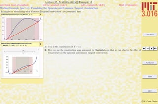
Worked Example (part A): Visualizing the Spinodal and Common Tangent Construction
notebook (non-evaluated) pdf (evaluated, color) pdf (evaluated, b&w) html (evaluated)
The spinodal and common tangent construction is a fundamental thermodynamic concept used for the creation of an alloy phase diagram
from molar-free energies. This construction appears repeatedly in studies of materials.
An example of visualizing this construction as a function of temperature will be worked out in detail for the case of a single curve and a
binary alloy.
First, we will work out all the steps in detail that are used to build up a single visualization, and then we will collect it all together in a
reusable function.
A prototype molar free energy of mixing using the same xlogx function for
the ideal entropy of mixing terms. The temperature term is a scaled
energy (RT), and it is assumed that enthalpies have been scaled so that
the temperatures of interest (if there are any) are between T=0 and T=10.
1
xlogx@0D =
xlogx@1D = xlogx@0.0D = xlogx@1.0D = 0;
xlogx@x_D := x Log@xD
Gmolar@X_, T_D :=
5 X H1 - XL + T Hxlogx@XD + xlogx@1 - XDL + X ê 2
Here is the shape of our prototype free energy at T=3/2
2p1 = Plot@Gmolar@x, 3 ê 2D,
8x, 0, 1<, PlotStyle Ø ThickD
We will need the bounds of the above graphics object:
3
88graphxmin, graphxmax<,
8graphymin, graphymax<< =
PlotRange ê. AbsoluteOptions@p1, PlotRangeD
First let's determine where the spinodal region (by finding where the
second derivative with respect to composition is negative
4ddg = D@Gmolar@x, 3 ê 2D, 8x, 2<D
Then, use RegionPlot to illustrate the range over which spinodal decompo-
sition is spontaneous
5
p2 = RegionPlot@ddg < 0,
8x, graphxmin, graphxmax<,
8T, graphymin, graphymax<,
PlotStyle Ø RGBColor@0, 1, .5, 0.1DD
Show them both together to identify the spinodal region
6Show@p1, p2D
1: We cook up a prototypical molar free-energy as a function of molar composition, X, and temperature
T. The x log x terms are calculated with a handy function, xlogx , which will handle the zeroes without
numerical difficulty at 0 Log[0].
2: The molar free-energy is plotted at a particular temperature (T = 1.5) and assigned to a symbol, pl.
3: We will need the bounds of the plot to create other graphical objects. We grab the bounds with
AbsoluteOptions and assign them to variables using a handy assignment construction {a,b} =
List.
4: The spinodal region is the easiest to visualize—it is the region where the second derivative of the
molar free-energy is negative. The second derivative is assigned to ddg.
5: RegionPlot evaluates its first argument over a square region and fills where the argument is true.
It is exactly what we need in order to visualize the spinodal region. We use the bounds that we
calculated from the free energy curve as the bounds for RegionPlot.
6: Showing both plots together, we visualize the spinodal region.

93. 3.016 Home
Full Screen
Close
Quit
c W. Craig Carter
Lecture 05 Mathematica R Example 15
Worked Example (part B): Visualizing the Spinodal and Common Tangent Construction
notebook (non-evaluated) pdf (evaluated, color) pdf (evaluated, b&w) html (evaluated)
The common tangent is any finite line segment that touches the molar free-energy at two points which have the same derivative. For
phase diagrams, we are interested only in lower common tangents (i.e., lines that touch the molar free-energy, but always lie below all
values). One can picture the common tangent by imagining that an elastic string is stretched along a molar free-energy curve; the common
tangents are where the string pulls away from the the curves.
The common tangent is related to the convex hull that appears in computational geometry.
We can use the ConvexHull to find the common tangent lines; this
function is in the Computational Geometry Package.
1<< ComputationalGeometry`
First we compute a list of values along the molar free energy curve, then
compute those that lie outside the common tangent(s) (i.e., the convex
hull). Because the points are given in order, we might as well
sort them on the way back out. Note, the convex hull program gives the
indices of the vertices that are on the hull.
2
npoints = 100;
gvals = Table@8x, Gmolar@x, 3 ê 2D<,
8x, 0, 1, 1 ê N@npoints - 1D<D;
We only want the lower convex hull; therefore we add some "fictive"
points to the beginning and the end of the data. The the fictive points
add a rectangle to the top of the curve that should be part of the com-
puted convex hull.
3
gmax = Max@Transpose@gvalsD@@2DDD;
PrependTo@gvals, 80, 10 * Abs@gmaxD<D;
AppendTo@gvals, 81, 10 * Abs@gmaxD<D;
After we compute this hull, we shift the hull by one and take off its first
and last element. We strip the first and last element from the discrete
values of free energy as well.
4
chull = Sort@ConvexHull@gvalsDD;
chull = Drop@Drop@chull - 1, 1D, -1D
gvals = Drop@Drop@gvals, 1D, -1D
The common tangent(s) correspond to gaps in the vertex list of the
common tangent. We will use Split to find the set of continous sequences.
5convexparts = Split@chull, HÒ2 - Ò1 < 2L &D
881, 2, 3, 4, 5, 6<, 895, 96, 97, 98, 99, 100<<
1: To calculate convex hulls, the ComputationalGeometry package is needed.
2: ConvexHull operates on discrete data. Discrete data are created by evaluating Gmolar at npoints
evenly-spaced mesh-points. We use Table and assign the discrete data list to gvals.
3: ConvexHull calculates the entire hull (i.e., the polygon that encloses all other points), and we are
only interested in the lower hull. Thus, we add a rectangle to the top of the data which is guaranteed
to be part of the hull, calculate the hull and discard the upper parts. Here we use PrependTo to add
a point ten times higher than the maximum value on the left side of the region, and use AppendTo
to add a corresponding point to the right side of the region. We have thus added a known rectangle
that we will remove later.
4: ConvexHull returns a list of indices of points from the original data. Because the original data was
created in an orderly left-to-right way, we can use Sort to put the data in a predictable form.
Because there was an additional point added at the beginning of gvals, we will need to shift the
indices down by one (by subtracting 1 from each index), and then we use Drop to remove the first
and last elements of both chull and gvals.
5: Thinking about the indices on the convex hull, any ordered sequence of the sorted list must be part
of original discrete data and also part of the convex hull. We are interested in connecting the last
point of any isolated sequence to the first point of the next sequence. We can use Split to find the
isolated sequences.

94. 3.016 Home
Full Screen
Close
Quit
c W. Craig Carter
Lecture 05 Mathematica R Example 16
Worked Example (part C): Visualizing the Spinodal and Common Tangent Construction
notebook (non-evaluated) pdf (evaluated, color) pdf (evaluated, b&w) html (evaluated)
With the information contained in the convex hull data, graphical objects are created to represent the gaps in that data. The gaps
coincide with the common tangents.
Now we create graphics objects for each of the two-phase regions (i.e.,
the gaps in the convex hull) and collect them all into a graphics list for
subsequent display.
1
len = Length@convexpartsD;
graphicslist = 8<;
i = 1;
While@i + 1 § len, leftpoint =
gvals@@Last@ convexparts@@iDD D DD ;
rightpoint = gvals@@
First@ convexparts@@i + 1DD D DD;
ctline = 8Red, Thick,
Line@8leftpoint, rightpoint<D<;
twophaseregion = 8RGBColor@0.5, 0, 0, 0.2D,
Rectangle@8leftpoint@@1DD, graphymin<,
8rightpoint@@1DD, graphymax<D<;
AppendTo@graphicslist, ctlineD;
AppendTo@graphicslist, twophaseregionD;
i++
D
p3 = Graphics@graphicslistD
2Show@p1, p2, p3D
1: We traverse the list convexparts and construct graphical objects corresponding to the regions of
isolated sequences. Because it is possible that a curve may have any number of common tangents,
we accumulate graphics primitives in a list as we encounter common tangents. A graphics object is
created from the list of graphics primitives.
The number of isolated sequences is assigned to len and we start with an empty list graphicslist.
Then, we loop over the list of length len. At each iteration in the loop, we identify the last vertex
on the previous point of the convex hull sequence and the first part of the next sequence. We use
those indices to extract the points on the curve that have been stored in gvals. With the two points,
we create red lines for the common tangents—and with the extra graphical information about the
original plot, draw a rectangle for the region.
Finally, a new graphics object (p3) is created.
2: Our final visualization is obtained by showing all three graphics objects together.

95. 3.016 Home
Full Screen
Close
Quit
c W. Craig Carter
Lecture 05 Mathematica R Example 17
Worked Example (part D): Visualizing the Spinodal and Common Tangent Construction
notebook (non-evaluated) pdf (evaluated, color) pdf (evaluated, b&w) html (evaluated)
The previous three parts illustrate how one might actually go about developing a complex visualization: create simple working
parts and then integrate them together into something more complex. (Don’t get the impression that I didn’t make any er-
rors or silly conceptual mistakes as I created this example! It was very time consuming and, while it looks fairly straightforward
in hindsight, it was a challenge to build.) However, once finished, it is useful to collect everything into a single function that can be reused.
1
Needs@"ComputationalGeometry`"D;
CommonTangentConstruction@
Gm_, T_, npts_: 100D :=
Module@8x, y, p1, p2, p3, gxmin, gxmax,
gymin, gymax, ddg, gvals, gmax,
chull, conprts, len, glist = 8<, i = 1,
lftpt, rtpt, ctline, twophasreg<,
p1 = Plot@Gm@x, TD, 8x, 0, 1<,
PlotStyle Ø ThickD;
88gxmin, gxmax<, 8gymin, gymax<< =
PlotRange ê.
AbsoluteOptions@p1, PlotRangeD;
ddg = D@Gm@x, TD, 8x, 2<D;
p2 = RegionPlot@ddg < 0,
8x, gxmin, gxmax<, 8y, gymin, gymax<,
PlotStyle Ø RGBColor@0, 1, .5, 0.1DD;
gvals = Table@8x, Gm@x, TD<,
8x, 0, 1, 1 ê N@npts - 1D<D;
gmax = Max@Transpose@gvalsD@@2DDD;
PrependTo@gvals, 80, 10 * Abs@gmaxD<D;
AppendTo@gvals, 81, 10 * Abs@gmaxD<D;
chull = Sort@ConvexHull@gvalsDD;
chull = Drop@Drop@chull - 1, 1D, -1D;
gvals = Drop@Drop@gvals, 1D, -1D;
conprts = Split@chull, HÒ2 - Ò1 < 2L &D;
len = Length@conprtsD;
While@i + 1 § len,
lftpt = gvals@@Last@ conprts@@iDD D DD ;
rtpt = gvals@@ First@ conprts@@i + 1DD D DD;
ctline =
8Red, Thick, Line@8lftpt, rtpt<D<;
twophasreg = 8RGBColor@0.5, 0, 0, 0.2D,
Rectangle@8lftpt@@1DD, gymin<,
8rtpt@@1DD, gymax<D<;
AppendTo@glist, ctlineD;
AppendTo@glist, twophasregD; i++D;
p3 = Graphics@glistD; Show@p1, p2, p3DD
1: Here is the result, CommonTangentConstruction , which collects the previous three examples together
and returns a single graphical object. CommonTangentConstruction takes two arguments for the
molar free-energy function, Gm, and temperature T, and an optional third argument for the precision
to calculate the hull. The optional argument is indicated by the :100 and will default to 100 if not
passed to the function.
The first argument must be the name of a defined function of composition and temperature.

96. 3.016 Home
Full Screen
Close
Quit
c W. Craig Carter
Lecture 05 Mathematica R Example 18
Worked Example (part E): Visualizing the Spinodal and Common Tangent Construction
notebook (non-evaluated) pdf (evaluated, color) pdf (evaluated, b&w) html (evaluated)
Examples of visualizing with CommonTangentConstruction are presented here.
1CommonTangentConstruction@Gmolar, 1.5D
2Manipulate@CommonTangentConstruction@
Gmolar, T, 300D, 88T, 2<, 0, 3<D
T
1: This is the construction at T = 1.5.
2: Here we use the construction as an argument to Manipulate so that we can observe the effect of
temperature on the spinodal and common tangent construction.

97. 3.016 Home
Full Screen
Close
Quit
c W. Craig Carter
Sept. 17 2007
Lecture 6: Linear Algebra I
Reading:
Kreyszig Sections: 7.5, 7.6, 7.7, 7.8, 7.9 (pages302–305, 306–307, 308–314, 315–323, 323–329)
Vectors
Vectors as a list of associated information
x =


number of steps to the east
number of steps to the north
number steps up vertical ladder

 (6-1)
x =


3
2.4
1.5

 determines position


xeast
xnorth
xup

 (6-2)
The vector above is just one example of a position vector. We could also use coordinate systems that differ from the Cartesian
(x, y, z) to represent the location. For example, the location in a cylindrical coordinate system could be written as
x =


x
y
z

 =


r cos θ
r sin θ
z

 (6-3)

98. 3.016 Home
Full Screen
Close
Quit
c W. Craig Carter
i.e., as a Cartesian vector in terms of the cylindrical coordinates (r, θ, z).
The position could also be written as a cylindrical, or polar vector
x =


r
θ
z

 =


x2 + y2
tan−1 y
x
z

 (6-4)
where the last term is the polar vector in terms of the Cartesian coordinates. Similar rules would apply for other coordinate
systems like spherical, elliptic, etc.
However, vectors need not represent position at all, for example:
n =










number of Hydrogen atoms
number of Helium atoms
number of Lithium atoms
...
number of Plutonium atoms
...










(6-5)
Scalar multiplication
1
Navag.
n ≡















number of H
Navag.
number of He
Navag.
number of Li
Navag.
...
number of Pu
Navag.
...















=










moles of H
moles of He
moles of Li
...
moles of Pu
...










= m (6-6)

99. 3.016 Home
Full Screen
Close
Quit
c W. Craig Carter
Vector norms
x ≡(x2
1 + x2
2 + . . . x2
k)1/2
= euclidean separation (also called l2-norm) (6-7)
n ≡nH + nHe + . . . n132? = total number of atoms (related to the Manhatten norm) (6-8)
Unit vectors
unit direction vector mole fraction composition (6-9)
ˆx =
x
x
ˆm =
m
m
(6-10)
Extra Information and Notes
Potentially interesting but currently unnecessary
If stands for the set of all real numbers (i.e., 0, −1.6, π/2, etc.), then we can use a
shorthand to specify the position vector, x ∈ N (e.g., each of the N entries in the vector
of length N must be a real number, or must be in the set of real numbers, x ∈ .)
For the unit (direction) vector: ˆx = {x ∈ 3 | x = 1} (i.e, the unit direction vector is the
set of all position vectors such that their length is unity—or, the unit direction vector is the
subset of all position vectors that lie on the unit sphere. x and ˆx have the same number of
entries, but compared to x, the number of independent entries in ˆx is smaller by one.
For the case of the composition vector, it is unphysical to have a negative number of atoms,
therefore the mole fraction vector n ∈ ( +)elements ( + is the real non-negative numbers)
and ˆm ∈ ( +)(elements-1).
Matrices and Matrix Operations
Consider methane (CH4), propane (C3H8), and butane (C4H10).

100. 3.016 Home
Full Screen
Close
Quit
c W. Craig Carter
MHC =
H-column C-column




number of H
methane molecule
number of C
methane molecule
number of H
propane molecule
number of C
propane molecule
number of H
butane molecule
number of C
butane molecule




methane row
propane row
butane row
(6-11)
MHC =


4 1
8 3
10 4

 =


M11 M12
M21 M22
M31 M32

 (6-12)
Matrices as a linear transformation of a vector
NHC = (number of methanes, number of propanes, number of butanes) (6-13)
= (NHC m, NHC p, NHC b) (6-14)
= (NHC 1, NHC 2, NHC 3) (6-15)
(6-16)
NHCMHC ≡
3
i=1
NHC iMHC ij = N (6-17)
The “summation” convention is often used, where a repeated index is summed over all its possible values:
p
i=1
NHC iMHC ij ≡ NHC iMHC ij = Nj (6-18)

101. 3.016 Home
Full Screen
Close
Quit
c W. Craig Carter
For example, suppose
NHC = (1.2 × 1012
molecules methane, 2.3 × 1013
molecules propane, 3.4 × 1014
molecules butane) (6-19)
NHCMHC =
(1.2 × 1014
methanes, 2.3 × 1013
propanes, 3.4 × 1012
butanes)




4 atoms H
methane
1 atoms C
methane
8 atoms H
propane
3 atoms C
propane
10 atoms H
butane
4 atoms C
butane




=(7.0 × 1014
atoms H, 2.0 × 1014
atoms C)
(6-20)
Matrix transpose operations
Above, the lists (or vectors) of atoms were stored as rows, but often it is convenient to store them as columns. The operation
to take a row to a column (and vice-versa) is called a “transpose”.
MHC
T
=
methane-column propane-column butane-column

number of H
methane molecule
number of H
propane molecule
number of H
butane molecule
number of C
methane molecule
number of C
propane molecule
number of C
butane molecule

 hydrogen row
carbon row
(6-21)
NHC
T
=


number of methanes
number of propanes
number of butanes

 =


NHC m
NHC p
NHC b

 (6-22)
MHC
T
NHC
T
= NT 4 8 10
1 3 4


number of methanes
number of propanes
number of butanes

 =
number of H-atoms
number of C-atoms
(6-23)

102. 3.016 Home
Full Screen
Close
Quit
c W. Craig Carter
Matrix Multiplication
The next example supposes that some process produces hydrocarbons and can be modeled with the pressure P and temperature
T. Suppose (this is an artificial example) that the number of hydrocarbons produced in one millisecond can be related linearly
to the pressure and temperature:
number of methanes = αP + βT
number of propanes = γP + δT
number of butanes = P + φT
(6-24)
or
NHC
T
=


α β
γ δ
φ

 P
T
(6-25)

103. 3.016 Home
Full Screen
Close
Quit
c W. Craig Carter
Lecture 06 Mathematica R Example 1
Matrices
notebook (non-evaluated) pdf (evaluated, color) pdf (evaluated, b&w) html (evaluated)
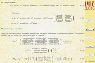
Here is an example operation that takes us from the processing vector (P, T)T
to the number of hydrogens and carbons.
MHC is our matrix that maps the three
hydrocarbons Hmethane CH4 , propane C3 H8 ,
butane C4 H10 , to number of hydrogens and carbons
1
MHC = 8
84, 1<,
88, 3<,
810, 4<
<
MHC êê MatrixForm
2Transpose@MHCD êê MatrixForm
PTmatrix is our matrix of kinetic data that
gives rates of change of a particular atomic species
HC or HL as a function of pressure and temperature
Hsee lecture notes corresponding to this Mathematica notebookL.
3
PTmatrix = 8
8a, b<,
8g, d<,
8e, f<
<;
PTmatrix êê MatrixForm
4MPT = MHC. PTmatrix
The matrix multiplication does not work
because the sizes are inconsistent.
5Clear@MPTD
6
MPT = Transpose@MHCD. PTmatrix;
MPT êê MatrixForm
1: The matrix (Eq. 6-12) is entered as a list of sublists. The sub-lists are the rows of the matrix. The
first elements of each row-sublist form the first column; the second elements are the second column
and so on.
The Length of a matrix-object gives the number of rows, and the second member of the result of
Dimensions gives the number of columns.
All sublists of a matrix must have the same dimensions.
It is good practice to enter a matrix and then display it separately using MatrixForm. Otherwise,
there is a risk of defining a symbol as a MatrixForm-object and not as a matrix which was probably
the intent.
2: The Transpose function exchanges the rows and columns. If Dimensions[Mat] returns {r,c}, then
Dimensions[Transpose[Mat]] returns {c,r}.
3: Dimensions[PTmatrix] is {3,2}.
4: This command will generate an error.
Matrix multiplication in Mathematica R is produced by the ”dot” ( . ) operator—and not the
”multiplication” ( * ) operator. For matrix multiplication, A.B, the number of columns of A must
be equal to the number of rows of B.
6: The Transpose “flips” a matrix by producing a new matrix which has the original’s ith
row as the
new matrix’s ith
column (or, equivalently the jth
column as the new jth
row). In this example, a
3 × 2-matrix (PTmatrix) is being left-multiplied by a a 2 × 3-matrix.
The resulting matrix would map a vector with values P and T to a vector for the rate of production
of C and H.

104. 3.016 Home
Full Screen
Close
Quit
c W. Craig Carter
Matrix multiplication is defined by:
AB =
i
AkiBij (6-26)
The indices of the matrix defined by the multiplication AB = C are Ckj.
Matrix Inversion
Sometimes what we wish to know is: “What vector is it (x), when transformed by some matrix (A), that gives us a particular
result (b = Ax)?”
Ax = b
A−1
Ax = A−1
b
x = A−1
b
(6-27)
The inverse of a matrix is defined as: something, that when multiplied with the matrix, leaves a product that has no effect
on any vector. This special product matrix is called the identity matrix.

105. 3.016 Home
Full Screen
Close
Quit
c W. Craig Carter
Lecture 06 Mathematica R Example 2
Inverting Matrices
notebook (non-evaluated) pdf (evaluated, color) pdf (evaluated, b&w) html (evaluated)
Our last example produced a linear operation that answered the question, “given a particular P and T, at what rate will C and H be
produced?”
To answer the converse question, “If I want a particular rate of production for C and H, at what P and T should the process be carried
out?”
To invert the question on linear processes, the matrix is inverted.
1
MPT = Transpose@MHCD. PTmatrix;
MPTinverse = Factor@Inverse@MPTDD;
MPTinverse êê MatrixForm
- b+3 d+4 f
2 H2 b g-2 a d+3 b e+d e-3 a f-g fL
2 b+4 d+5 f
2 b g-2 a d+3 b e+d e-3 a f-g f
-
a+3 g+4 e
2 H-2 b g+2 a d-3 b e-d e+3 a f+g fL
2 a+4 g+5 e
-2 b g+2 a d-3 b e-d e+3 a f+g f
The denominators are related to the determinant---if the determinant
vanishes, then the inverse matrix is not defined.
2Det@MPTD
Checking to see if the the inverse multiplied by the original matrix is the
identity matrix:
3MPT.MPTinverse
It is not obvious unless simplified...
4Simplify@MPT.MPTinverseD êê MatrixForm
K
1 0
0 1
O
1: Inverting a matrix by hand is tedious and prone to error, Inverse does this in Mathematica R
. In this example, Factor is called on the result of Inverse. Factor is an example of a threadable
function—it recursively operates on all members of any argument that is a list-object. Thus, each
of the entries in the inverted matrix is factored individually.
2: The determinant of a matrix is fundamentally linked to the existence of its inverse. In this example,
it is observed that if the Det of a matrix vanishes, then the entries of its inverse are undetermined.
3: The multiplication of a matrix by its inverse should produce the identity matrix (i.e., a matrix with
1 at each diagonal entry, and zero otherwise). That this multiplication gives the identity matrix is
not obvious. Unless, . . .
4: Simplify is called on each of the entries.

106. 3.016 Home
Full Screen
Close
Quit
c W. Craig Carter
Linear Independence: When solutions exist
Ax = b
a11 a12
a21 a22
x
y
=
b1
b2
(6-28)
a11x+a12y =b1
a11x+a12y =b1
a11x+a12y =b1
a21x+a22y =b2
a21x+a22y =b2a21x+a22y =b2
b1
a12
b2
a22
No Solution One Unique Solution Infinitely Many Solutions
Figure 6-1: Geometric interpretation of solutions in two dimensions

107. 3.016 Home
Full Screen
Close
Quit
c W. Craig Carter
Lecture 06 Mathematica R Example 3
Eliminating redundant equations or variables
notebook (non-evaluated) pdf (evaluated, color) pdf (evaluated, b&w) html (evaluated)
Consider liquid water near the freezing point—dipole interactions will tend to make water molecules form clusters such as H2O and H4O2.
This example looks at such a case where the columns are not linearly independent.
Same example for water and water complexes: use the matrix watmat to
store molecular formulas for each type of molecule in the system
1watmat = 882, 4<, 81, 2<<;
watmat êê MatrixForm
The vector molvec is used to store the number of each kind of molecule
2molvec = 8h20, h402<
The vector atomvec is used to store the number of each atomic species
that is present
3atomvec = 8h, o<
4atomvec êê MatrixForm
The vector eq is now defined and its two elements are equations that
give the number of hydrogen atoms and the number of oxygen atoms:
5eq@1D = Hwatmat.molvecL@@1DD ä atomvec@@1DD
6eq@2D = Hwatmat.molvecL@@2DD ä atomvec@@2DD
7Solve@8eq@1D, eq@2D<, molvecD
8? Eliminate
Eliminate@eqns, varsD eliminates
variables between a set of simultaneous à
9Eliminate@8eq@1D, eq@2D<, molvecD
2 o ã h
10MatrixRank@watmatD
11NullSpace@watmatD
Length@NullSpace@watmatDD
88-2, 1<<
1: The mapping from molecules to the number of atoms becomes:
„
2 4
1 2
« „
NH2O
NH4O2
«
=
„
NH
NO
«
(6-29)
The matrix watmat encodes the coefficients in these linear equations.
2–5: The vectors, atomvec and molvec, represent the numbers of each type of atom and each type of
molecule.
5–6: These equations are the same as the rows of Ax being set to the corresponding entry of b for Ax = b.
These are the linear equations given above.
7: This is an attempt (using Solve on the linear equations) to find the number of H2O- and H4O2-
molecules, given the number of H- and O-atoms. Of course, it has to fail.
8–9: Eliminate produces a logical equality for each redundancy in a set of equations. In this case, the
result expresses the fact that 2 × (second row) is the same as the (first row).
10: The rank of a matrix, obtained with MatrixRank, gives the number of linearly independent rows.
11: The null space of a matrix, A, is a linearly independent set of vectors x, such that Ax is the zero-
vector; this list can be obtained with NullSpace. The result is equivalent to that obtained with
Eliminate in item 9. The nullity is the number of vectors in a matrix’s null space. The rank and
the nullity must add up to the number of columns of A

108. 3.016 Home
Full Screen
Close
Quit
c W. Craig Carter
Sept. 19 2007
Lecture 7: Linear Algebra
Reading:
Kreyszig Sections: 13.1, 13.2, 13.5, 13.6 (pages602–606, 607–611, 623–626, 626–629)
Uniqueness and Existence of Linear System Solutions
It would be useful to use the Mathematica Help Browser and open the link to Matrices & Linear Algebra in
the Mathematics & Algorithms section. Look through the tutorials at the bottom on the linked page.
A linear system of m equations in n variables (x1, x2, . . . , xn) takes the form
A11x1 + A12x2 + A13x3 + . . . + A1nxn = b1
A21x1 + A22x2 + A23x3 + . . . + A2nxn = b2
... =
...
Ak1x1 + Ak2x2 + Ak3x3 + . . . + Aknxn = bk
... =
...
Am1x1 + Am2x2 + Am3x3 + . . . + Amnxn = bm
(7-1)
and is fundamental to models of many systems.
The coefficients, Aij, form a matrix and such equations are often written in an “index” short-hand known as the Einstein
summation convention:
Ajixi = bj (Einstein summation convention) (7-2)

109. 3.016 Home
Full Screen
Close
Quit
c W. Craig Carter
where if an index (here i) is repeated in any set of multiplied terms, (here Ajixi) then a summation over all values of that
index is implied. Note that, by multiplying and summing in Eq. 7-2, the repeated index i disappears from the right-hand-side.
It can be said that the repeated index in “contracted” out of the equation and this idea is emphasized by writing Eq. 7-2 as
xiAji = bj (Einstein summation convention) (7-3)
so that the “touching” index, i, is contracted out leaving a matching j-index on each side. In each case, Eqs. 7-2 and 7-3
represent m equations (j = 1, 2, . . . , m) in the n variables (i = 1, 2, . . . , n) that are contracted out in each equation. The
summation convention is especially useful when the dimensions of the coefficient matrix is larger than two; for a linear elastic
material, the elastic energy density can be written as:
Eelast =
1
2
ijCijkl kl =
1
2
σpqSpqrsσrs (7-4)
where Cijkl and ij are the fourth-rank stiffness tensor and second-rank elastic strain tensor; where Sijkl and σij are the
fourth-rank compliance tensor and second-rank stress tensor;
In physical problems, the goal is typically to find the n xi for a given m bj in Eqs. 7-2, 7-3, or 7-1. This goal is conveniently
represented in matrix-vector notation:
Ax = b (7-5)

110. 3.016 Home
Full Screen
Close
Quit
c W. Craig Carter
Lecture 07 Mathematica R Example 1
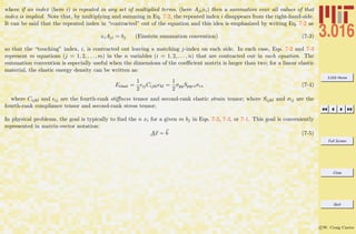
Solving Linear Sets of Equations
notebook (non-evaluated) pdf (evaluated, color) pdf (evaluated, b&w) html (evaluated)
Demonstrations of several different ways to solve a set of linear equations for several variables. Here we will solve equations that we
construct from matrices; in following examples, we will operate on the matrices directly.
Consider the set of equations
x + 2y + z + t = a
-x + 4y - 2z = b
x + 3y + 4z + 5t = c
x + z + t = d
We illustrate how to use a matrix representation to write these out and
solve them…
Start with the matrix of coefficients of the variables, mymatrix:
1
mymatrix = 8
81, 2, 1, 1<,
8-1, 4, -2, 0<,
81, 3, 4, 5<,
81, 0, 1, 1<<;
mymatrix êê MatrixForm
The system of equations will only have a unique solution if the determi-
nant of mymatrix is nonzero.
2Det@mymatrixD
Now define vectors for x and b
”
in Aê x = b
”
3myx = 8x, y, z, t<;
4myb = 8a, b, c, d<;
The left-hand side of the first equation will be
5Hmymatrix.myxL@@1DD
and the left-hand side of all four equations will be
6lhs = mymatrix.myx;
lhs êê MatrixForm
Now define an indexed variable linsys with four entries, each being one
of the equations in the system of interest:
7linsys@i_IntegerD := lhs@@iDD == myb@@iDD
8linsys@2D
Solving the set of equations for the unknowns x
Ø
9linsol = Solve@8linsys@1D,
linsys@2D, linsys@3D, linsys@4D<, myxD
1: This example is kind of backwards. We will take a matrix
A =
0
B
B
@
1 2 1 1
−1 4 −2 0
1 2 4 5
1 0 1 1
1
C
C
A unknown vector x =
0
B
B
@
x
y
z
t
1
C
C
A and known vector b =
0
B
B
@
a
b
c
d
1
C
C
A
and extract four equations for input to Solve to obtain the solution to x. Here, the coefficient
matrix is a list of row-lists.
2: A unique solution will exist if the determinant, computed with Det, is non-zero.
3–4: These will be the left-hand- and right-hand-side vectors.
5: Matrix multiplication is indicated by the period ( .). This will be the first of the equations.
6: lhs is a column-vector with four entries, and each entry is one of the lhs equations.
7–8: This function creates logical equalities for each corresponding entry on the left- and right-hand-sides.
unknowns.
9: The function Solve is used on a system of equations ({linsys[i]} and variables.

111. 3.016 Home
Full Screen
Close
Quit
c W. Craig Carter
Lecture 07 Mathematica R Example 2
Inverting Matrices or Just Solving for the Unknown Vector
notebook (non-evaluated) pdf (evaluated, color) pdf (evaluated, b&w) html (evaluated)
Continuing the last example, it is much more compact to invert a matrix symbolically or numerically. If a matrix inverse is going to be
used over and over again, it is probably best to compute and store the inverse once. However, if a one-time only solution for x in Ax = b
is needed, then computing the inverse is computationally less efficient than using an algorithm designed to solve for x directly. Here is
an example of both methods.
Doing the same thing a different way, using Mathematica's LinearSolve
function:
1? LinearSolve
LinearSolve@m, bD finds an x which solves the
LinearSolve@mD generates a LinearSolveFunction
which can be applied repeatedly to different à
2LinearSolve@mymatrix, mybD
And yet another way, based on x = A
-1
A x = A
-1
b
3Inverse@mymatrixD.myb êê MatrixForm
a
7
+ b
7
- 2 c
7
+ 9 d
7
a
2
- d
2
13 a
14
- 4 b
7
+ c
7
- 23 d
14
- 15 a
14
+ 3 b
7
+ c
7
+ 19 d
14
And yet even another way, a very efficient LinearSolveFunction can be
produced by LinearSolve. This function will operate on any rhs vector of
the appropriate length. This would be an efficient way to find the numeri-
cal solution to a known matrix, but for many different rhs b.
4mymatrixsol = LinearSolve@mymatrixD;
The result can be applied as a function calling a vector :
5mymatrixsol@mybD
Simplify@mymatrixsol@mybDD
:
1
7
Ha + b - 2 c + 9 dL,
a - d
2
,
1
14
H13 a - 8 b + 2 c - 23 dL,
1
14
H-15 a + 6 b + 2 c + 19 dL>
1–2: LinearSolve can take two arguments, A and b, and returns x that solves Ax = b. It will be noticibly
faster than the following inversion method, especially for large matrices.
3: The matrix inverse is obtained with Inverse and a subsequent multiplication by the right-hand-side
gives the solution.
4–5: Calling LinearSolve on a matrix alone, returns an efficient function that takes the unknown vector
as an argument. Here we show the equivalence to item 3.

112. 3.016 Home
Full Screen
Close
Quit
c W. Craig Carter
Uniqueness of solutions to the nonhomogeneous system
Ax = b (7-6)
Uniqueness of solutions to the homogeneous system
Axo = 0 (7-7)
Adding solutions from the nonhomogeneous and homogenous systems
You can add any solution to the homogeneous equation (if they exist, there are infinitely many of them) to any solution to
the nonhomogeneous equation, and the result is still a solution to the nonhomogeneous equation.
A(x + xo) = b (7-8)
Determinants

113. 3.016 Home
Full Screen
Close
Quit
c W. Craig Carter
Lecture 07 Mathematica R Example 3
Determinants, Rank, and Nullity
notebook (non-evaluated) pdf (evaluated, color) pdf (evaluated, b&w) html (evaluated)
Several examples of determinant calculations are provided to illustrate the properties of determinants. When a determinant vanishes
(i.e., det A = 0), there is no solution to the inhomogeneous equation det A = b, but there will be an infinity of solutions to det A = 0; the
infinity of solutions can be characterized by solving for a number rank of the entries of x in terms of the nullity of other entries of x
Create a matrix with one row as a linear combination of the others
1
myzeromatrix =
8mymatrix@@1DD, mymatrix@@2DD,
p * mymatrix@@1DD +
q * mymatrix@@2DD + r * mymatrix@@4DD,
mymatrix@@4DD<;
myzeromatrix êê MatrixForm
1 2 1 1
-1 4 -2 0
p - q + r 2 p + 4 q p - 2 q + r p + r
1 0 1 1
2Det@myzeromatrixD
3LinearSolve@myzeromatrix, mybD
This was not expected to have a solution
4MatrixRank@mymatrixD
MatrixRank@myzeromatrixD
5NullSpace@mymatrixD
NullSpace@myzeromatrixD
Try solving this inhomogeneous system of equations using Solve:
6zerolhs = myzeromatrix.myx
7
zerolinsys@i_IntegerD :=
zerolhs@@iDD == myb@@iDD
8zerolinsolhet =
Solve@Table@zerolinsys@iD, 8i, 4<D, myxD
No solution, as expected, Let's solve the homogeneous problem:
9zerolinsolhom = Solve@Table@zerolinsys@iD ê.
8a Ø 0, b Ø 0, c Ø 0, d Ø 0<, 8i, 4<D, myxD
88y Ø 0, x Ø -2 t, z Ø t<<
1: A matrix is created where the third row is the sum of p×first row, q×second row, and r×fourth row.
In other words, one row is a linear combination of the others.
2: The determinant is computed with Det, and its value should reflect that the rows are not linearly
independent.
3: An attempt to solve the linear inhomogeneous equation (here, using LinearSolve) should fail.
4: When the determinant is zero, there may still be some linearly-independent rows or columns. The
rank gives the number of linearly-independent rows or columns and is computed with MatrixRank.
Here, we compare the rank of the original matrix and the linearly-dependent one we created.
5: The null space of a matrix, A, is a set of linearly-independent vectors that, if left-multiplied by A,
gives a zero vector. The nullity is how many linearly-independent vectors there are in the null space.
Sometimes, vectors in the null space are called killing vectors. By comparing to the above, you will
see examples of the rank + nullity = dimension rule for square matrices.
6–8: Here, an attempt to use Solve for the heterogeneous system with vanishing determinant is at-
tempted, but of course it is bound to fail. . .
9: However, this is the solution to the singular homogeneous problem (Ax = 0, where det A = 0. The
solution is three (the rank) dimensional surface embedded in four dimensions (the rank plus the
nullity). Notice that the solution is a multiple of the null space that we computed in item 5.

114. 3.016 Home
Full Screen
Close
Quit
c W. Craig Carter
Properties and Roles of the Matrix Determinant
In example 07-1, it was stated (item 2) that a unique solution exists if the matrix’s determinant was non-zero. The solution,
x =





2a+2b−4c+18d
det A
7a−7d
det A
13a−8b+2c−23d
det A
−15a+6b+2c+19d
det A





(7-9)
indicates why this is the case and also illustrates the role that the determinant plays in the solution. Clearly, if the determinant
vanishes, then the solution is undetermined unless b is a zero-vector 0 = (0, 0, 0, 0). Considering the algebraic equation, ax = b,
the determinant plays the same role for matrices that the condition a = 0 plays for algebra: the inverse exists when a = 0 or
det A = 0.
The determinant is only defined for square matrices; it derives from the elimination of the n unknown entries in x using all
n equation (or rows) of
Ax = 0 (7-10)
For example, eliminating x and y from
a11 a12
a21 a22
x
y
=
0
0
gives the expression
det
a11 a12
a21 a22
≡ a11a22 − a12a21 = 0
(7-11)
and eliminating x, y, and z from


a11 a12 a13
a21 a22 a23
a31 a32 a33




x
y
z

 =


0
0
0


gives the expression
detA ≡ a11a22a33 − a11a32a23 + a21a32a13 − a21a12a33 + a31a12a23 − a31a22a13 = 0
(7-12)
The following general and true statements about determinants are plausible given the above expressions:

115. 3.016 Home
Full Screen
Close
Quit
c W. Craig Carter
• Each term in the determinant’s sum us products of N terms—a term comes from each column.
• Each term is one of all possible the products of an entry from each column.
• There is a plus or minus in front each term in the sum, (−1)p, where p is the number of neighbor exchanges required to
put the rows in order in each term written as an ordered product of their columns (as in Eqs. 7-11 and 7-12).
These, and the observation that it is impossible to eliminate x in Eqs. 7-11 and 7-12 if the information in the rows is
redundant (i.e., there is not enough information—or independent equations—to solve for the x), yield the general properties
of determinants that are illustrated in the following example.

116. 3.016 Home
Full Screen
Close
Quit
c W. Craig Carter
Lecture 07 Mathematica R Example 4
Properties of Determinants and Numerical Approximations to Zero
notebook (non-evaluated) pdf (evaluated, color) pdf (evaluated, b&w) html (evaluated)
Rules, corresponding to how det A changes when the columns of A are permuted or multiplied by a constant, are demonstrated.
1
rv@i_D :=
rv@iD = Table@RandomReal@8-1, 1<D, 8j, 6<D
Now use rv to make a 6 x 6 matrix, then find its determinant:
2RandMat = Table@rv@iD, 8i, 6<D
3Det@RandMatD
Switching two rows changes the sign but not the magnitude of the
determinant:
4Det@8rv@2D, rv@1D, rv@3D, rv@4D, rv@5D, rv@6D<D
Multiply one row by a constant and calculate determinant:
5Det@8a * rv@2D, rv@1D,
rv@3D, rv@4D, rv@5D, rv@6D<D
Multiply two rows by a constant and calculate determinant:
6Det@8a * rv@2D, a * rv@1D,
rv@3D, rv@4D, rv@5D, rv@6D<D
Multiply all rows by a constant and calculate determinant:
7Det@
a 8rv@2D, rv@1D, rv@3D, rv@4D, rv@5D, rv@6D<D
8
Clear@a, b, c, d, eD
LinDepVec = a * rv@1D + b * rv@2D +
c * rv@3D + d * rv@4D + e * rv@5D
Example of numerical precision: this determinant should evaluate to
zero…
9Det@8rv@1D, rv@2D,
rv@3D, rv@4D, rv@5D, LinDepVec<D
-4.85723 µ 10-17
a + 4.85723 µ 10-17
b +
4.16334 µ 10-17
c - 4.85723 µ 10-17
d - 1.38778 µ 10-17
e
However, numerical precision does
10Chop@Det@8rv@1D, rv@2D,
rv@3D, rv@4D, rv@5D, LinDepVec<DD
1–2: A matrix, RandMat , is created from rows with random real entries between -1 and 1.
3–4: This will demonstrate that switching neighboring rows of a matrix changes the sign of the determi-
nant.
5–6: Multiplying one column of a matrix by a constant a, multiplies the matrix’s determinant by one
factor of a; multiplying two rows by a gives a factor of a2
. Multiplying every entry in the matrix by
a changes its determinant by an
.
7: Because the matrix has one linearly-dependent column, its determinant should vanish. This exam-
ple demonstrates what happens with limited numerical precision operations on real numbers. The
determinant is not zero, but could be considered effectively zero.
8: We create a row which is an arbitrary linear combination of the first five rows of RandMat.
9: This determinant should be zero. However, because the entries are numerical, differences which
are smaller than the precision with which a number is stored, may make it difficult to distinguish
between something that is numerically zero and one that is precisely zero. This is sometimes known
as round-off error.
10: Problems with numerical imprecision can usually be alleviated with Chop which sets small magnitude
numbers to zero.

117. 3.016 Home
Full Screen
Close
Quit
c W. Craig Carter
Lecture 07 Mathematica R Example 5
Determinants and the Order of Matrix Multiplication
notebook (non-evaluated) pdf (evaluated, color) pdf (evaluated, b&w) html (evaluated)
Symbolic matrices are constructed to show examples of the rules det(AB) = det A det B and AB = BA.
Creating a symbolic matrix
1SymVec = 8a, a, a, c, c, c<;
2Permuts = Permutations@SymVecD
Permuts êê Dimensions
3
SymbMat = 8
Permuts@@1DD,
Permuts@@12DD,
Permuts@@6DD,
Permuts@@18DD,
Permuts@@17DD,
Permuts@@9DD<;
SymbMat êê MatrixForm
4DetSymbMat = Simplify@Det@SymbMatDD
Creating a matrix of random rational numbers
5
RandomMat =
TableBTableB
RandomInteger@8-100, 100<D
RandomInteger@81, 100<D
,
8i, 6<F, 8j, 6<F;
MatrixForm@RandomMatD
6DetRandomMat = Det@RandomMatD
7CheckA = Det@SymbMat.RandomMatD êê Simplify
8DetRandomMat * DetSymbMat == CheckA
Does the determinant of a product depend on the order of multiplication?
9CheckB = Det@RandomMat.SymbMatD êê Simplify
10CheckA ã CheckB
However, the product of two matrices depends on which matrix is on the
left and which is on the right
11HRandomMat.SymbMat - SymbMat.RandomMatL êê
Simplify êê MatrixForm
1–3: Using Permutations to create all possible permutations of two sets of three identical objects for
subsequent construction of a symbolic matrix, SymbMat, for demonstration purposes.
4: The symbolic matrix has a fairly simple determinant—it can only depend on two symbols and must
be sixth-order.
5: A matrix with random rational numbers is created. . .
6: And, of course, its determinant is also a rational number.
7–10: This demonstrates that the determinant of a product is the product of determinants and is inde-
pendent of the order of multiplication. . .
11: However, the result of multiplying two matrices does depend on the order of multiplication: AB =
BA, in general.
Matrix multiplication is non-commutative: AB = BA for most matrices. However, any two matrices
for which the order of multiplication does not matter (AB = BA) are said to commute. Commutation
is an important concept in quantum mechanics and crystallography.
Think about what commuting matrices means physically. If two linear transformations commute,
then the order in which they are applied doesn’t matter. In quantum mechanics, an operation is
roughly equivalent to making an observation—commuting operators means that one measurement
does not interfere with a commuting measurement. In crystallography, operations are associated
with symmetry operations—if two symmetry operations commute, they are, in a sense, “orthogonal
operations.”

118. 3.016 Home
Full Screen
Close
Quit
c W. Craig Carter
The properties of determinants
Vector Spaces
Consider the position vector
x =


x
y
z

 =


x1
x2
x3

 (7-13)
The vectors (1, 0, 0), (0, 1, 0), and (0, 0, 1) can be used to generate any general position by suitable scalar multiplication and
vector addition:
x =


x
y
z

 = x


1
0
0

 + y


0
1
0

 + z


0
0
1

 (7-14)
Thus, three dimensional real space is “spanned” by the three vectors: (1, 0, 0), (0, 1, 0), and (0, 0, 1). These three vectors are
candidates as “basis vectors for 3.”
Consider the vectors (a, −a, 0), (a, a, 0), and (0, a, a) for real a = 0.
x =


x
y
z

 =
x + y
2a


a
−a
0

 +
x − y
2a


a
a
0

 +
x − y + 2z
2a


0
a
a

 (7-15)
So (a, −a, 0), (a, a, 0), and (0, a, a) for real a = 0 also are basis vectors and can be used to span 3.
The idea of basis vectors and vector spaces comes up frequently in the mathematics of materials science. They can represent
abstract concepts as well as being shown by the following two dimensional basis set:

119. 3.016 Home
Full Screen
Close
Quit
c W. Craig Carter
basis vector 1 basis vector 2
+ +
+ +
+ +
= =
= =
= =
1.0 1.0
0.5 0.7
0.2 1.0
1.0 0.1
1.0 0.5
1.0 0.0
Figure 7-2: A vector space for two-dimensional CsCl structures. Any combination of center-site
concentration and corner-site concentration can be represented by the sum of two basis vectors
(or basis lattice). The set of all grey-grey patterns is a vector space of patterns.
Linear Transformations

120. 3.016 Home
Full Screen
Close
Quit
c W. Craig Carter
Lecture 07 Mathematica R Example 6
Visualization Example: Polyhedra
notebook (non-evaluated) pdf (evaluated, color) pdf (evaluated, b&w) html (evaluated)
A simple octagon with different colored faces is transformed by operating on all of its vertices with a matrix. This example demonstrates
how symmetry operations, like rotations reflections, can be represented as a matrix multiplication, and how to visualize the results of
linear transformations generally.
We now demonstrate the use of matrix multiplication for manipulating an
object, specifically an octohedron. The Octahedron is made up of eight
polygons and the initial coordinates of the vertices were set to make a
regular octahedron with its main diagonals parallel to axes x,y,z. The
faces of the octahedron are colored so that rotations and other transforma-
tions can be easily tracked.
1<< "PolyhedronOperations`"
Show@PolyhedronData@"Octahedron"DD
Above, the color of the three dimensional object derives from the colors
in the light sources. For example, note that there appears to be a blue
light pointing down from the left. The lights stay fixed as we rotate the
object. If Lighting Ø None, then the polyhedron's faces will appear to be
black.
2Show@PolyhedronData@"Octahedron"D,
Lighting Ø NoneD
We can extract data from the Octahedron, and build our own with
individually colored faces. We will need the individual colors to identify
what happens to the polyhedron under linear transformaions.
3PolyhedronData@"Octahedron", "Faces"D
The object ColOct is defined below to draw an octahedron and it invokes
the Polygon function to draw the triangular faces by connecting three
points at specific numerical coordinates that we obtain from the Octahe-
dron data. Because we will turn off lighting, we will ask that each of the
faces glow, using the Glow graphics directive
4
octa = 8p@1D, p@2D, p@3D, p@4D, p@5D, p@6D< =
PolyhedronData@
"Octahedron", "Faces"D@@1DD;
colface@i_D := Glow@Hue@i ê 8DD ;
ColOct =
88colface@0D, Polygon@8p@4D, p@5D, p@6D<D<,
8colface@1D, Polygon@8p@4D, p@6D, p@2D<D<,
8colface@2D, Polygon@8p@4D, p@2D, p@1D<D<,
8colface@3D, Polygon@8p@4D, p@1D, p@5D<D<,
8colface@4D, Polygon@8p@5D, p@1D, p@3D<D<,
8colface@5D, Polygon@8p@5D, p@3D, p@6D<D<,
8colface@6D, Polygon@8p@3D, p@1D, p@2D<D<,
8colface@7D, Polygon@8p@6D, p@3D, p@2D<D<<;
5Show@Graphics3D@ColOctD, Lighting Ø NoneD
1: The package PolyhedronOperations contains Graphics Objects and other information such as
vertex coordinates of many common polyhedra. This demonstrates how an Octahedron can be
drawn on the screen. The color of the faces comes from the light sources. For example, there is a
blue source behind your left shoulder; as you rotate the object the faces—oriented so that they reflect
light from the blue source—will appear blue-ish. The color model and appearance is an advanced
topic.
2: Setting Lighting→None removes the light sources and the octahedron will appear black. Our
objective is to observe the effect of linear transformation on this object. To do this, will will want
to identify each of the octahedron’s faces by “painting” it.
3: We will build a custom octahedron from the Mm’s version using PolyhedronData.
4: The data is extracted by grabbing the first part of PolyhedronData (i.e., [[1]]). We assign the
name of the list octa , and name its elements p[i] in one step.
A function is defined and will be used to call Glow and Hue for each face. When the face glows and
the lighting is off, the face will appear as the “glow color”, independent of its orientation.
ColOct is a list of graphics-primitive lists: each element of the list uses the glow directive and then
uses the points of the original octahedron to define Polygons in three dimensions.
5: We wrap ColOct inside Graphics3D and use Show with lighting off to visualize.

121. 3.016 Home
Full Screen
Close
Quit
c W. Craig Carter
Lecture 07 Mathematica R Example 7
Linear Transformations: Matrix Operations on Polyhedra
notebook (non-evaluated) pdf (evaluated, color) pdf (evaluated, b&w) html (evaluated)
A moderately sophisticated Mathematica R function is defined to help visualize the effect of operating on each point of a polyhedron
with a 3 × 3-matrix representing a symmetry operation.
1
transoct@tmat_, description_StringD :=
8ColOct ê.
8Polygon@8a_List, b_List, c_List<D Ø
Polygon@8tmat.a, tmat.b, tmat.c<D<,
Text@Style@MatrixForm@tmatDD, 80, 0, -.25<D,
Text@Style@description, Darker@RedDD,
80, 0, .25<, Background Ø WhiteD<
2
Show@Graphics3D@
transoct@881, 0, 0<, 80, 1, 0<, 80, 0, -1<<,
"mirror-@001D"DD, Lighting Ø NoneD
3
identity = IdentityMatrix@3D;
rot90@001D = 880, -1, 0<, 81, 0, 0<, 80, 0, 1<<;
ref@010D = 881, 0, 0<, 80, -1, 0<, 80, 0, 1<<;
o@1, 1D = transoct@identity, "original"D;
o@1, 2D = transoct@rot90@001D, "90-@001D"D;
o@1, 3D = transoct@ref@010D, "m-@010D"D;
o@2, 1D = transoct@ref@010D.rot90@001D,
"90-@100D then m-@010D"D;
o@2, 2D = transoct@rot90@001D.ref@010D,
"m-@010D then 90-@100D"D;
4RotationTransform@Pi, 81, 1, 0<D
5o@2, 3D = transoctB
0 1 0
1 0 0
0 0 -1
, "180-@110D"F;
6
sc@q_, f_D :=
3 8Cos@qD Sin@fD, Sin@qD Sin@fD, Cos@fD<
Manipulate@GraphicsGrid@
Table@Show@Graphics3D@o@i, jDD,
Lighting Ø None, ViewPoint Ø sc@q, fD,
ImageSize Ø 8200, 200<,
PlotRange Ø 88-1, 1<, 8-1, 1<, 8-1, 1<<D,
8j, 3<, 8i, 2<DD, 88q, 2.1<, 0, 2 p<,
88f, -1.4<, -p ê 2, p ê 2<D
1: This is a moderately sophisticated example of rule usage inside of a function (transoct ) definition:
the pattern matches triangles ( Polygons with three points) in a graphics primitive; names the points;
and then multiplies a matrix by each of the points. The first argument to transoct is the matrix
which will operate on the points; the second argument is an identifyer that will be used with Text
to annonate the graphics.
2: This demonstrates the use of transoct : we get a rotate-able 3D object with floating text identifying
the name of the operation and the matrix that performs the operation.
3: We will build an example that will visualize several symmetry steps simultaneously (say that fast
outloud). We define matrices for identity , rot90[001] , and ref[010] , respectively, which leave the
polyhedra’s points unchanged, rotate counter-clockwise by 90◦
around the [001]-axis, and reflect
through the origin in the direction of the [010]-axis.
We use these matrices to create new octahedra corresponding to combinations of symmetry opera-
tions.
4–5: It is not always straightforward to write down the matrix corresponding to an arbitrary sym-
metry operation. Mathematica R has functions to help find many of them; here, we use
RotationTransform to find the matrix corresponding to rotation by 180◦
around the [110]-axis.
6: This will display six of the octahedra with their annotated symmetry operations. Manipulate is
used to change the viewpoint to someplace on a sphere of radius 3 (by changing the latitude angle,
φ, and the longitude θ). A function to return a cartesian representation of the spherical coordinates
is defined first and is used as the ViewPoint for each Graphics3D-object. Table iterates over the
o[i,j] and passes its result to GraphicsGrid.

122. 3.016 Home
Full Screen
Close
Quit
c W. Craig Carter
Lecture 07 Mathematica R Example 8
Visualization Example: Invariant Symmetry Operations on Crystals
notebook (non-evaluated) pdf (evaluated, color) pdf (evaluated, b&w) html (evaluated)
Each crystal’s unit cell can be uniquely characterized by the symmetry operations (i.e., fixed rotation about an axis, reflection across
a plane, and inversion through the origin) which leave the unit cell unchanged. The set of such symmetry operations define the crys-
tal point group. There are only 32 point groups in three dimensions. In this example, we demonstrate invariant operations for an FCC cell.
1
corners = Flatten@Table@8i, j, k<,
8i, 0, 1<, 8j, 0, 1<, 8k, 0, 1<D, 2D
faces = Join@Permutations@80.5, 0.5, 0<D,
Permutations@80.5, 0.5, 1<DD
fccsites = Join@faces, cornersD
srad = 2 í 4;
FCC = Table@
Sphere@fccsites@@iDD, sradD, 8i, 1, 14<D
axes = 8 8RGBColor@1, 0, 0, .5D,
Cylinder@880, 0, 0<, 82, 0, 0<<, .05D<,
8RGBColor@0, 1, 0, .5D,
Cylinder@880, 0, 0<, 80, 2, 0<<, .05D<,
8RGBColor@0, 0, 1, .5D,
Cylinder@880, 0, 0<, 80, 0, 2<<, .05D<<;
fccmodel = Translate@Join@FCC, axesD,
8-.5, -.5, -.5<D
Graphics3D@fccmodelD
2
bbox = 1.25 88-1, 1<, 8-1, 1<, 8-1, 1<<;
ManipulateAGridA99"original",
"2pê3-@111D", "roto-inversion: 3
ê
"=,
8Graphics3D@fccmodel, PlotRange Ø bbox,
ViewPoint Ø sc@q, fDD,
Graphics3D@Rotate@fccmodel, 2 p ê 3,
81, 1, 1<D, PlotRange Ø bbox,
ViewPoint Ø sc@q, fDD, Graphics3D@
Rotate@GeometricTransformation@
fccmodel, -IdentityMatrix@3DD,
2 p ê 3, 81, 1, 1<D, PlotRange Ø bbox,
ViewPoint Ø sc@q, fDD<=E,
88q, 2.2<, 0, 2 p<, 88f, -.6<,
-p ê 2, p ê 2<E
1: The first two commands define faces and corners which are the coordinates of the face-centered and
corner lattice-sites. Note the use of Flatten in corners has the qualifier 2—it limits the scope of
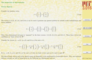
Flatten which would normally turn a list of lists into a (flat) single list. Join is used to collect the
two coordinate lists together into fccsites . The atoms will be visualized with the Sphere graphics
primitive and we use srad to set the radius of a close-packed FCC structure. FCC is a list of (a
list of) graphics primitives for each of the fourteen spheres, and then three cylinders with Opacity
and color are used to define the coordinate axes graphics: axes .
fccmodel is created by joining the spheres and the cylinders, and then using Translate on the
resulting graphics primitives to put the center of the FCC cell at the origin.
2: Translate is an example of a function that operates directly on graphics primitives. We use related
functions that also operate on graphics primitives, Rotate and GeometricTransformation, to
illustrate how rotation by 120◦
about [111], and how inversion (multiplication by “minus the identity
matrix”) followed by the same rotation, are invariant symmetry operations for the FCC lattice.

123. 3.016 Home
Full Screen
Close
Quit
c W. Craig Carter
Sept. 21 2007
Lecture 8: Complex Numbers and Euler’s Formula
Reading:
Kreyszig Sections: 8.1, 8.2, 8.3 (pages334–338, 340–343, 345–348)
Complex Numbers and Operations in the Complex Plane
Consider, the number zero: it could be operationally defined as the number, which when multiplied by any other number
always yields itself; and its other properities would follow.
Negative numbers could be defined operationally as something that gives rise to simple patterns. Multiplying by −1 gives
rise to the pattern 1, −1, 1, −1, . . . In the same vein, a number, ı, can be created that doubles the period of the previous
example: multiplying by ı gives the pattern: 1, ı, −1, −ı, 1, ı, −1, −ı, . . . Combining the imaginary number, ı, with the real
numbers, arbitrarily long periods can be defined by multiplication; applications to periodic phenonena is probably where
complex numbers have their greatest utility in science and engineering
With ı ≡
√
−1, the complex numbers can be defined as the space of numbers spanned by the vectors:
1
0
and
0
ı
(8-1)
so that any complex number can be written as

124. 3.016 Home
Full Screen
Close
Quit
c W. Craig Carter
z = x
1
0
+ y
0
ı
(8-2)
or just simply as
z = x + iy (8-3)
where x and y are real numbers. Rez ≡ x and Imz ≡ y.

125. 3.016 Home
Full Screen
Close
Quit
c W. Craig Carter
Lecture 08 Mathematica R Example 1
Operations on complex numbers
notebook (non-evaluated) pdf (evaluated, color) pdf (evaluated, b&w) html (evaluated)
Straightforward examples of addition, subtraction, multiplication, and division of complex numbers are demonstrated. An example
that demonstrates that Mathematica R doesn’t make a priori assumptions about whether a symbol is real or complex. An example
function that converts a complex number to its polar form is constructed.
1imaginary = Sqrt@-1D
2H-imaginaryL^2
Complex numbers are composed of a real part + an imaginary part
3z1 = a + Â b;
z2 = c + Â d;
4compadd = z1 + z2;
5compmult = z1 * z2;
6Simplify@compmult, a œ Reals &&
b œ Reals && c œ Reals && d œ Reals D
Mathematica does not assume that symbols are necessarily real...
7Re@compaddD
Im@compaddD
However, the Mathematica function ComplexExpand does assume that
the variables are real....
8ComplexExpand@Re@compaddDD
9ComplexExpand@Im@compaddDD
10ComplexExpand@Re@z1 ê z2DD
11ComplexExpand@compmultD
12ComplexExpand@Re@z1^3DD
ComplexExpand@Im@z1^3DD
Function to convert to Polar Form
13Pform@z_D := Abs@zD Exp@Â Arg@zDD
Note: the function Arg[z] returns an angle in the range -p to p which
measures the inclination of z with respect to the +Re axis in the complex
plane.
14Pform@z1D
15Pform@z1 ê. 8a Ø 2, b Ø -p<D
16ComplexExpand@Pform@z1DD
1–2: Just like Pi is a mathematical constant, the imaginary number is defined in Mathematica R as
something with the properties of ı
3: Here, two numbers that are potentially, but not necessarily complex are defined.
4–5: Addition and multiplication are defined as for any symbol; here the results do not appear to be very
interesting because the other symbols could themselves be complex. . .
6: And, Simplify doesn’t help much even with assumptions.
7: The real and imaginary parts of a complex entity can be extracted with Re and Im. This demon-
strates that Mathematica R hasn’t made assumptions about a, b, c, and d.
8-12: However, ComplexExpand does make assumptions that symbols are real and, here, demonstrate
the rules for addition, multiplication, division, and exponentiation.
13–16: Abs calculates the magnitude (also known as modulus or absolute value) and Arg calculates the
argument (or angle) of a complex number. Here, they are used to define a function (Pform ) to
convert and expression to an equivalent polar form of a complex number.

126. 3.016 Home
Full Screen
Close
Quit
c W. Craig Carter
Complex Plane and Complex Conjugates
Because the complex basis can be written in terms of the vectors in Equation 8-1, it is natural to plot complex numbers
in two dimensions—typically these two dimensions are the “complex plane” with (0, ı) associated with the y-axis and (1, 0)
associated with the x-axis.
The reflection of a complex number across the real axis is a useful operation. The image of a reflection across the real axis
has some useful qualities and is given a special name—“the complex conjugate.”
(0, i)
(1, 0)
z=x + iy z=x + iy
z=x ! iy!z=!x ! iy
!z= !x + iy
Re z
Im z
Figure 8-3: Plotting the complex number z in the complex plane: The complex conjugate
(¯z) is a reflection across the real axis; the minus (−z) operation is an inversion through the
origin; therefore −(¯z) = ¯(−z) is equivalent to either a reflection across the imaginary axis or an
inversion followed by a reflection across the real axis.
The real part of a complex number is the projection of the displacement in the real direction and
also the average of the complex number and its conjugate: Rez = (z+¯z)/2. The imaginary part
is the displacement projected onto the imaginary axis, or the complex average of the complex
number and its reflection across the imaginary axis: Imz = (z − ¯z)/(2ı).

127. 3.016 Home
Full Screen
Close
Quit
c W. Craig Carter
Polar Form of Complex Numbers
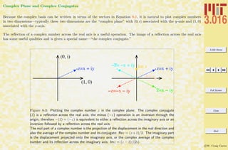
There are physical situations in which a transformation from Cartesian (x, y) coordinates to polar (or cylindrical) coordinates
(r, θ) simplifies the algebra that is used to describe the physical problem.
An equivalent coordinate transformation for complex numbers, z = x + ıy, has an analogous simplifying effect for multiplica-
tive operations on complex numbers. It has been demonstrated how the complex conjugate, ¯z, is related to a reflection—
multiplication is related to a counter-clockwise rotation in the complex plane. Counter-clockwise rotation corresponds to
increasing θ.
The transformations are:
(x, y) → (r, θ)
x = r cos θ
y = r sin θ
(r, θ) → (x, y)
r = x2 + y2
θ = arctan y
x
(8-4)
where arctan ∈ (−π, π].
Multiplication, Division, and Roots in Polar Form
One advantage of the polar complex form is the simplicity of multiplication operations:
DeMoivre’s formula:
zn
= rn
(cos nθ + ı sin nθ) (8-5)
n
√
z = n
√
z(cos
θ + 2kπ
n
+ ı sin
θ + 2kπ
n
) (8-6)

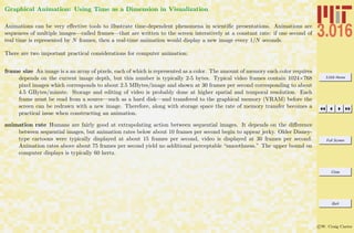
128. 3.016 Home
Full Screen
Close
Quit
c W. Craig Carter
Lecture 08 Mathematica R Example 2
Numerical Properties of Operations on Complex Numbers
notebook (non-evaluated) pdf (evaluated, color) pdf (evaluated, b&w) html (evaluated)
Several examples demonstrate issues that arise when complex numbers are evaluated numerically.
1ExactlyOne = Exp@2 p ÂD
2NumericallyOne = Exp@N@2 p ÂDD
3Chop@NumericallyOneD
4Round@NumericallyOneD
5ExactlyI = Exp@p  ê 2D
6NumericallyI = Exp@N@p  ê 2DD
7Round@NumericallyID
8Chop@NumericallyID
9
ExactlyOnePlusI =
ComplexExpandB 2 Exp@p  ê 4DF
10
NumericallyOnePlusI =
ComplexExpandB 2 Exp@N@p  ê 4DDF
11Chop@NumericallyOnePlusID
12Round@NumericallyOnePlusID
13Round@1.5 - 3.5 Sqrt@-1DD
14Re@NumericallyOnePlusID
15Im@NumericallyOnePlusID
1: The relationship e2πi
= 1 is exact.
2: However, e2.0πi
is numerically 1.
3: Chop removes small evalues that are presumed to be the result of numerical imprecision; it operates
on complex numbers as well.
4: Round is useful for mapping a number to a simpler one in its neighborhood (such as the nearest
integer).
5–8: Here, the difference between something that is exactly ı and is numerically 1.0×ı is demonstrated. . .
[: 9–15] And, this is similar demostration for 1 + ı using its polar form as a starting point.

129. 3.016 Home
Full Screen
Close
Quit
c W. Craig Carter
Exponentiation and Relations to Trignometric Functions
Exponentiation of a complex number is defined by:
ez
= ex+iy
= ex
(cos y + ı sin y) (8-7)
Exponentiation of a purely imaginary number advances the angle by rotation:
eıy
= cos y + ı sin y (8-8)
combining Eq. 8-8 with Eq. 8-7 gives the particularly useful form:
z = x + ıy = reıθ
(8-9)
and the useful relations (obtained simply by considering the complex plane’s geometry)
e2πı = 1 eπı = −1 e−πı = −1 e
π
2
ı
= ı e− π
2
ı
= −ı (8-10)
Subtraction of powers in Eq. 8-8 and generalization gives known relations for trigonometric functions:
cos z =
eız + e−ız
2
sin z =
eız − e−iz
2ı
cosh z =
ez + e−z
2
sinh z =
ez − e−z
2
cos z = cosh ız ı sin z = sinh ız
cos ız = cosh z sin ız = ı sinh z
(8-11)
Complex Numbers in Roots to Polynomial Equations
Complex numbers frequently arise when solving for the roots of a polynomial equation. There are many cases in which
a model of system’s physical behavior depends on whether the roots of a polynomial are real or imaginary, and if the
real part is positive. While evaluating the nature of the roots is straightforward conceptually, this often creates difficulties
computationally. Frequently, ordered lists of solutions are maintained and the behavior each solution is followed.

130. 3.016 Home
Full Screen
Close
Quit
c W. Craig Carter
Lecture 08 Mathematica R Example 3
Complex Roots of Polynomial Equations
notebook (non-evaluated) pdf (evaluated, color) pdf (evaluated, b&w) html (evaluated)
Here we construct an artificial example of a model that depends on a single parameter in a quadratic polynomial and illustrate methods
to analyze and visualize its roots. Methods to “peek” at the form of long expressions are also demonstrated.
1sols = Solve@Hx^4 - x^3 + x + 1L ã 0, xD
2x ê. sols
3Im@x ê. solsD
4ComplexExpand@Im@x ê. solsDD
5ComplexExpand@Im@x ê. solsDD êê N
6ComplexExpand@Re@x ê. solsDD êê N
Generalize the above to a family of solutions.
7bsols = Solve@Hx^4 - x^3 + b * x + 1L ã 0, xD
8Dimensions@bsolsD
Short@bsols, 4D
9SolsbImag = ComplexExpand@Im@x ê. bsolsDD;
10Dimensions@SolsbImagD
Short@SolsbImag@@1DDD
11SolsbReal = ComplexExpand@Re@x ê. bsolsDD;
12Plot@Evaluate@SolsbImagD, 8b, -10, 10<D
13Plot@Evaluate@SolsbImagD, 8b, -10, 10<,
PlotStyle Ø Table@8Hue@1 - a ê 6D<, 8a, 1, 4<DD
14Plot@Evaluate@SolsbRealD, 8b, -10, 10<,
PlotStyle Ø Table@8Hue@1 - a ê 6D<, 8a, 1, 4<DD
15
Plot@Evaluate@SolsbRealD, 8b, -10, 10<,
PlotStyle Ø Table@8Hue@1 - a ê 6D,
Thickness@0.05 - .01 * aD<, 8a, 1, 4<DD
16Plot@Evaluate@x ê. bsolsD,
8b, -10, 10<, PlotStyle Ø ThickD
1–6: Using a prototype fourth order equation, a list of solutions are obtained; the real and imaginary
parts are computed.
7: The above is generalized to a single parameter b in the quartic equation; the conditions that the
roots are real will be visualized. bsols, the list of solution rule-lists is long and complicated.
8: First, one must consider the structure of bsols. Dimensions indicates it is a list of four lists, each
of length 1. Dimensions and Short used together, provides a practical method to observe the
structure of a complicated expression without filling up the screen display.
9–11: Here, the real and complex parts of each of the solutions is obtained with Re and Im where the
parameter b is assumed to be real via the use of ComplexExpand. These may take a long time
to evaluate on some computers.
12–13: Which of the solutions (i.e., 1,2,3, or 4) is identified by a different color (if Evaluate is used
inside the Plot function). In the first case, Mathematica R ’s default indexed colors are used, and
in the second case they are set explicitely using Hue in PlotStyle.
14: Similarly, the real parts appear to converge to a single value when the imaginary parts (from above)
appear. . .
15: But, the actual behavior is best illustrated by using Thickness to distinguish superimposed values.
The behavior of real parts of this solution have what is called a pitchfork structure.
16: As of Mathematica R 6, it is not necessary that the plotted function evaluate to a real value at
each point. Now, only those points that evaluate to a real number will be graphed.

131. 3.016 Home
Full Screen
Close
Quit
c W. Craig Carter
Oct. 3 2007
Lecture 9: Eigensystems of Matrix Equations
Reading:
Kreyszig Sections: 8.1, 8.2, 8.3 (pages334–338, 340–343, 345–348)
Eigenvalues and Eigenvectors of a Matrix
The conditions for which general linear equation
Ax = b (9-1)
has solutions for a given matrix A, fixed vector b, and unknown vector x have been determined.
The operation of a matrix on a vector—whether as a physical process, or as a geometric transformation, or just a general
linear equation—has also been discussed.
Eigenvalues and eigenvectors are among the most important mathematical concepts with a very large number of applications
in physics and engineering.
An eigenvalue problem (associated with a matrix A) relates the operation of a matrix multiplication on a particular vector x
to its multiplication by a particular scalar λ.
Ax = λx (9-2)
This equation bespeaks that the matrix operation can be replaced—or is equivalent to—a stretching or contraction of the
vector: “A has some vector x for which its multiplication is simply a scalar multiplication operation by λ.” x is an eigenvector
of A and λ is x’s associated eigenvalue.

132. 3.016 Home
Full Screen
Close
Quit
c W. Craig Carter
The condition that Eq. 9-2 has solutions is that its associated homogeneous equation:
(A − λI)x = 0 (9-3)
has a zero determinant:
det(A − λI) = 0 (9-4)
Eq. 9-4 is a polynomial equation in λ (the power of the polynomial is the same as the size of the square matrix).
The eigenvalue-eigenvector system in Eq. 9-2 is solved by the following process:
1. Solve the characteristic equation (Eq. 9-4) for each of its roots λi.
2. Each root λi is used as an eigenvalue in Eq. 9-2 which is solved for its associated eigenvector xi

133. 3.016 Home
Full Screen
Close
Quit
c W. Craig Carter
Lecture 09 Mathematica R Example 1
Calculating Matrix Eigenvalues and Eigenvectors
notebook (non-evaluated) pdf (evaluated, color) pdf (evaluated, b&w) html (evaluated)
The symbolic computation of eigenvalues and eigenvectors is demonstrated for simple 2 × 2 matrices. This example is illustrative—more
interesting uses would be for larger matrices. In this example, a “cheat” is employed so that a matrix with “interesting” eigenvalues and
eigenvectors is used as computation fodder.
1mymatrix = 882 + Pi, -2 + Pi<, 8-2 + Pi, 2 + Pi<<;
mymatrix êê MatrixForm
K
2 + p -2 + p
-2 + p 2 + p
O
Solve the characteristic equation for the two eigenvalues:
2Solve@
Det@mymatrix - l IdentityMatrix@2DD ã 0, lD
Compute the eigenvectors:
3Eigenvectors@mymatrixD
48evec1, evec2< = Eigenvectors@mymatrixD
Eigensystem will solve for eigenvalues and corresponding eigenvectors
in one step:
5Eigensystem@mymatrixD
882 p, 4<, 881, 1<, 8-1, 1<<<
Note the output format above: the first item in the list is a list of the two
eigenvalues; the second item in the list is a list of the two corresponding
eigenvectors. Thus, the eigenvector corresponding 2 p is (1,1).
1: A “typical” 2 × 2 matrix mymatrix is defined for the calculations that follow. We will calculate its
eigenvalues directly and with a built-in function.
2: Its eigenvalues can be obtained by by using Solve for the characteristic equation Eq. 9-4 in terms
of λ.
3: And, its eigenvectors could be obtained by putting each eigenvalue back into Eq. 9-2 and then solving
x for each unique λ. However, this tedious procedure can also be performed with Eigenvectors
4: Here, a matrix of eigenvectors is defined with named rows evec1 and evec2.
5: Eigensystem generates the same results as Eigenvectors and Eigenvalues in one step.

134. 3.016 Home
Full Screen
Close
Quit
c W. Craig Carter
The matrix operation on a vector that returns a vector that is in the same direction is an eigensystem. A physical system
that is associated can be interpreted in many different ways:
geometrically The vectors x in Eq. 9-2 are the ones that are unchanged by the linear transformation on the vector.
iteratively The vector x that is processed (either forward in time or iteratively) by A increases (or decreases if λ < 1) along
its direction.
In fact, the eigensystem can be (and will be many times) generalized to other interpretations and generalized beyond linear
matrix systems.
Here are some examples where eigenvalues arise. These examples generalize beyond matrix eigenvalues.
• As an analogy that will become real later, consider the “harmonic oscillator” equation for a mass, m, vibrating with a
spring-force, k, this is simply Newton’s equation:
m
d2x
dt2
= kx (9-5)
If we treat the second derivative as some linear operator, Lspring on the position x, then this looks like an eigenvalue
equation:
Lspringx =
k
m
x (9-6)
• Letting the positions xi form a vector x of a bunch of atoms of mass mi, the harmonic oscillator can be generalized to
a bunch of atoms that are interacting as if they were attached to each other by springs:
mi
d2xi
dt2
=
i’s near neighbors j
kij(xi − xj) (9-7)

135. 3.016 Home
Full Screen
Close
Quit
c W. Craig Carter
For each position i, the j-terms can be added to each side, leaving and operator that looks like:
Llattice =














m1
d2
dt2 −k12 0 −k14 . . . 0
−k21 m2
d2
dt2 −k23 0 . . . 0
...
...
...
... mi
d2
dt2
...
...
mN−1
d2
dt2 −kN−1 N
0 0 . . . −kN N−1 mN
d2
dt2














(9-8)
The operator Llattice has diagonal entries that have the spring (second-derivative) operator and one off-diagonal entry
for each other atom that interacts with the atom associated with row i. The system of atoms can be written as:
k−1
Llatticex = x (9-9)
which is another eigenvalue equation and solutions are constrained to have unit eigenvalues—these are the ‘normal
modes.’
• To make the above example more concrete, consider a system of three masses connected by springs.

136. 3.016 Home
Full Screen
Close
Quit
c W. Craig Carter
Figure 9-4: Four masses connected by three springs
The equations of motion become:





m1
d2
dt2 −k12 −k13 −k14
−k12 m2
d2
dt2 0 0
−k13 0 m2
d2
dt2 0
−k14 0 0 m2
d2
dt2









x1
x2
x3
x4



 =




k12 + k13 + k14 0 0 0
0 k12 0 0
0 0 k13 0
0 0 0 k14








x1
x2
x3
x4



 (9-10)
which can be written as
L4×4x = kx (9-11)

137. 3.016 Home
Full Screen
Close
Quit
c W. Craig Carter
or
k−1
L4×4x = x (9-12)
As will be discussed later, this system of equations can be “diagonalized” so that it becomes four independent equations.
Diagonalization depends on finding the eigensystem for the operator.
• The one-dimensional Shr¨odinger wave equation is:
−
2m
d2ψ(x)
dx2
+ U(x)ψ(x) = Eψ(x) (9-13)
where the second derivative represents the kinetic energy and U(x) is the spatial-dependent potential energy. The
“Hamiltonian Operator” H = −2m
d2
dx2 +U(x), operates on the wave-function ψ(x) and returns the wave-function’s total
energy multiplied by the wave-vector;
Hψ(x) = Eψ(x) (9-14)
This is another important eigenvalue equation (and concept!)
Symmetric, Skew-Symmetric, Orthogonal Matrices
Three types of matrices occur repeatedly in physical models and applications. They can be placed into three categories
according to the conditions that are associated with their eigenvalues:
All real eigenvalues Symmetric matrices—those that have a ”mirror-plane” along the northwest–southeast diagonal (A =
AT
)—must have all real eigenvalues.
Hermitian matrices—the complex analogs of symmetric matrices—in which the reflection across the diagonal is combined
with a complex conjugate operation (aij = ¯aji), must also have all real eigenvalues.
All imaginary eigenvalues Skew-symmetric (diagonal mirror symmetry combined with a minus) matrices (−A = AT
)
must have all complex eigenvalues.
Skew-Hermitian matrices—-the complex analogs of skew-symmetric matrices (aij = − ¯aji)—have all imaginary eigen-
values.

138. 3.016 Home
Full Screen
Close
Quit
c W. Craig Carter
Unitary Matrices: unit determinant Real matrices that satisfy AT
= A−1
have the property that product of all the
eigenvalues is ±1. These are called orthogonal matrices and they have orthonormal rows. Their determinants are also
±1.
This is generalized by complex matrices that satisfy ¯A
T
= A−1
. These are called unitary matrices and their (complex)
determinants have magnitude 1. Orthogonal matrices, A, have the important physical property that they preserve the
inner product: x · y = (Ax) · (Ay). When the orthogonal matrix is a rotation, the interpretation is that the vectors
maintain their relationship to each other if they are both rotated.

139. 3.016 Home
Full Screen
Close
Quit
c W. Craig Carter
Imaginary axis: (0, i)
Real Axis (1, 0)
|!|=1
Unitary
Hermitian
Skew!Hermitian
Figure 9-5: The Symmetric (complex Hermetic), Skew-Symmetric (complex Skew-Hermitian),
Orthogonal, and Unitary Matrix sets characterized by the position of their eigenvalues in the
complex plane. (Hermits live alone on the real axis; Skew-Hermits live alone on the imaginary
axis)
Orthogonal Transformations
Multiplication of a vector by an orthogonal matrix is equivalent to an orthogonal geometric transformation on that vector.
For orthogonal transformation, the inner product between any two vectors is invariant. That is, the inner product of two
vectors is always the same as the inner product of their images under an orthogonal transformation. Geometrically, the

140. 3.016 Home
Full Screen
Close
Quit
c W. Craig Carter
projection (or the angular relationship) is unchanged. This is characteristic of a rotation, or a reflection, or an inversion.
Rotations, reflections, and inversions are orthogonal transformations. The product of orthogonal matrices is also an orthogonal
matrix.

141. 3.016 Home
Full Screen
Close
Quit
c W. Craig Carter
Lecture 09 Mathematica R Example 2
Coordinate Transformations to The Eigenbasis
notebook (non-evaluated) pdf (evaluated, color) pdf (evaluated, b&w) html (evaluated)
Here we demonstrate that a matrix, composed of columns of constructed eigenvectors of a matrix, can be used to diagonalize a matrix,
and the resulting diagonal entries are the matrix eigenvalues.
1simtrans = 8evec2, evec1< êê Transpose;
simtrans êê MatrixForm
2Inverse@simtransD.mymatrix.simtrans êê
Simplify êê MatrixForm
Ù Shows that the transformation to the diagonal basis is a rotation of p/4
Ù Which makes sense considering in initialization steps that mymatrix was
created with a rotation on p/4 of a diagonal matrix
The next command produces an orthonormal basis of the eigenspace
(i.e., the eigenvectors are of unit magnitude):
3Orthogonalize@Eigenvectors@mymatrixD,
Method Ø "GramSchmidt"D êê MatrixForm
The command RotationTransform computes a matrix that will rotate
vectors ccw about the origin in two dimensions, by a specified angle:
4
RotationTransformB
p
4
F@881, 0<, 80, 1<<D êê
MatrixForm
This last result shows that the transformation to the eigenvector space
involves rotation by p/4--and that the matrix corresponding to the eigenvec-
tors produces this same transformation
Here is a demonstration of the general result A xi = li xi , where x is an
eigenvector and l its corresponding eigenvalue:
5evec1
evec2
6mymatrix.evec1
7mymatrix.evec2
MatrixPower multiplies a matrix by itself n times…
8MatrixPower@mymatrix, 12D.evec2 êê Simplify
1: The matrix simtrans is constructed by assigning rows defined by the eigenvectors from the previous
example and then transposing ( Transpose) so that the eigenvectors are the columns.
2: The original matrix is left-multiplied by the inverse of simtrans and right-multiplied by simtrans ;
the result will be a diagonal matrix with the original matrix’s eigenvalues as diagonal entries.
3: The eigenvectors are already orthogonal. There is a process called Gram-Schmidt orthogonalization
used to define a set of vectors that are normal to each other. These orthogonalized vectors form
a convenient basis Linear combinations of the basis vectors can produce any other vector in same
vector space; for the orthogonalized basis, the basis vectors are as independent as possible. Here,
GramSchmidt produces vectors that are also normalized to unit vectors. This, and other useful vector
functions such as Normalize are available for common vector operations.
4: The geometrical interpretation of this operation can be found by comparing a matching
MatrixTransform to the matric composed of eigenvector columns. Here, we see that eigenvector-
matrix is equivalent to the π/4 rotation matrix.
6–7: These demonstrate that Eq. 9-2 is true.
8: This demonstrates that An
x = λn
x.

142. 3.016 Home
Full Screen
Close
Quit
c W. Craig Carter
Oct. 5 2007
Lecture 10: Real Eigenvalue Systems; Transformations to Eigenbasis
Reading:
Kreyszig Sections: 8.4, 8.5 (pages349–354, 356–361)
Similarity Transformations
A matrix has been discussed as a linear operation on vectors. The matrix itself is defined in terms of the coordinate system
of the vectors that it operates on—and that of the vectors it returns.
In many applications, the coordinate system (or laboratory) frame of the vector that gets operated on is the same as the
vector gets returned. This is the case for almost all physical properties. For example:
• In an electronical conductor, local current density, J, is linearly related to the local electric field E:
ρJ = E (10-1)
• In a thermal conductor, local heat current density is linearly related to the gradient in temperature:
k T = jQ (10-2)
• In diamagnetic and paramagnetic materials, the local magnetization, B is related to the applied field, H:
µH = B (10-3)

143. 3.016 Home
Full Screen
Close
Quit
c W. Craig Carter
• In dielectric materials, the local total polarization, D, is related to the applied electric field:
κE = D = κoE + P (10-4)
When x and y are vectors representing a physical quantity in Cartesian space (such as force F, electric field E, orientation of
a plane ˆn, current j, etc.) they represent something physical. They don’t change if we decide to use a different space in which
to represent them (such as, exchanging x for y, y for z, z for x; or, if we decide to represent length in nanometers instead of
inches, or if we simply decide to rotate the system that describes the vectors. The representation of the vectors themselves
may change, but they stand for the same thing.
One interpretation of the operation Ax has been described as geometric transformation on the vector x. For the case of
orthogonal matrices Aorth, geometrical transformations take the forms of rotation, reflection, and/or inversion.
Suppose we have some physical relation between two physical vectors in some coordinate system, for instance, the general
form of Ohm’s law is:
J =σE


Jx
Jy
Jz

 =


σxx σxy σxz
σxy σyy σyz
σxz σyz σzz




Ex
Ey
Ez


(10-5)
The matrix (actually it is better to call it a rank-2 tensor) σ is a physical quantity relating the amount of current that flows
(in a direction) proportional to the applied electric field (perhaps in a different direction). σ is the “conductivity tensor” for
a particular material.
The physical law in Eq. 10-5 can be expressed as an inverse relationship:
E =ρj


Ex
Ey
Ez

 =


ρxx ρxy ρxz
ρxy ρyy ρyz
ρxz ρyz ρzz




jx
jy
jz


(10-6)
where the resistivity tensor ρ = σ−1.

144. 3.016 Home
Full Screen
Close
Quit
c W. Craig Carter
What happens if we decide to use a new coordinate system (i.e., one that is rotated, reflected, or inverted) to describe the
relationship expressed by Ohm’s law?
The two vectors must transform from the “old” to the “new” coordinates by:
Aold→new
orth Eold = Enew Aold→new
orth jold = jnew
Anew→old
orth Enew = Eold Anew→old
orth jnew = jold
(10-7)
Where is simple proof will show that:
Aold→new
orth =Anew→old
orth
−1
Anew→old
orth =Aold→new
orth
−1
Anew→old
orth =Aold→new
orth
T
Anew→old
orth =Aold→new
orth
T
(10-8)
where the last two relations follow from the special properties of orthogonal matrices.
How does the physical law expressed by Eq. 10-5 change in a new coordinate system?
in old coordinate system: jold = χold
Eold
in new coordinate system: jnew = χnew
Enew
(10-9)
To find the relationship between χold and χnew: For the first equation in 10-9, using the transformations in Eqs. 10-7:
Anew→old
orth jnew = χold
Anew→old
orth Enew (10-10)
and for the second equation in 10-9:
Aold→new
orth jold = χnew
Aold→new
orth Eold (10-11)

145. 3.016 Home
Full Screen
Close
Quit
c W. Craig Carter
Left-multiplying by the inverse orthogonal transformations:
Aold→new
orth Anew→old
orth jnew = Aold→new
orth χold
Anew→old
orth Enew
Anew→old
orth Aold→new
orth jold = Anew→old
orth χnew
Aold→new
orth Eold
(10-12)
Because the transformation matrices are inverses, the following relationship between similar matrices in the old and new
coordinate systems is:
χold
= Aold→new
orth χnew
Anew→old
orth
χnew
= Anew→old
orth χold
Aold→new
orth
(10-13)
The χold is said to be similar to χnew and the double multiplication operation in Eq. 10-13 is called a similarity transformation.
Stresses and Strains
Stresses and strains are rank-2 tensors that characterize the mechanical state of a material.
A spring is an example of a one-dimensional material—it resists or exerts force in one direction only. A volume of material
can exert forces in all three directions simultaneously—and the forces need not be the same in all directions. A volume of
material can also be “squeezed” in many different ways: it can be squeezed along any one of the axis or it can be subjected
to squeezing (or smeared) around any of the axes4
All the ways that a force can be applied to small element of material are now described. A force divided by an area is a
stress—think of it the area density of force.
σij =
Fi
Aj
(i.e., σxz =
Fx
Az
= σxz =
F ·ˆi
A · ˆk
) (10-14)
Aj is a plane with its normal in the ˆj-direction (or the projection of the area of a plane A in the direction parallel to ˆj)
4
Consider a blob of modeling clay—you can deform it by placing between your thumbs and one opposed finger; you can deform it by simultaneously
squeezing with two sets of opposable digits; you can “smear” it by pushing and pulling in opposite directions. These are examples of uniaxial, biaxial,
and shear stress.

146. 3.016 Home
Full Screen
Close
Quit
c W. Craig Carter
x
y
z
!yx
!zx
!xx
!yy
!zy
!xy
!yz
!zz
!xz
!21
!31
!11
!22
!32
!12
!23
!33
!13
Figure 10-6: Illustration of stress on an oriented volume element.
σij =


σxx σxy σxz
σyx σyy σyz
σzx σzy σzz

 (10-15)
There is one special and very simple case of elastic stress, and that is called the hydrostatic stress. It is the case of pure
pressure and there are no shear (off-diagonal) stresses (i.e., all σij = 0 for i = j, and σ11 = σ22 = σ33). An equilibrium system
composed of a body in a fluid environment is always in hydrostatic stress:
σij =


−P 0 0
0 −P 0
0 0 −P

 (10-16)
where the pure hydrostatic pressure is given by P.
Strain is also a rank-2 tensor and it is a physical measure of a how much a material changes its shape.5
5
It is unfortunate that the words of these two related physical quantities, stress and strain, sound so similar. Strain measures the change in

147. 3.016 Home
Full Screen
Close
Quit
c W. Craig Carter
Why should strain be a rank-2 tensor?
z
y
x
z
y
x
Lx
Ly
Lz
Figure 10-7: Illustration of how strain is defined: imagine a small line-segment that is aligned
with a particular direction (one set of indices for the direction of the line-segment); after defor-
mation the end-points of the line segment define a new line-segment in the deformed state. The
difference in these two vectors is a vector representing how the line segment has changed from
the initial state into the deformed state. The difference vector can be oriented in any direction
(the second set of indices)—the strain is a representation of “a difference vectors for all the
oriented line-segments” divided by the length of the original line.
Or, using the same idea as that for stress:
ij =
∆Li
Lj
(i.e., xz =
∆Lx
Lz
= xz =
∆L ·ˆi
L · ˆk
) (10-17)
geometry of a body and stress measures the forces that squeeze or pull on a body. Stress is the press; Strain is the gain.

148. 3.016 Home
Full Screen
Close
Quit
c W. Craig Carter
If a body that is being stressed hydro-statically is isotropic, then its response is pure dilation (in other words, it expands or
shrinks uniformly and without shear):
ij =


∆/3 0 0
0 ∆/3 0
0 0 ∆/3

 (10-18)
∆ =
dV
V
(10-19)
So, for the case of hydrostatic stress, the work term has a particularly simple form:
V
3
i=1
3
j=1
σijd ij = −PdV
V σijd ij = −PdV (summation convention)
(10-20)
This expression is the same as the rate of work performed on a compressible fluid, such as an ideal gas.
EigenStrains and EigenStresses
For any strain matrix, there is a choice of an coordinate system where line-segments that lie along the coordinate axes always
deform parallel to themselves (i.e., they only stretch or shrink, they do not twist).
For any stress matrix, there is a choice of an coordinate system where all shear stresses (the off-diagonal terms) vanish and
the matrix is diagonal.
These coordinate systems define the eigenstrain and eigenstress. The matrix transformation that takes a coordinate system
into its eigenstate is of great interest because it simplifies the mathematical representation of the physical system.

149. 3.016 Home
Full Screen
Close
Quit
c W. Craig Carter
Lecture 10 Mathematica R Example 1
Representations of Stress (or Strain) in Rotated Coordinate Systems
notebook (non-evaluated) pdf (evaluated, color) pdf (evaluated, b&w) html (evaluated)
A demonstration of rotating a quasi-two dimensional stress state is given. Convenient forms for the stress in any coordinate system are
derived. The stress invariants are demonstrated.
This is a general state, we will rotate about the z-axis and compare the
result to a general two-dimensional stress state.
1
stensordiag =
sprincxx 0 0
0 sprincyy 0
0 0 sprinczz
;
stensordiag êê MatrixForm
2
rotmat@q_D :=
Cos@qD -Sin@qD 0
Sin@qD Cos@qD 0
0 0 1
;
rotmat@qD êê MatrixForm
Transformation to general two-dimensional stress state coordinate
system by rotating the principal system by q around z-axis
3
srot = Simplify@Transpose@rotmat@qDD.
stensordiag.rotmat@qDD;
srot êê MatrixForm
Writing the same equation in a slightly different way...
4
srotalt = Collect@
srot êê TrigReduce, 8Cos@2 qD, Sin@2 qD<D;
srotalt êê MatrixForm
Naming the coefficients of the rotated two-dimensional state:
5
slabMat =
slabxx slabxy slabxz
slabxy slabyy slabyz
slabxz slabyz slabzz
= srotalt;
slabMat êê MatrixForm
Looking at the x-y components of stress (i.e, the upper-left 2!2 subma-
trix), notice that there are two invariants of the generalized two-dimen-
sional stress state: The trace and the determinant:
6Simplify@slabxx + slabyy D
7SimplifyAslabxx slabyy - IslabxyM^2E
Do not depend on q; thus illustrating the invariance of these quantities
under rotation of coordinate rotations.
1: The problem is done in reverse by finding the backwards rotation of a diagonal matrix. This is the
stress in the principle coordinate system (it is diagonalized with eigenvalue entries) Any rotation
similarity transformation on this matrix is the equivalent stress in the rotated frame.
2: This is the rotation operator by counter-clockwise angle θ about the z-axis.
3: Therefore σrot, obtained by the similarity transformation, is the stress in any rotation about the
z-axis. It is a quasi-two dimensional state defined by σzx = σyz = 0.
4: The rotation matrix factors well using the double angle formulas; here we use TrigReduce to convert
powers of trigonometric functions into functions of multiples of their angle, and the Collect the
double-angle terms.
5: This can be compared with the general form of any quasi-two-dimensional (x–y plane) stress that
has the same principle stresses identified above. In the rotated (i.e., laboratory) frame, the stresses
are geometrically related to the circle plotted in 10-8, which will be also visualized in the following
examples.
6: Here, we use double assignment for the laboratory-frame matrix and, simultaneously, its elements.
7: This will show that the trace of the stress tensor is independent of rotation—this is a general property
for any unitary transformation.
8: Like the trace, the determinant is also an matrix invariant.

150. 3.016 Home
Full Screen
Close
Quit
c W. Craig Carter
Lecture 10 Mathematica R Example 2
Principal Axes: Mohr’s Circle of Two-Dimensional Stress
notebook (non-evaluated) pdf (evaluated, color) pdf (evaluated, b&w) html (evaluated)
By diagonalizing a quasi-two-dimensional stress tensor, the equations for Mohr’s circle of stress (Fig. 10-8) are derived.
1. slabxx in laboratory system rotated by q from principal axis system
1slabxx
2. slabyy in laboratory system rotated by q from principal axis system
2slabyy
3. slabxy in laboratory system rotated by q from principal axis system
3slabxy
4uniaxial10 = 9sprincxx -> 10, sprincyy -> 0=
5
ParametricPlot@8slabxx, slabxy< ê. uniaxial10
, 8q, 0, p<, AxesLabel Ø
8"normal stress", "shear stress"<,
AspectRatio Ø 1, PlotLabel Ø " t t Mohr
Circle for 10 MPa Uniaxial Tension",
PlotStyle Ø 8Thickness@0.01D, Hue@1D<D
6uniaxialother = 9sprincxx -> 30, sprincyy -> 10=
7
ParametricPlotA
8slabxx, slabxy< ê. uniaxialother
, 8q, 0, p<, AxesLabel Ø 8"normal stress",
"shear stress"<, AspectRatio Ø 1,
PlotRange -> 880, 40<, 8-20, 20<<,
PlotLabel Ø " t t Mohr Circle
for sprincxx= 30 sprincyy=10",
PlotStyle Ø 8Thickness@0.01D, Hue@1D<E
1–3: These are the forms of the three two-dimensional stress components are simple expressions in terms
of 2θ. We will see how these equations produce a circle.
4: This is a rule that defines a particular stress state in terms of the principal stresses (here given by
10 and 0).
5: 5–7 Using ParametricPlot for σxx(θ) and σxy(θ), an example of Mohr’s circle is plotted for examples
of principle stress for (0,10) and (30,10). The interpretation of this figure is given in Fig. 10-8.

151. 3.016 Home
Full Screen
Close
Quit
c W. Craig Carter
!lab
xy
!princ
large
2"
!princ
small
!ii( ")
!j j( ")
!i j( ")
!princ
1 +!princ
2
2
!ii( ") = offset+radiuscos2"
!i j( ") = radiussin2"
where
!j j( ") = offset !radiuscos2"
offset =
!princ
large+!princ
small
2
radius =
!princ
large !!princ
small
2
Figure 10-8: Mohr’s circle of stress is a way of graphically representing the two-dimensional
stresses of identical stress states, but in rotated laboratory frames.
The center of the circle is displaced from the origin by a distance equal to the average of the
principal stresses (or average of the eigenvalues of the stress tensor).
The maximum and minimum stresses are the eigenvalues—and they define the diameter in the
principal θ = 0 frame.
Any other point on the circle gives the stress tensor in a frame rotated by 2θ from the principal
axis using the construction illustrated by the blue lines (and equations).

152. 3.016 Home
Full Screen
Close
Quit
c W. Craig Carter
Lecture 10 Mathematica R Example 3
Visualization Example: Graphics for Mohr’s Circle
notebook (non-evaluated) pdf (evaluated, color) pdf (evaluated, b&w) html (evaluated)
Our goal is to produce a manipulatable and interactive graphical representation for Mohr’s circle of stress. We break the problem up
by creating the individual graphical elements that appear in Fig. 10-8. These functions will be utilized in the following example.
1
mohrs@off_, rad_D :=
8Red, Thick, Circle@8offset, 0<, radiusD<
2
s12graph@s11_, s12_D := 8Darker@OrangeD,
Arrow@88s11, s12<, 80, s12<<D,
Text@s12, 80, s12<,
8-1.5, -1.5<, Background Ø WhiteD<
3
s22graph@s22_, s12_D :=
8Blue, Arrow@88s22, -s12<, 8s22, 0<<D,
Text@s22, 8s22, 0<, 80, -1<,
Background Ø WhiteD<
4
s11graph@s11_, s12_D := 8Darker@GreenD,
Dynamic@Arrow@88s11, s12<, 8s11, 0<<DD,
Dynamic@Text@s11, 8s11, 0<,
80, 1<, Background Ø WhiteDD<
5
diamgraph@s11_, s12_, s22_D :=
8Line@88s22, -s12<, 8s11, s12<<D<
6
anglegraph@twotheta_D :=
8Purple, Dashed, Circle@8offset, 0<,
1.2 * radius, 80, twotheta<D, Text@
Style@"2q=" <> ToString@twotheta 180 ê PiD,
MediumD, 8offset, 0< + 1.2 * radius *
8Cos@twotheta ê 2D, Sin@twotheta ê 2D<,
Background Ø WhiteD<
7
titlegraph@s11_, s12_, s22_D :=
Text@MatrixForm@
88Text@Style@s11, Darker@GreenD, LargeDD,
Text@Style@s12, Darker@OrangeD, LargeDD<,
8Text@Style@s12, Darker@OrangeD, LargeDD,
Text@Style@s22, Blue, LargeDD<<DD
1: The function mohrs will produce graphical primitives at an arbitrary offset=(σxx + σyy)/2 and
radius==(σxx − σyy)/2.
2: This will be an annotated dark orange horizontal arrow for the shear stress value σxy
3: This will be an annotated blue vertical arrow for the stress σyy
4: This will be an annotated dark green vertical arrow for the stress σxx
5: This will illustrate the diameter of the circle in the current θ-orientation.
6: This will annotate the current angle 2θ.
7: This creates a title for the graph with entries colored corresponding to the arrows on the graph.

153. 3.016 Home
Full Screen
Close
Quit
c W. Craig Carter
Lecture 10 Mathematica R Example 4
Interactive Graphics Demonstration for Mohr’s Circle
notebook (non-evaluated) pdf (evaluated, color) pdf (evaluated, b&w) html (evaluated)
We create graphics in which we can use the mouse to drag elements that dynamically update the visualization. In this case, we create
a handle that will allow visualization of two-dimensional stress in an arbitrary rotation. The dynamic graphics are enclosed within
Manipulate so that the original stress state can be set by the user.
1
Manipulate@
offset = Hs11 + s22L ê 2; radius = Hs11 - s22L ê 2;
ThetaInit = ArcSin@s12 ê radiusD ê 2;
DynamicModule@8twotheta = 2 ThetaInit,
s11 = 3, s12 = 4, s22<, LocatorPane@
Dynamic@H8radius Cos@twothetaD + offset,
radius Sin@twothetaD<L,
Htwotheta = Mod@Apply@ArcTan,
HÒ - 8offset, 0<LD, 2 PiDL &D,
s11 = Dynamic@offset + radius
Cos@twothetaDD;
s12 = Dynamic@ radius Sin@twothetaDD;
s22 =
Dynamic@offset - radius Cos@twothetaDD;
Graphics@8mohrs@offset, radiusD,
Dynamic@anglegraph@twothetaDD,
Dynamic@diamgraph@s11, s12, s22DD,
Dynamic@s12graph@s11, s12DD ,
Dynamic@s22graph@s22, s12DD ,
Dynamic@s11graph@s11, s12DD <,
Axes Ø True, AxesOrigin Ø 80, 0<,
PlotLabel Ø
Dynamic@titlegraph@s11, s12, s22DDD
D
D, 88s11 , 8<, -1, 11<,
88s22 , 3.0<, -5, 7<, 88s12 , 2<, -5, 5<,
FrameLabel Ø Text@
Style@"Mohr's Circle of Stress", LargeDDD
1: Manipulate will get sliders for each of σ11, σ22, and σ33 (see note below about these values).
The circle offset, radius, and the value of 2θ are calculated first from the Mohr’s equation formula.
Because we will be changing θ, its current value and the stress state for that rotation will change.
We make these variables local (as in Module), but further specify that they will be dynamically
updated by using DynamicModule.
We use LocatorPane to place a “handle” at a specific spot which can be updated with the mouse.
As the value of θ is changed, we must inform the symbols (here twotheta, s11, s12, and s22) are to
be updated by embedding them in the Dynamic function.
The graphics are drawn using the functions from the previous example.
In this example, no precautions are made to ensure that the stress components will be real in every
orientation.

154. 3.016 Home
Full Screen
Close
Quit
c W. Craig Carter
Quadratic Forms
The example above, where a matrix (rank-2 tensor) represents a material property, can be understood with a useful geometrical
interpretation.
For the case of the conductivity tensor σ, the dot product E · j is a scalar related to the local energy dissipation:
e = ET
σE (10-21)
The term on the right-hand-side is called a quadratic form, as it can be written as:
e =σ11x2
1 + σ12x1x2 + σ13x1x3+
σ21x1x2 + σ22x2
2 + σ23x2x3+
σ31x1x3 + σ32x2x3 + σ33x2
3
(10-22)
or, because σ is symmetric:
e =σ11x2
1 + 2σ12x1x2 + 2σ13x1x3+
σ22x2
2 + 2σ23x2x3+
σ33x2
3
(10-23)
It is not unusual for such quadratic forms to represent energy quantities. For the case of paramagnetic and diamagnetic
materials with magnetic permeability tensor µ, the energy per unit volume due to an applied magnetic field H is:
E
V
=
1
2
HT
µH (10-24)
for a dielectric (i.e., polarizable) material with electric electric permittivity tensor κ with an applied electric field E:
E
V
=
1
2
ET
κE (10-25)

155. 3.016 Home
Full Screen
Close
Quit
c W. Craig Carter
The geometric interpretation of the quadratic forms is obtained by turning the above equations around and asking—what are
the general vectors x for which the quadratic form (usually an energy or power density) has a particular value? Picking that
particular value as unity, the question becomes what are the directions and magnitudes of x for which
1 = xT
Ax (10-26)
This equation expresses a quadratic relationship between one component of x and the others. This is a surface—known as
the quadric surface or representation quadric—which is an ellipsoid or hyperboloid sheet on which the quadratic form takes
on the particular value 1.
In the principal axes (or, equivalently, the eigenbasis) the quadratic form takes the quadratic form takes the simple form:
e = xeb
T
Aebxeb = A11x2
1 + A22x2
2 + A33x2
3 (10-27)
and the representation quadric
A11x2
1 + A22x2
2 + A33x2
3 = 1 (10-28)
which is easily characterized by the signs of the coefficients.
In other words, in the principal axis system (or the eigenbasis) the quadratic form has a particularly simple, in fact the most
simple, form.
Eigenvector Basis
Among all similar matrices (defined by the similarity transformation defined by Eq. 10-13), the simplest matrix is the diagonal
one. In the coordinate system where the similar matrix is diagonal, its diagonal entries are the eigenvalues. The question
remains, “what is the coordinate transformation that takes the matrix into its diagonal form?”
The coordinate system is called the eigenbasis or principal axis system, and the transformation that takes it there is particularly
simple.
The matrix that transforms from a general (old) coordinate system to a diagonalized matrix (in the new coordinate system)
is the matrix of columns of the eigenvectors. The first column corresponds to the first eigenvalue on the diagonal matrix, and
the nth column is the eigenvector corresponding the nth eigenvalue.

156. 3.016 Home
Full Screen
Close
Quit
c W. Craig Carter


The
Diagonalized
Matrix

 =


Eigenvector
Column
Matrix


−1 

The
General
Matrix




Eigenvector
Column
Matrix

 (10-29)
This method provides a method for finding the simplest quadratic form.

157. 3.016 Home
Full Screen
Close
Quit
c W. Craig Carter
Oct. 11 2007
Lecture 11: Geometry and Calculus of Vectors
Reading:
Kreyszig Sections: 9.1, 9.2, 9.3, 9.4 (pages364–369, 371–374, 377–383, 384–388)
Vector Products
The concept of vectors as abstract objects representing a collection of data has already been presented. Every student at this
point has already encountered vectors as representation of points, forces, and accelerations in two and three dimensions.

158. 3.016 Home
Full Screen
Close
Quit
c W. Craig Carter
Review: The Inner (dot) product of two vectors and relation to projection
An inner- (or dot-) product is the multiplication of two vectors that produces a scalar.
a · b ≡
≡aibi
≡aibjδij where δij ≡
1 if i = j
0 otherwise
≡(a1, a2, . . . aN )





b1
b2
...
bN





≡(b1, b2, . . . bN )





a1
a2
...
aN





(11-1)
The inner product is:
linear, distributive (k1a + k2b) · c = k1a · c + k2b · c
symmetric a · b = b · a
satisfies Schwarz inequality a · b ≤ b a
ratifies triangle inequality a + b ≤ b + a
If the vector components are in a Cartesian (i.e., cubic lattice) space, then there is a useful equation for the angle between
two vectors:
cos α =
a · b
a b
= ˆna · ˆnb (11-2)

159. 3.016 Home
Full Screen
Close
Quit
c W. Craig Carter
where ˆni is the unit vector that shares a direction with i. Caution: when working with vectors in non-cubic crystal lattices
(e.g, tetragonal, hexagonal, etc.) the angle relationship above does not hold. One must convert to a cubic system first to
calculate the angles.
The projection of a vector onto a direction ˆnb is a scalar:
p = a · ˆnb (11-3)
Review: Vector (or cross-) products
The vector product (or cross ×) differs from the dot (or inner) product in that multiplication produces a vector from two
vectors. One might have quite a few choices about how to define such a product, but the following idea proves to be useful
(and standard).
normal Which way should the product vector point? Because two vectors (usually) define a plane, the product vector might
as well point away from it.
The exception is when the two vectors are linearly-dependent; in this case the product vector will have zero magnitude.
The product vector is normal to the plane defined by the two vectors that make up the product. A plane has two normals,
but which normal should be picked? By convention, the “right-hand-rule” defines which of the two normals should be
picked.
magnitude Given that the product vector points away from the two vectors that make up the product, what should be its
magnitude? We already have a rule that gives us the cosine of the angle between two vectors, so a rule that gives the
sine of the angle between the two vectors would be useful. Therefore, the cross product is defined so that its magnitude
for two unit vectors is the sine of the angle between them.
This has the extra utility that the cross product is zero when two vectors are linearly-dependent (i.e., they do not define
a plane).
This also has the utility, discussed below, that the triple product will be a scalar quantity equal to the volume of the
parallelepiped defined by three vectors.

160. 3.016 Home
Full Screen
Close
Quit
c W. Craig Carter
The triple product,
a · (b × c) = (a × b) · c =
a b c sin γb−c cos γa−bc =
a b c sin γa−b cos γab−c
(11-4)
where γi−j is the angle between two vectors i and j, and γij−k is the angle between the vector k and the plane spanned by i
and j, is equal to the parallelepiped that has a, b, and c emanating from its bottom-back corner.
If the triple product is zero, the volume between three vectors is zero and therefore they must be linearly dependent.

161. 3.016 Home
Full Screen
Close
Quit
c W. Craig Carter
Lecture 11 Mathematica R Example 1
Cross Product Example
notebook (non-evaluated) pdf (evaluated, color) pdf (evaluated, b&w) html (evaluated)
This is a simple demonstration of the vector product of two spatial vectors.
Here is the built-in cross product between two vectors
1crossab = Cross@8a1, a2, a3< , 8b1, b2, b3<D
And, here is the standard visual way to do it by hand with the determinant.
2detab = DetB
i j k
a1 a2 a3
b1 b2 b3
F
Pick out each of the compenents to create the vector
3
testcrossab = 8Coefficient@detab, iD,
Coefficient@detab, jD,
Coefficient@detab, kD<
Check for equality between the old-fashioned way and Mathematica's
built-in function
4testcrossab ã crossab
1: Cross produces the vector product of two symbolic vectors a and b of length 3.
2: Det produces the same result using the memorization device:
a × b = det
0
@
ˆi ˆj ˆk
a1 a2 a3
b1 b2 b3
1
A
3–4: Coefficient is used to extract each vector component and create a vector result, and then equality
test the two vectors to show the equivalence.

162. 3.016 Home
Full Screen
Close
Quit
c W. Craig Carter
Lecture 11 Mathematica R Example 2
Visualizing Space-Curves as Time-Dependent Vectors
notebook (non-evaluated) pdf (evaluated, color) pdf (evaluated, b&w) html (evaluated)
Examples of x(t) and dx/dt are illustrated as curves and as animations.
Create a trajectory of a point or a particle
1
XVector@t_D :=
8Cos@6 tD, Sin@4 t D, Sin@tD + Cos@tD<
ParametricPlot3D allows us to visualize the entire trajectory at once.
2
ParametricPlot3D@XVector@tD,
8t, 0, 2 p<, PlotStyle Ø 8Thick, Blue<,
AxesLabel Ø 8"x", "y", "z"<D
Here is a function to create a graphic with a variable end - point. We will
have the function remember when it has already computed a graphic,
trading memory for a possible speed-up.
3
paraplot@time_D := paraplot@timeD =
ParametricPlot3D@XVector@tD,
8t, 0, time<, PlotStyle Ø 8Thick, Blue<,
AxesLabel Ø 8"x", "y", "z"<D
Use manipulate on the graphics function to visualize how the curve
develops with its parameter
4Manipulate@paraplot@timeD,
88time, 0.05<, 0.01, 2 p<D
However, we need to fix the length scale between frames, so we use the
last graphic to infer what PlotRange should be.
5
Manipulate@Show@paraplot@timeD,
PlotRange Ø 88-1, 1<, 8-1, 1<, 8-1.5, 1.5<<D,
88time, 0.05<, 0.01, 2 p<D
Next, we add a graphic element to show the vector, drawn from the
origin, for each end-point.
6
Manipulate@
Show@8paraplot@timeD, Graphics3D@8Cylinder@
880, 0, 0<, XVector@timeD<, 0.03D<D<,
PlotRange Ø 88-1, 1<, 8-1, 1<, 8-1.5, 1.5<<D,
88time, 0.05<, 0.01, 2 p<D
1: A list of three time-dependent components for (x, y, z) is constructed as the function XVector .
2: ParametricPlot3D takes a three-component vector as an argument and then will plot the evolution
of the vector as a function of a parameter.
3: To visualize the evolution of the curve, it is useful to plot the resulting trajectory. We create a
function that constructs a plot up to a variable end-point, time, which appears as the upper-bound
to ParametricPlot3D.
4: Manipulate provides an interactive animation of the curve’s development.
5: However, it is better if the length scale is fixed. We set PlotRange from visual inspection of the last
frame of the previous example.
6: To improve the visualization, we add a Cylinder graphics primitive to illustrate the vector drawn
from the origin.

163. 3.016 Home
Full Screen
Close
Quit
c W. Craig Carter
Derivatives of Vectors
Consider a vector, p, as a point in space. If that vector is a function of a real continuous parameter, for instance, t, then p(t)
represents the loci as a function of a parameter.
If p(t) is continuous, then it sweeps out a continuous curve as t changes continuously. It is very natural to think of t as
time and p(t) as the trajectory of a particle—such a trajectory would be continuous if the particle does not disappear at one
instant, t, and then reappear an instant later, t + dt, some finite distance distance away from p(t).
If p(t) is continuous, then the limit is:
dp(t)
dt
= lim
∆t→0
p(t + ∆t) − p(t)
∆t
(11-5)
Notice that the numerator inside the limit is a vector and the denominator is a scalar; so, the derivative is also a vector. Think
about the equation geometrically—it should be apparent that the vector represented by the derivative is locally tangent to
the curve that is traced out by the points p(t − dt), p(t) p(t + dt), etc.

164. 3.016 Home
Full Screen
Close
Quit
c W. Craig Carter
Lecture 11 Mathematica R Example 3
Visualizing Time-Dependent Vectors and their Derivatives
notebook (non-evaluated) pdf (evaluated, color) pdf (evaluated, b&w) html (evaluated)
Examples of x(t) and dx/dt are illustrated as curves and as animations.
The local derivative of the vector that we visualized above: v =
d x
dt
1Simplify@D@XVector@tD, tDD
Write out a function for the derivative:
2
dxdt@s_D :=
8-6 Sin@6 sD, 4 Cos@4 sD, Cos@sD - Sin@sD<
3
dxdtplot@time_D :=
ParametricPlot3D@dxdt@tD, 8t, 0, time<,
PlotStyle Ø 8Thick, Darker@RedD<,
AxesLabel Ø 8"x", "y", "z"<D
dxdtplot@2 pD
4
Manipulate@
Show@paraplot@timeD, dxdtplot@timeD,
Graphics3D@8
8Lighter@BlueD, Cylinder@
880, 0, 0<, XVector@timeD<, 0.1D<,
8Lighter@RedD, Cylinder@
880, 0, 0<, dxdt@timeD<, 0.1D<
<D, PlotRange Ø 88-6, 6<, 8-4, 4<,
8-1.5, 1.5<<D, 88time, 0.05<, 0.01, 2 p<D
To visualize the "tangency property," we translate the derivative-vector to
the end of the space curve
5
Manipulate@
Show@paraplot@timeD, dxdtplot@timeD,
Graphics3D@8
8Lighter@BlueD, Cylinder@
880, 0, 0<, XVector@timeD<, 0.1D<,
8Lighter@RedD, Translate@
Cylinder@880, 0, 0<, dxdt@timeD<, 0.1D,
XVector@timeDD<
<D, PlotRange Ø 88-6, 6<, 8-6, 6<,
8-4, 4<<D, 88time, 0.05<, 0.01, 2 p<D
1: The derivative operator D is a threadable function so it will operate on each component of its vector
argument; thus, we can obtain the vector derivative by operating on the entire vector.
2: The derivative-vector dx/dt is encoded as a function.
3: The derivative of the space-curve (from the above example) is visualized with a function that calls
ParameticPlot3D. Because the space curve is differentiable and periodic, its derivative should be
periodic as well, but it appears to not be periodic.
4: Using Manipulate reveals that the function is periodic.
5: Here, we repeat the interactive example, but use Translate to move the visualized derivative-vector
to the end of the curve. This will give a visual demonstration of the tangent behavior of the derivative.

165. 3.016 Home
Full Screen
Close
Quit
c W. Craig Carter
Review: Partial and total derivatives
One might also consider that a time- and space-dependent vector field, for instance E(x, y, z, t) = E(x, t) could be the force
on a unit charge located at x and at time t.
Here, there are many different things which might be varied and which give rise to a derivative. Such questions might be:
1. How does the force on a unit charge differ for two nearby unit-charge particles, say at (x, y, z) and at (x, y + ∆y, z)?
2. How does the force on a unit charge located at (x, y, z) vary with time?
3. How does the force on a particle change as the particle traverses some path (x(t), y(t), z(t)) in space?
Each question has the “flavor” of a derivative, but each is asking a different question. So a different kind of derivative should
exist for each type of question.
The first two questions are of the nature, “How does a quantity change if only one of its variables changes and the others are
held fixed?” The kind of derivative that applies is the partial derivative.
The last question is of the nature “How does a quantity change when all of its variables depend on a single variable?” The
kind of derivative that applies is the total derivative. The answers are:
1.
∂E(x, y, z, t)
∂y
=
∂E
∂y
constantx,z,t
(11-6)
2.
∂E(x, y, z, t)
∂t
=
∂E
∂t
constantx,y,z
(11-7)

166. 3.016 Home
Full Screen
Close
Quit
c W. Craig Carter
3.
dE(x(t), y(t), z(t), t)
dt
=
∂E
∂x
dx
dt
+
∂E
∂y
dy
dt
+
∂E
∂z
dz
dt
+
∂E
∂t
dt
dt
= E(x(t), t) ·
dx
dt
+
∂E
∂t
(11-8)
Time-Dependent Scalar and Vector Fields
A physical quantity that is spatially variable is often called a spatial field. It is a particular case of a field quantity.
Such fields can be simple scalars, such as the altitude as a function of east and west in a topographical map. Vectors can
also be field quantities, such as the direction uphill and steepness on a topographical map— this is an example of how each
scalar field is naturally associated with its gradient field. Higher dimensional objects, such as stress and strain, can also be
field quantities.
Fields that evolve in time are time-dependent fields and appear frequently in physical models. Because time-dependent 3D
spatial fields are four-dimensional objects, animation is frequently used to visualize them.
For a working example, consider the time-evolution of “ink concentration” c(x, y, t) of a very small spot of ink spilled on
absorbent paper at x = y = 0 and at time t = 0. This example could be modeled with Fick’s first law:
J = −D c(x, y, t) = −D
∂c
∂x
+
∂c
∂y
(11-9)
where D is the diffusivity that determines “how fast” the ink moves for a given gradient c, and J is a time-dependent vector
that represents “rate of ink flow past a unit-length line segment oriented perpendicular to J. This leads to the two-dimensional
diffusion equation
∂c
∂t
= D
∂2c
∂x2
+
∂2c
∂y2
(11-10)
For this example, the solution, c(x, y, t) is given by
c(x, y, t) =
co
4πDt
e− x2+y2
4Dt (11-11)
where co is the initial concentration of ink.

167. 3.016 Home
Full Screen
Close
Quit
c W. Craig Carter
Lecture 11 Mathematica R Example 4
Visualizing a Solution to the Diffusion Equation
notebook (non-evaluated) pdf (evaluated, color) pdf (evaluated, b&w) html (evaluated)
The solution to a 2D diffusion equation in the infinite plane with rectangular initial conditions c(−a/2 < x < a/2, −b/2 < y < b/2, t =
0) = 1 and c(|x| > a/2, |y| > b/2, t = 0) = 0 is visualized and will serve as an example of the flux (or time-dependent gradient) field in
the following example.
1
concentration =
IntegrateB
ExpB
-HHxsource-xL^2 + Hysource-yL^2L
4 Diffusivity t
F
4 Pi Diffusivity t
,
8xsource, -a ê 2, a ê 2<,
8ysource, -b ê 2, b ê 2<,
Assumptions Ø Diffusivity > 0 && t > 0 &&
a > 0 && b > 0 && x œ Reals && y œ RealsF
2
aspectRatio = 3;
b = aspectRatio a;
length = a;
time = length^2 ê Diffusivity;
ScaleRules =
8t -> t time, x -> x length, y -> h length<;
3
scaledconc =
Simplify@concentration ê. ScaleRules,
Assumptions Ø a > 0D
4
Plot3D@scaledconc ê. t Ø 0.003,
8x, -3, 3<, 8h, -3, 3<, PlotRange Ø 80, 1<,
MeshFunctions Ø 8Ò3 &<, PlotPoints Ø 30,
Mesh Ø 5, MeshStyle Ø 8Thick<D
5
Manipulate@Plot3D@scaledconc ê. t Ø timevar,
8x, -3, 3<, 8h, -3, 3<,
PlotRange Ø 80, 1<, MaxRecursion Ø 4D,
88timevar, 0.05<, 0.001, 0.1<D
6
cplots =
Table@ContourPlot@scaledconc ê. t Ø timevar,
8x, -3, 3<, 8h, -3, 3<,
PlotRange Ø 80, 1<, ColorFunction Ø
ColorData@"TemperatureMap"DD,
8timevar, .001, .2, .005<D;
7ListAnimate@cplotsD
1: This is the solution to the stated problem. It is obtained by integrating the appropriate Green’s
function which will be discussed in a later lecture. We use physical Assumptions in the call to
Integrate.
2: We set a model parameter (aspectRatio) for the shape of the initial rectangle, and then define a
characteristic length and time in terms of quantities that appear in the model. A set of rules
are defined, ScaleRules , that can be applied to the solution to create a non-dimensional model the
problem.
3: The re-scaled solution, scaledconc , depends only on non-dimensional quantities, ξ, η, and τ.
4: Here is an example of the solution at τ = 0.003. We use the MeshFunctions option to Plot3D to
draw the five isoconcentration lines on the surface.
5: This will produce an interactive animation of the solution. However, because the evaluation of each
animation-frame is likely to be slow, this visualization will be sluggish on many computers.
6: A simpler graphical representation is obtained with ContourPlot by plotting contours of constant
concentration. We pre-compute a table of plots and store the result.
7: The resulting animation is created from two-dimensional objects using ListAnimate on the pre-
computed frames.

168. 3.016 Home
Full Screen
Close
Quit
c W. Craig Carter
Lecture 11 Mathematica R Example 5
Visualizing the Diffusion Flux: The Time-Dependent Gradient Field
notebook (non-evaluated) pdf (evaluated, color) pdf (evaluated, b&w) html (evaluated)
The time-dependent gradient field for the 2D diffusion equation treated above is visualized.
1flux = 8-D@scaledconc, xD, -D@scaledconc, hD<
2Needs@"VectorFieldPlots`"D;
3
VectorFieldPlot@flux ê. t Ø .08,
8x, -3, 3<, 8h, -3, 3<, PlotPoints Ø 21,
ColorFunction Ø ColorData@"DarkRainbow"DD
4
vplots =
Table@VectorFieldPlot@flux ê. t Ø time,
8x, -3, 3<, 8h, -3, 3<, PlotPoints Ø 21,
PlotRange Ø 88-4, 4<, 8-4, 4<<,
Frame Ø True, MaxArrowLength Ø 3,
ScaleFactor Ø None,
ScaleFunction Ø H2 Ò &L,
ColorFunction Ø HHue@0.25 + 0.75 ÒD &LD,
8time, .001, .2, .005<D;
5ListAnimate@vplotsD
6
ListAnimate@
Table@Show@cplots@@iDD, vplots@@iDD,
PlotRange Ø 3.5 88-1, 1<, 8-1, 1<<,
ImageSize Ø 872, 72<D,
8i, 1, Length@cplotsD<DD
1: The flux, J, is the rate of matter-flow through an oriented plane per unit area. Fick’s first law
related the flux to the gradient of the concentration field, J = −D c. Here, we compute a non-
dimensionalized form of flux.
2: To plot the flux which is a vector field, the package VectorFieldPlots is loaded so that we have
access to its PlotVectorField function. For example, here is an example of (minus) the gradient
field at τ = 0.08. The vectors are plotted on a square mesh and we color them according to their
magnitude with ColorFunction and ColorData.
5–6: We precompute a series of frames and animate them. To ensure that the vector length scales are
consistent between frames, the option ScaleFactor is used.
7: Here, we visualize time-dependent vector flux and the concentration together by using Show on
pre-computed graphics.

169. 3.016 Home
Full Screen
Close
Quit
c W. Craig Carter
All vectors are not spatial
It is useful to think of vectors as spatial objects when learning about them—but one shouldn’t get stuck with the idea that
all vectors are points in two- or three-dimensional space. The spatial vectors serve as a good analogy to generalize an idea.
For example, consider the following chemical reaction:
Reaction: H2
1
2 O2 H2O
Initial: 1 1 0
During Rx.: 1 − ξ 1 − 1
2 ξ ξ
The composition could be written as a vector:
N =


moles H2
moles O2
moles H2O

 =


1 − ξ
1 − 1
2 ξ
ξ

 (11-12)
and the variable ξ plays the role of the “extent” of the reaction—so the composition variable N lives in a reaction-extent (ξ)
space of chemical species.

170. 3.016 Home
Full Screen
Close
Quit
c W. Craig Carter
Oct. 12 2007
Lecture 12: Multivariable Calculus
Reading:
Kreyszig Sections: 9.5, 9.6, 9.7 (pages389–398, 400–403, 403–409)
The Calculus of Curves
In the last lecture, the derivatives of a vector that varied continuously with a parameter, r(t), were considered. It is natural
to think of r(t) as a curve in whatever space the vector r is defined. The most familiar example is a curve in the plane:
the two values (x(t), y(t)) are mapped onto the plane through values as t sweeps through its range tinitial ≤ t ≤ tfinal. A
curve in three-dimensional Cartesian space is the mapping of three values (x(t), y(t), z(t)); and in cylindrical coordinates it
is: (r(t), θ(t), z(t)). In general, a curve is represented by N coordinates, as a single parameter (i.e., t) takes on a range of
numbers—the N coordinates form the embedding space.
Objects that have more dimensions than curves need more parameters. The number of parameters is the dimensionality of the
object and the number of coordinates is the dimensionality of the embedding space. What we naturally call a surface is a two
dimensional object embedded in a three-dimensional space—for example, in Cartesian coordinates (x(u, v), y(u, v), z(u, v)) is
a surface.
The two-dimensional surface (x(u, v), y(u, v), z(u, v)) can itself become an embedding space for lower dimensional objects; for
example, the curve (u(t), v(t)) is embedded in the surface (u, v) which itself is embedded in (x, y, z). In other words, the curve
(x(u(t), v(t)), y(u(t), v(t)), z(u(t), v(t))) can be considered to be embedded in (u, v), or embedded in (x, y, z) and constrained
to the surface (x(u, v), y(u, v), z(u, v)).
In higher dimensions, there are many more possibilities and we can make a few introductory remarks about the language that
is used to describe them. For application to physical problems, these considerations indicate the number of degrees-of-freedom

171. 3.016 Home
Full Screen
Close
Quit
c W. Craig Carter
that are available and the conditions that a system is over-constrained. An N-dimensional surface (sometimes called a hyper-
surface) embedded in an M-dimensional space is said to have codimension M − N. Some objects cannot be embedded in a
higher dimensional space; these are called non-embeddable, and examples include the Klein bottle which cannot be embedded
in our three-dimensional space.

172. 3.016 Home
Full Screen
Close
Quit
c W. Craig Carter
Lecture 12 Mathematica R Example 1
Embedding Curves in Surfaces in Three Dimensions
notebook (non-evaluated) pdf (evaluated, color) pdf (evaluated, b&w) html (evaluated)
An example is constructed that visualizes a two-dimensional surface in three dimensions and then visualizes a one-dimensional curve
constrained to that surface.
Create an example function that returns a position {x, y, z} as a function
of two parameters
1
FlowerPot@u_, v_D := 8H3 + Cos@vDL Cos@uD,
Sin@uD + H3 + Cos@vDL Sin@uD,
H3 ê 2 + Cos@u + vDL Sin@vD<
Visualize it.
2
Flowerplot = ParametricPlot3D@
FlowerPot@u, vD, 8u, 0, 2 Pi<,
8v, 0, 2 Pi<, PlotPoints -> 8120, 40<,
PlotStyle Ø Directive@Brown, Opacity@0.6D,
Specularity@White, 40DD, Mesh Ø NoneD
A Curve on a parameritized surface
Now, we call the function again, but make the two parameters {u,v},
depend on a single parameter t (*note when visualizing this curve, it has
been scaled in and out a little so it will be visible in subsequent visualiza-
tions*)
3
Vines@t_D := FlowerPot@t Cos@tD, -t^2 Sin@ tDD
vineplot = ParametricPlot3D@
81.05 * Vines@tD, 0.95 * Vines@tD<,
8t, 0, 2 Pi<, PlotStyle Ø
88Thickness@0.025D, Darker@GreenD<,
8Thickness@0.025D, Darker@GreenD<<,
PlotRange Ø AllD
This is the paramertized surface with a curve embedded in the surface.
4Show@vineplot, FlowerplotD
1: FlowerPot takes two arguments and returns a vector. As the arguments sweep through domains,
the vector will trace out a surface.
2: Using the ParametricPlot3D, the surface is visualized. Here we use Directive to make the surface
brown with Opacity to make the surface about 40% transparent. Specularity is used to make the
surface text look a bit shiny here. The resulting graphics are assigned to the symbol Flowerplot.
3: Vines takes a single argument and then calls FlowerPot with two arguments that are functions of
that single argument—the result must be a curve embedded in the surface. In this case, the function
is repeated and is scaled in and out a little, so the curves will be visible later.
4: Here, both the embedded curve and the surface are shown together.

173. 3.016 Home
Full Screen
Close
Quit
c W. Craig Carter
Because the derivative of a curve with respect to its parameter is a tangent vector, the unit tangent can be defined immediately:
ˆu =
dr
dt
dr
dt
(12-1)
It is convenient to find a new parameter, s(t), that would make the denominator in Eq. 12-1 equal to one. This parameter,
s(t), is the arc-length:
s(t) =
t
to
ds
=
t
to
dx2 + dy2 + dz2
=
t
to
(
dx
dt
)2 + (
dy
dt
)2 + (
dz
dt
)2dt
=
t
to
(
dr
dt
) · (
dr
dt
)dt
(12-2)
and with s instead of t,
ˆu(s) =
dr
ds
(12-3)
This is natural because r and s have the same units (i.e., meters and meters, foots and feet, etc) instead of, for instance,
time, t, that makes dr/dt a velocity and involves two different kinds of units (e.g., furlongs and hours).
With the arc-length s, the magnitude of the curvature is particularly simple,
κ(s) =
dˆu
ds
=
d2r
ds2
(12-4)
as is its interpretation—the curvature is a measure of how rapidly the unit tangent is changing direction.
Furthermore, the rate at which the unit tangent changes direction is a vector that must be normal to the tangent (because
d(ˆu · ˆu = 1) = 0) and therefore the unit normal is defined by:
ˆp(s) =
1
κ(s)
dˆu
ds
(12-5)

174. 3.016 Home
Full Screen
Close
Quit
c W. Craig Carter
There are two unit vectors that are locally normal to the unit tangent vector ˆu (s) and the curve unit normal ˆp(s) × ˆu
and ˆu(s) × ˆp. This last choice is called the unit binormal, ˆb ≡ ˆu(s) × ˆp and the three vectors together form a nice little
moving orthogonal axis pinned to the curve. Furthermore, there are convenient relations between the vectors and differential
geometric quantities called the Frenet equations.
Using Arc-Length as a Curve’s Parameter
However, it should be pointed out that—although re-parameterizing a curve in terms of its arc-length makes for simple
analysis of a curve—achieving this re-parameterization is not necessarily simple.
Consider the steps required to represent a curve r(t) in terms of its arc-length:
integration The integral in Eq. 12-2 may or may not have a closed form for s(t).
If it does, then we can perform the following operation:
inversion s(t) is typically a complicated function that is not easy to invert, i.e., solve for t in terms of s to get a t(s) that
can be substituted into r(t(s)) = r(s).
These difficulties usually result in treating the problem symbolically and resorting to numerical methods of achieving the
integration and inversion steps.

175. 3.016 Home
Full Screen
Close
Quit
c W. Craig Carter
Lecture 12 Mathematica R Example 2
Calculating arclength
notebook (non-evaluated) pdf (evaluated, color) pdf (evaluated, b&w) html (evaluated)
Examples of computing a curve’s arc-length s from the relation ds = |dx| = (dx2
+ dy2
+ dz2
) are presented.
Make up two functions that will illustrate the difference between a curve's
parameter and its arclength
1
PrettyFlower@t_D :=
1
4
+
3
4
Cos@3 tD
8 Cos@tD^3, Sin@tD^3, Sin@tD Cos@tD^2<
2Bendy@t_ D := 8 Cos@tD, Sin@tD, Sin@tD Cos@tD<
Here is a general way to take a function of a general parameter, t, and
compute the arc length traversed as t varies from one value to another:
3dFlowerDt = Simplify@D@PrettyFlower@tD, tDD
This is the arclength up to the parameter t, the integral does not have a
closed-form
4sFlower = Integrate@
Sqrt@Simplify@dFlowerDt.dFlowerDtDD, tD
In other words,
ds2
= dx2
+ dy2
+ dz2
so integrating
the square root of this is the arclength
Applying this to the function Bendy defined above:
5dBendyDt = D@Bendy@tD, tD
This is the arclength up to the parameter t, the integral does have a
closed-form, but is not easily invertible.
The arc length in this case is given by a tabulated function called an
elliptic integral and after checking its behavior at t = 0 we can plot it over
the range {t,0,2p}:
6sBendy ê. t Ø 0
However, the inverse exits, we can find a t(s) (the curve parameter t for
any arclength s)
7Plot@sBendy, 8t, 0, 2 Pi<D
Alternatively, we can evaluate the expression for arc length numerically
using the following:
8
Plot@Evaluate@
NIntegrate@Sqrt@dFlowerDt.dFlowerDtD,
8t, 0, uplim<DD, 8uplim, 0, 6.4<D
1–2: Two example functions of a single parameter t that return a vector x are defined for this example.
3: Here, the tangent-vector for the function, PrettyFlower defined above, is computed.
4: This is an attempt to find a closed-form solution for arclength s(τ) − s(0) =
R τ
0
q`dc
dt
´2
dt. A
closed-form solution doesn’t exist.
5: However, a closed-form solution does exist for the arclength of the Bendy function defined earlier.
If the closed-form s(t) could be inverted (i.e., t(s)) then the curve c(t) could be expressed in terms
of its natural variable c(s) = c(t(s)).
6–7: The plot, s(t), is monotonically increasing, and therefore the function could always be inverted
numerically.
8: Even for the arc-length that could not be evaluated in closed-form (i.e., PrettyFlower ), a numerical
integration could be used to perform the inversion.

176. 3.016 Home
Full Screen
Close
Quit
c W. Craig Carter
Scalar Functions with Vector Argument
In Materials Science and Engineering, the concept of a spatially varying function arises frequently:
For example:
Concentration ci(x, y, z) = ci(x) is the number (or moles) of chemical species of type i per unit volume located at the point
x.
Density ρ(x, y, z) = ρ(x) mass per unit volume located at the point x is ρ(x, y, z) = ρ(x).
Energy Density u(x, y, z) = u(x) energy per unit volume located at the point x.
The examples above are spatially-dependent densities of “extensive quantities.”
There are also spatially variable intensive quantities:
Temperature T(x, y, z) = T(x) is the temperature which would be measured at the point x.
Pressure P(x, y, z) = P(x) is the pressure which would be measured at the point x.
Chemical Potential µi(x, y, z) = µi(x) is the chemical potential of the species i which would be measured at the point x.
Each example is a scalar function of space—that is, the function associates a scalar with each point in space.
A topographical map is a familiar example of a graphical illustration of a scalar function (altitude) as a function of location
(latitude and longitude).

177. 3.016 Home
Full Screen
Close
Quit
c W. Craig Carter
How Confusion Can Develop in Thermodynamics
However, there are many other types of scalar functions of several arguments, such as the state function: U = U(S, V, Ni) or
P = P(V, T, Ni). It is sometimes useful to think of these types of functions a scalar functions of a “point” in a thermodynamics
space.
However, this is often a source of confusion: notice that the internal energy is used in two different contexts above. One
context is the value of the energy, say 128.2 Joules. The other context is the function U(S, V, Ni). While the two symbols are
identical, their meanings are quite different.
The root of the confusion lurks in the question, “What are the variables of U?” Suppose that there is only one (independent)
chemical species, then U(·) has three variables, such as U(S, V, N). “But if S(T, P, µ), V (T, P, µ), and N(T, P, µ) are known
functions, then what are the variables of U?” The answer is that they are any three independent variables, one could write
U(T, P, µ) = U(S(T, P, µ), V (T, P, µ), N(T, P, µ)), and there are six other natural choices.
The trouble arises when variations of a function like U are queried—then the variables that are varying must be specified.
For this reason, it is either a good idea to keep the functional form explicit in thermodynamics, i.e.,
dU(S, V, N) =
∂U(S, V, N)
∂S
dS +
∂U(S, V, N)
∂V
dV +
∂U(S, V, N)
∂N
dN
dU(T, P, µ) =
∂U(T, P, µ)
∂T
dT +
∂U(T, P, µ)
∂V
dV +
∂U(T, P, µ)
∂µ
dµ
(12-6)
or use, the common thermodynamic notation,
dU =
∂U
∂S V,N
dS +
∂U
∂V S,N
dV +
∂U
∂N S,V
dN
dU =
∂U
∂T P,µ
dT +
∂U
∂P T,µ
dP +
∂U
∂µ T,P
dµ
(12-7)

178. 3.016 Home
Full Screen
Close
Quit
c W. Craig Carter
Total and Partial Derivatives, Chain Rule
There is no doubt that a great deal confusion arises from the following question, “What are the variables of my function?”
For example, suppose we have a three-dimensional space (x, y, z), in which there is an embedded surface (x(w, v), y(w, v), z(w, v))
x(w, v) = x(u) where u = (v, w) is a vector that lies in the surface, and an embedded curve (x(s), y(s), z(s)) = x(s). Further-
more, suppose there is a curve that lies within the surface (w(t), v(t)) = u(t).
Suppose that E = f(x, y, z) is a scalar function of (x, y, z).
Here are some questions that arise in different applications:
1. How does E vary as a function of position?
2. How does E vary along the surface?
3. How does E vary along the curve?
4. How does E vary along the curve embedded in the surface?

179. 3.016 Home
Full Screen
Close
Quit
c W. Craig Carter
Lecture 12 Mathematica R Example 3
Total Derivatives and Partial Derivatives: A Mathematica Review
notebook (non-evaluated) pdf (evaluated, color) pdf (evaluated, b&w) html (evaluated)
Demonstrations of 1) the three spatial derivatives of F(x, y, z); 2) the two independent derivatives on a two-dimensional surface embedded
in x–y–z; 3) the complete derivative of F(x, y, z) along a curve (x(t), y(t), z(t)).
AScalarFunction is defined everywhere in (x,y,z)
1
AScalarFunction@x_ , y_ , z_D :=
SomeFunction@x, y, zD
2AScalarFunction@x, y, zD
The following lines print and they define expressions.
3
dFuncX = D@AScalarFunction@x, y, zD, xD
dFuncY = D@AScalarFunction@x, y, zD, yD
dFuncZ = D@AScalarFunction@x, y, zD, zD
x(w,v), y(w,v), z(w,v) is a restriction of all space to a surface parameter-
ized by (w,v),
AScalarFunction is now defined on the surface as a function of (w,v)
4AScalarFunction@x@w, vD, y@w, vD, z@w, vDD
Because it is now a function of w and v, the derivative with respect to x
will vanish:
5D@AScalarFunction@
x@w, vD, y@w, vD, z@w, vDD, xD
Two more flavors of derivatives, these are partial derivatives evaluated
on the surface
6dFuncW = D@AScalarFunction@
x@w, vD, y@w, vD, z@w, vDD, wD
7dFuncV = D@AScalarFunction@
x@w, vD, y@w, vD, z@w, vDD, vD
On the surface x(w,v), y(w,v), z(w,v), we can prescribe a curve w(t), v(t),
.now we have AScalarFunction defined on that curve
8AScalarFunction@x@w@tD, v@tDD,
y@w@tD, v@tDD, z@w@tD, v@tDDD
The following is a derivative of the function along the curve parameter-
ized by t
9dFuncT = D@AScalarFunction@x@w@tD, v@tDD,
y@w@tD, v@tDD, z@w@tD, v@tDDD, tD
10dFuncT =
D@AScalarFunction@x@tD, y@tD, z@tDD, tD
1–2: AScalarFunction is a symbolic representation of a function—it will be a place-holder for examples
of partial derivatives.
3: This will print Mathematica’s representation of derivatives with respect to one of several arguments—
e.g., ∂F(x, y, z)/∂y is written as F(0,1,0)
[x,y,z].
4: AScalarFunction becomes a function of two variables when x, y, and z are restricted to a surface
parameterized by (u, v): (x(w, v), y(w, v), z(w, v))
5–6: Caution: the distinction between the symbol x and the symbol x[w,v] is important; the following
two examples show how the derivatives should appear.
7: This and the previous example show how the chain rule is computed, these two terms are the
components of the gradient in the surface.
8: In this case, the previous AScalarFunction becomes a function of a single variable by specifying a
curve in the surface with (w(t), v(t)).
9: Now, a total derivative of the curve embedded in the surface can be calculated with the chain rule.
This is nearly equivalent to the following along a specified curve.
10: Here is the total derivative along a specific curve (x(t), y(t), z(t), but here there is no constraint to
the surface x(w, v)

180. 3.016 Home
Full Screen
Close
Quit
c W. Craig Carter
Taylor Series
The behavior of a function near a point is something that arises frequently in physical models. When the function has
lower-order continuous partial derivatives (generally, a “smooth” function near the point in question), the stock method to
model local behavior is Taylor’s series expansions around a fixed point.
Taylor’s expansion for a scalar function of n variables, f(x1, x2, . . . , xn), which has continuous first and second partial deriva-
tives near the point ξ = (ξ1, ξ2, . . . , ξn), is:
f(ξ1, ξ2, . . . , ξn) = f(x1, x2, . . . , xn)
+
∂f
∂x1 ξ
(ξ1 − x1) +
∂f
∂x2 ξ
(ξ2 − x2) + . . . +
∂f
∂xn ξ
(ξn − xn)
+
1
2
[
∂2f
∂x1
2
ξ
(ξ1 − x1)2
) +
∂2f
∂x1∂x2 ξ
(ξ1 − x1)(ξ2 − x2) + . . . +
∂2f
∂x1∂xn ξ
(ξ1 − x1)(ξn − xn)
+
∂2f
∂x2∂x1 ξ
(ξ2 − x2)(ξ1 − x1) +
∂2f
∂x2
2
ξ
(ξ2 − x2)2
+ . . . +
∂2f
∂x2∂xn ξ
(ξ2 − x2)(ξn − xn)
... . . .
...
+
∂2f
∂xn∂x1 ξ
(ξn − xn)(ξ1 − x1) +
∂2f
∂xn∂x2 ξ
(ξn − xn)(ξ2 − x2) + . . . +
∂2f
∂xn
2
ξ
(ξn − xn)2
]
+ O (ξ1 − x1)3
+ O (ξ1 − x1)2
(ξ2 − x2) + O (ξ1 − x1)(ξ2 − x2)2
+ O (ξ2 − x2)3
+ . . . + O (ξ1 − x1)2
(ξn − xn) + O [(ξ1 − x1)(ξ2 − x2)(ξn − xn)] + . . . + O (ξn − xn)3
(12-8)
or in a vector shorthand:
f(x) = f(ξ) + xf|ξ
· (ξ − x) + (ξ − x) · ( x xf)|ξ
· (xi − x) + O ξ − x 3
(12-9)

181. 3.016 Home
Full Screen
Close
Quit
c W. Craig Carter
In the following example, visualization of local approximations will be obtained for a scalar function of two variables, f(x, y).
This will be extended into an approximating function of four variables by expanding it about a point (ξ, η) to second order.
The expansion is now a function of four variables—the first two variables are the point the function is expanded around
(x and y), and the second two are the variable of the parabolic approximation at that point (ξ and η): fappx(ξ, η; x, y) =
f(x, y)+ ∂f
∂x x,y
(ξ −x)+ ∂f
∂y x,y
(η −y)+Q where Q ≡ 1
2
∂2f
∂x2
x,y
(ξ −x)(ξ −x)+ ∂2f
∂x∂y x,y
(ξ −x)(η −y)+ 1
2
∂2f
∂y2
x,y
(η −y)(η −y)
or fappx(ξ, η, x, y) = f(x, y) + f ·
ξ − x
η − y
+ 1
2 Qform where Qform ≡ (ξ − x, η − y)


∂2f
∂x2
x,y
∂2f
∂x∂y x,y
∂2f
∂y∂x x,y
∂2f
∂y2
x,y

 ξ − x
η − y
The function fappx(ξ, η, x, y) will be plotted as a function of ξ and η for |ξ − x| < δ and |η − y| < δ for a selected number of
points (x, y).

182. 3.016 Home
Full Screen
Close
Quit
c W. Craig Carter
Lecture 12 Mathematica R Example 4
Taylor Expansions of a Scalar Function of v in the Neighborhood of Zero
notebook (non-evaluated) pdf (evaluated, color) pdf (evaluated, b&w) html (evaluated)
This will demonstrate how to produce an expression-form for a first-order expansion to a function of three variables.
This is symbolic representation of a first order expansion (keeping all
terms) of a function near x,y,z
1
SmallChangeSeries =
Expand@Series@AScalarFunction@x + dx,
y + dy, z + dzD, 8dx, 0, 1<, 8dy, 0, 1<,
8dz, 0, 1<DD - AScalarFunction@x, y, zD
Using normal converts the approximation into an expression, but higher
order terms are still present
2dScalarFunction =
Expand@Normal@SmallChangeSeriesDD
The next step eliminates second- and third-order terms… (remember, dx,
dy, and dz are small)
3dScalarFunction = dScalarFunction ê.
8dx dy Ø 0, dy dz Ø 0, dx dz Ø 0<
dz SomeFunctionH0,0,1L
@x, y, zD +
dy SomeFunctionH0,1,0L
@x, y, zD +
dx SomeFunctionH1,0,0L
@x, y, zD
The above form is like the thermodynamic expression :
dF =
! F
! x
dx +
! F
! y
dy +
! F
! z
dz
1: Here, we get a symbolic representation of the approximation of F(x + dx, y + dy, z + dz) near the
point (x, y, z) = (0, 0, 0) to first order. The Series function first expands about the last iterator-
argument. This produces a result that multiplies the expansion parameters dx, dy, and dz by the
order of approximation functions O[dx2
].
2: Using Normal and Expand on the series-result above yields an expression for the approximation, but
it is not first-order as we might have intended. The dx dy-terms are a result of expanding the result
of the three sequential expansions in the first command.
3: Here, a rule is applied to remove the second-order terms. The result has the same form as the
thermodynamic expression:
dG =
„
∂G
∂P
«
T,n
dP +
„
∂G
∂T
«
n,P
+
„
∂G
∂n
«
P,T
= V (P, T, n)dP − S(P, T, n)dT + µ(P, T, n)dn

183. 3.016 Home
Full Screen
Close
Quit
c W. Craig Carter
Lecture 12 Mathematica R Example 5
Approximating Surfaces at Points
notebook (non-evaluated) pdf (evaluated, color) pdf (evaluated, b&w) html (evaluated)
Visualization of quadratic approximations to a surface at points on that surface
1
CrazyFun@x_, y_D :=
Sin@5 p xD Sin@5 p yD ê Hx yL + Sin@5 p Hx - 1LD
Sin@5 p Hy - 1LD ê HHx - 1L H y - 1LL
2
theplot = Plot3D@CrazyFun@x, yD,
8x, 0.1, .9<, 8y, 0.1, .9<, PlotRange Ø All,
Mesh Ø False, PlotStyle Ø 8Opacity@0.5D<D
3
Approxfunction@x_, y_ , xo_ , yo_D :=
Series@CrazyFun@x, yD,
8x, xo, 2<, 8y, yo, 2<D êê Normal
4
anapprox = Plot3D@
Evaluate@Approxfunction@x, y, .7, .1DD,
8x, .7 - .1, .7 + .1<, 8y, .1 - .1, .1 + .1<D
5Show@ theplot, anapproxD
6Table@8xo@iD = RandomReal@D,
yo@iD = RandomReal@D<, 8i, 1, 100<D;
7
ApproxPlot@i_D := Plot3D@Evaluate@
Approxfunction@x, y, xo@iD, yo@iDDD,
8x, xo@iD - .1, xo@iD + .1<,
8y, yo@iD - .1, yo@iD + .1<, PlotPoints Ø 6,
Mesh Ø True, ColorFunction Ø
HRGBColor@0.9 xo@iD, 0.9 yo@iD, ÒD &LD
8GraphicsStack@1D = Show@ApproxPlot@1DD;
9
GraphicsStack@i_D := GraphicsStack@iD =
Show@GraphicsStack@i - 1D, ApproxPlot@iDD
10Manipulate@Show@theplot, GraphicsStack@iDD,
88i, 3<, 1, 20, 1<D
1–2: CrazyFun is an example scalar function of two variables.
3–4: Using Normal to convert the Taylor Expansion obtained by Series at a point xo, yo produces
a function Approxfunction of four variables (the point it is approximated (xo, yo) and the local
expansion variables at that point (x, y)).
5: This illustrates how the local quadratic approximation fits the surface locally at a particular point
(0.7, 0.7) in a square of (half)-side-length 0.1
6: Generate a list of random points at which to visualize the local approximation.
7: ApproxPlot is an example that will plot the local approximation for any indexed random point. The
surface is colored by using the value of the point as an indicator.
8-9: This is an example of producing a stack of graphics with a recursive graphics function. It iteratively
adds a new approximating surface graphics object to the set of the previous ones.
10: This will produce a visualization of approximations at different parts of the original surface.

184. 3.016 Home
Full Screen
Close
Quit
c W. Craig Carter
Just a few of many examples of instances where Taylor’s expansions are used are:
linearization Examining the behavior of a model near a point where the model is understood. Even if the model is wildly
non-linear, a useful approximation is to make it linear by evaluating near a fixed point.
approximation If a model has a complicated representation in terms of unfamiliar functions, a Taylor expansion can be
used to characterize the ‘local’ model in terms of a simple polynomial.
asymptotics Even when a system has singular behavior (e.g, the value of a function becomes infinite as some variable
approaches a particular value), how the system becomes singular is very important. At singular points, the Taylor
expansion will have leading order terms that are singular, for example near x = 0,
sin(x)
x2
=
1
x
−
x
6
+ O(x3
) (12-10)
The singularity can be subtracted off and it can be said that this function approaches ∞ ”linearly” from below with
slope -1/6. Comparing this to the behavior of another function that is singular near zero:
exp(x)
x
=
1
x
+ 1 +
x
2
+
x2
6
+ O(x3
) (12-11)
shows that the ex/x behavior is “more singular.”

185. 3.016 Home
Full Screen
Close
Quit
c W. Craig Carter
Plot
Sin x
x^2
1
x
,
Exp x
x
1
x
, x, .001, 2.5 ,
PlotStyle Thickness 0.02 , Hue 1 , Thickness 0.01 , Hue 0.5
0.5 1 1.5 2 2.5
1
2
3
4
Graphics
Figure 12-9: Behavior of two singular functions near their singular points.
stability If the expansion of energy about a point is obtained, then the various orders of expansion can be interpreted:
zero-order The zeroth-order term in a local expansion is the energy of the system at the point evaluated. Unless this
term is to be compared to another point, it has no particular meaning (if it is not infinite), as energy is always

186. 3.016 Home
Full Screen
Close
Quit
c W. Craig Carter
arbitrarily defined up to a constant.
first-order The first-order is related to the driving force to change the state of the system. Consider:
∆E = E · δx = −F · δx (12-12)
If force exists, the system can decrease its energy linearly by picking a particular change δx that is anti-parallel to
the force.
For a system to be stable, it is a necessary first condition that the forces (or first order expansion
coefficients) vanish.
second order If a system has no forces on it (therefore satisfying the necessary condition of stability), then where the
system is stable or unstable depends on whether a small δx can be found that deceases the energy:
∆E =
1
2
δx · −F · δx
=
1
2
· E · δx
=
1
2
∂2E
∂xi∂xj x1,x2,...xn
δxiδxj
(12-13)
where the summation convention is used above and the point (x1, x2, . . . , xn) is one for which E is zero.
numerics Derivatives are often obtained numerically in numerical simulations. The Taylor expansion provides a formula
to approximate numerical derivatives—and provides an estimate of the numerical error as a function of quantities like
numerical mesh size.
Gradients and Directional Derivatives
Scalar functions F(x, y, z) = F(x) have a natural vector field associated with them—at each point x there is a direction ˆn(x)
pointing in the direction of the most rapid increase of F. Associating the magnitude of a vector in the direction of steepest
increase with the rate of increase of F defines the gradient.
The gradient is therefore a vector function with a vector argument (x in this case) and it is commonly written as F.

187. 3.016 Home
Full Screen
Close
Quit
c W. Craig Carter
Here are some natural examples:
Meteorology The “high pressure regions” are commonly displayed with weather reports—as are the ”isobars” or curves of
constant barometric pressure. Thus displayed, pressure is a scalar function of latitude and longitude.
At any point on the map, there is a direction that points to a local high pressure center—this is the direction of the
gradient. The rate at which the pressure is increasing gives the magnitude of the gradient.
The gradient of pressure should be a vector that is related to the direction and the speed of wind.
Mosquitoes It is known that hungry mosquitoes tend to fly towards sources (or local maxima) of carbon dioxide. Therefore,
it can be hypothesized that mosquitoes are able to determine the gradient in the concentration of carbon dioxide.
Heat In an isolated system, heat flows from high-temperature (T(x)) regions to low-temperature regions.
The Fourier empirical law of heat flow states that the rate of heat flows is proportional to the local decrease in temper-
ature.
Therefore, the local rate of heat flow should be proportional to the vector which is minus the gradient of T(x): − T
Finding the Gradient
Potentials and Force Fields
Force is a vector. Force projected onto a displacement vector dx is the rate at which work, dW, is done on an object
dW = −F · dx.
If the work is being supplied by an external agent (e.g., a charged sphere, a black hole, a magnet, etc.), then it may be possible
to ascribe a potential energy (E(x), a scalar function with vector argument) to the agent associated with the position at which
the force is being applied.6 This E(x) is the potential for the agent and the force field due to the agent is F(x) = − E(x).
6
As with any energy, there is always an arbitrary constant associated with the position (or state) at which the energy is taken to be zero. There
is no such ambiguity with force. Forces are, in a sense, more fundamental than energies. Energy appears to be fundamental because all observations
of the first law of thermodynamics demonstrate that there is a conserved quantity which is a state function and is called energy.

188. 3.016 Home
Full Screen
Close
Quit
c W. Craig Carter
Sometimes the force (and therefore the energy) scales with the “size” of the object (i.e., the object’s total charge in an electric
potential due to a fixed set of charges, the mass of an object in the gravitational potential of a black hole, the magnetization
of the object in a magnetic potential, etc.). In these cases, the potential field can be defined in terms of a unit size (per unit
charge, per unit mass, etc.). One can determine whether such a scaling is applied by checking the units.

189. 3.016 Home
Full Screen
Close
Quit
c W. Craig Carter
Oct. 15 2007
Lecture 13: Differential Operations on Vectors
Reading:
Kreyszig Sections: 9.8, 9.9 (pages410–413, 414–416)
Generalizing the Derivative
The number of different ideas, whether from physical science or other disciplines, that can be understood with reference to
the “meaning” of a derivative from the calculus of scalar functions, is very very large. Our ideas about many topics, such as
price elasticity, strain, stability, and optimization, are connected to our understanding of a derivative.
In vector calculus, there are generalizations to the derivative from basic calculus that act on a scalar and give another scalar
back:
gradient ( ): A derivative on a scalar that gives a vector.
curl ( ×): A derivative on a vector that gives another vector.
divergence ( ·): A derivative on a vector that gives scalar.
Each of these have “meanings” that can be applied to a broad class of problems.
The gradient operation on f(x) = f(x, y, z) = f(x1, x2, x3),
gradf = f
∂f
∂x
,
∂f
∂y
,
∂f
∂z
=
∂
∂x
,
∂
∂y
,
∂
∂z
f (13-1)

190. 3.016 Home
Full Screen
Close
Quit
c W. Craig Carter
has been discussed previously. The curl and divergence will be discussed below.

191. 3.016 Home
Full Screen
Close
Quit
c W. Craig Carter
Lecture 13 Mathematica R Example 1
Scalar Potentials and their Gradient Fields
notebook (non-evaluated) pdf (evaluated, color) pdf (evaluated, b&w) html (evaluated)
An example of a scalar potential, due three point charges in the plane, is visualized. Methods for computing a gradient are presented.
Simple 2 D 1êr potential
1
potential@x_ , y_, xo_ , yo_D :=
-1 ê Sqrt@Hx - xoL^2 + Hy - yoL^2D
A field source located a distance 1 south of the origin
2
HoleSouth@x_, y_D :=
potential@x, y, Cos@3 Pi ê 2D, Sin@3 Pi ê 2DD
3
HoleNorthWest@x_ , y_D :=
potential@x, y, Cos@Pi ê 6D, Sin@ Pi ê 6DD
4
HoleNorthEast@x_ , y_D :=
potential@x, y, Cos@ 5 Pi ê 6D, Sin@5 Pi ê 6DD
Function that returns the two dimensional (x,y) gradient field of any
function declared a function of two arguments:
5
gradfield@scalarfunction_D :=
8D@scalarfunction@x, yD, xD êê Simplify,
D@scalarfunction@x, yD, yD êê Simplify<
Generalizing the function to any arguments:
6
gradfield@scalarfunction_, x_ , y_D :=
8D@scalarfunction@x, yD, xD êê Simplify,
D@scalarfunction@x, yD, yD êê Simplify<
The sum of three potentials:
7
ThreeHolePotential@x_, y_D :=
HoleSouth@x, yD +
HoleNorthWest@x, yD + HoleNorthEast@x, yD
f(x,y) visualization of the scalar potential:
8Plot3D@ThreeHolePotential@x, yD,
8x, -2, 2<, 8y, -2, 2<D
Contour visualization of the three-hole potential
9
ContourPlot@ThreeHolePotential@x, yD,
8x, -2, 2<, 8y, -2, 2<, PlotPoints Ø 40,
ColorFunction Ø HHue@1 - Ò * 0.66D &LD
1: This is the 2D 1/r-potential; here potential takes four arguments: two for the location of the charge
and two for the position where the “test” charge “feels” the potential.
2-4: These are three fixed charge potentials, arranged at the vertices of an equilateral triangle.
5: gradfield is an example of a function that takes a scalar function of x and y and returns a vector
with component derivatives: the gradient vector of the scalar function of x and y.
6: However, the previous example only works for functions of x and y explicitly. This expands gradfield
to other Cartesian coordinates other than x and y.
7: ThreeHolePotential is the superposition of the three potentials defined in 2–4.
8: Plot3D is used to visualize the superposition of the potentials due to the three charges.
9: ContourPlot is an alternative method to visualize this scalar field. The option ColorFunction points
to an example of a Pure Function—a method of making functions that do not operate with the usual
“square brackets.” Pure functions are indicated with the & at the end; the # is a place-holder for
the pure function’s argument.

192. 3.016 Home
Full Screen
Close
Quit
c W. Craig Carter
Divergence and Its Interpretation
The divergence operates on a vector field that is a function of position, v(x, y, z) = v(x) = (v1(x), v2(x), v3(x)), and returns
a scalar that is a function of position. The scalar field is often called the divergence field of v, or simply the divergence of v.
div v(x) = · v =
∂v1
∂x
+
∂v2
∂y
+
∂v3
∂z
=
∂
∂x
,
∂
∂y
,
∂
∂z
· (v1, v2, v3) =
∂
∂x
,
∂
∂y
,
∂
∂z
· v (13-2)
Think about what the divergence means.

193. 3.016 Home
Full Screen
Close
Quit
c W. Craig Carter
Lecture 13 Mathematica R Example 2
Visualizing the Gradient Field and its Divergence: The Laplacian
notebook (non-evaluated) pdf (evaluated, color) pdf (evaluated, b&w) html (evaluated)
A visualization gradient field of the potential defined in the previous example is presented. The divergence of the gradient · φ = 2
φ
(i.e., the result of the Laplacian operator 2
) is computed and visualized.
Gradient field of three-hole potential
1gradthreehole = gradfield@ThreeHolePotentialD
2
Needs@"VectorFieldPlots`"D;
VectorFieldPlots`VectorFieldPlot@
gradthreehole, 8x, -2, 2<, 8y, -2, 2<,
ScaleFactor Ø 0.2`, ColorFunction Ø
HHue@1 - Ò1 0.66`D &L, PlotPoints Ø 21D
Function that takes a two-dimensional vector function of (x,y) as an
argument and returns its divergence
3
divergence@8xcomp_ , ycomp_<D :=
Simplify@D@xcomp, xD + D@ycomp, yDD
4divgradthreehole = divergence@
gradfield@ThreeHolePotentialDD êê Simplify
Plotting the divergence of the gradient
I“ ÿH“ f L is the ``Laplacian'' “2
f , sometimes indicated with symbol Df M
5Plot3D@divgradthreehole, 8x, -2, 2<,
8y, -2, 2<, PlotPoints -> 60D
1: We use our previously defined function gradfield to compute the gradient of ThreeHolePotential
everywhere in the plane.
2: PlotVectorField is in the VectorFieldPlots package. Because a gradient produces a vector field
from a scalar potential, arrows are used at discrete points to visualize it.
3: The divergence operates on a vector and produces a scalar. Here, we define a function, divergence
, that operates on a 2D-vector field of x and y and returns the sum of the component derivatives.
Therefore, taking the divergence of the gradient of a scalar field returns a scalar field that is naturally
associated with the original—its physical interpretation is (minus) the rate at which gradient vectors
“diverge” from a point.
4–5: We compute the divergence of the gradient of the scalar potential. This is used to visualize the
Laplacian field of ThreeHolePotential .

194. 3.016 Home
Full Screen
Close
Quit
c W. Craig Carter
Coordinate Systems
The above definitions are for a Cartesian (x, y, z) system. Sometimes it is more convenient to work in other (spherical,
cylindrical, etc) coordinate systems. In other coordinate systems, the derivative operations , ·, and × have different
forms. These other forms can be derived, or looked up in a mathematical handbook, or specified by using the Mathematica R
package “VectorAnalysis.”

195. 3.016 Home
Full Screen
Close
Quit
c W. Craig Carter
Lecture 13 Mathematica R Example 3
Coordinate Transformations
notebook (non-evaluated) pdf (evaluated, color) pdf (evaluated, b&w) html (evaluated)
Examples of Coordinate Transformations obtained from the VectorAnalysis package are presented.
It is no surprise that many of these differential operations already exist in
Mathematica packages.
1<< "VectorAnalysis`"
Converting between coordinate systems
The spherical coordinates expressed in terms of the cartesian x,y,z
2CoordinatesFromCartesian@
8x, y, z<, Spherical@r, theta, phiDD
: x2
+ y2
+ z2
,
ArcCosB
z
x2 + y2 + z2
F, ArcTan@x, yD>
The cartesian coordinates expressed in terms of the spherical r q f
3CoordinatesToCartesian@
8r, theta, phi<, Spherical@r, theta, phiDD
8r Cos@phiD Sin@thetaD,
r Sin@phiD Sin@thetaD, r Cos@thetaD<
The equation of a line through the origin in spherical coodinates
4
Simplify@
CoordinatesFromCartesian@8a t, b t, c t<,
Spherical@r, theta, phiDD, t > 0D
1–2: CoordinatesFromCartesian from the VectorAnalysis package transforms three Cartesian coordi-
nates, named in the first argument-list, into one of many coordinate systems named by the second
argument.
3: CoordinatesToCartesian transforms one of many different coordinate systems, named in the second
argument, into the three Cartesian coordinates, named in the first argument (which is a list).
4: For example, this would be the equation of a line radiating from the origin in spherical coordinates.

196. 3.016 Home
Full Screen
Close
Quit
c W. Craig Carter
Lecture 13 Mathematica R Example 4
Frivolous Example Using Geodesy, VectorAnalysis, and CityData.
notebook (non-evaluated) pdf (evaluated, color) pdf (evaluated, b&w) html (evaluated)
We compute distances from Boston to Paris along different routes.
(The following will not work unless you have an active internet
connection)
1CityData@"Boston", "Latitude"D
2CityData@"Marseille", "Latitude"D
3CityData@"Paris", "Longitude"D
4
SphericalCoordinatesofCity@
cityname_StringD := 8
6378.1 , CityData@cityname, "Latitude"D
Degree,
CityData@cityname, "Longitude"D Degree<
5SphericalCoordinatesofCity@"Boston"D
6
LatLong@city_StringD :=
8CityData@city, "Latitude"D,
CityData@city, "Longitude"D<
7
CartesianCoordinatesofCity@
cityname_StringD := CoordinatesToCartesian@
SphericalCoordinatesofCity@citynameD,
Spherical@r, theta, phiDD
8CartesianCoordinatesofCity@"Paris"D
9
MinimumTunnel@city1_String, city2_StringD :=
Norm@CartesianCoordinatesofCity@city1D -
CartesianCoordinatesofCity@city2DD
10MinimumTunnel@"Boston", "Paris"D
11Needs@"Geodesy`"D
12SphericalDistance@
LatLong@"Paris"D, LatLong@"Boston"DD
13SpheroidalDistance@
LatLong@"Paris"D, LatLong@"Boston"DD
1–3: CityData provides downloadable data. The data includes—among many other things—the latitude
and longitude of many cities in the database. This show that Marseilles is north of Boston (which I
found to be surprising).
4–5: SphericalCoordinatesofCity takes the string-argument of a city name and uses CityData to compute
its spherical coordinates (i.e., (rearth, θ, φ) are same as (average earth radius = 6378.1 km, latitude,
longitude)). We use Degree which is numerically π/180.
6: LatLong takes the string-argument of a city name and uses CityData to return a list-structure for
its latitude and longitude. We will use this function below.
7–8: CartesianCoordinatesofCity uses a coordinate transform and SphericalCoordinatesofCity
9–10: If we imagine traveling through the earth instead of around it, we would use the Norm of the
difference of the Cartesian coordinates of two cities.
11–12: Comparing the great circle route using SphericalDistance (from the Geodesy package) to the
Euclidean distance, is a result that surprises me. It would save only about 55 kilometers to dig a
tunnel to Paris—sigh.
13: SpheroidalDistance accounts for the earth’s extra waistline for computing great-circle distances.

197. 3.016 Home
Full Screen
Close
Quit
c W. Craig Carter
Lecture 13 Mathematica R Example 5
Gradient and Divergence Operations in Other Coordinate Systems
notebook (non-evaluated) pdf (evaluated, color) pdf (evaluated, b&w) html (evaluated)
A 1/rn
-potential is used to demonstrate how to obtain gradients and divergences in other coordinate systems.
1
SimplePot@x_ , y_ , z_, n_D :=
1
Hx ^2 + y ^2 + z^2L
n
2
2gradsp = Grad@
SimplePot@x, y, z, 1D, Cartesian@x, y, zDD
:-
x
Ix2
+ y2
+ z2
M
3ê2
,
-
y
Ix2
+ y2
+ z2
M
3ê2
, -
z
Ix2
+ y2
+ z2
M
3ê2
>
The above is equal to r
Ø
ìJ »» r
Ø
»»N
3
3SimplePot@r_, n_D :=
1
rn
4gradsphere =
Grad@SimplePot@r, 1D, Spherical@r, q, jDD
5Grad@SimplePot@r, 1D, Cylindrical@r, q, zDD
6Grad@SimplePot@r, 1D,
ProlateSpheroidal@r, q, jDD
7
GradSimplePot@x_, y_, z_, n_D :=
Evaluate@Grad@SimplePot@x, y, z, nD,
Cartesian@x, y, zDDD
8Div@GradSimplePot@x, y, z, nD,
Cartesian@x, y, zDD êê Simplify
9Div@GradSimplePot@x, y, z, 1D,
Cartesian@x, y, zDD êê Simplify
0
1: SimplePot is the simple 1/rn
potential in Cartesian coordinates.
2: Grad is defined in the VectorAnalysis: in this form it takes a scalar function and returns its gradient
in the coordinate system defined by the second argument.
3: An alternate form of SimplePot is defined in terms of a single coordinate; if r is the spherical
coordinate r2
= x2
+ y2
+ z2
(referring back to a Cartesian (x, y, z)), then this is equivalent the
function in 1.
4: Here, the gradient of 1/r is obtained in spherical coordinates; it is equivalent to the gradient in 2,
but in spherical coordinates.
5: Here, the gradient of 1/r is obtained in cylindrical coordinates, but it is not equivalent to 2 nor 4,
because in cylindrical coordinates, (r, θ, z), r2
= x2
+ y2
, even though the form appears to be the
same.
6: Here, the gradient of 1/r is obtained in prolate spheroidal coordinates.
7: We define a function for the x–y–z gradient of the 1/rn
scalar potential. Evaluate is used in the
function definition, so that Grad is not called each time the function is used.
8: The Laplacian ( 2
(1/rn
)) has a particularly simple form, n(n − 1)/r2+n
9: By inspection of 2
(1/rn
) or by direct calculation, it follows that 2
(1/r) vanishes identically.

198. 3.016 Home
Full Screen
Close
Quit
c W. Craig Carter
Curl and Its Interpretation
The curl is the vector-valued derivative of a vector function. As illustrated below, its operation can be geometrically interpreted
as the rotation of a field about a point.
For a vector-valued function of (x, y, z):
v(x, y, z) = v(x) = (v1(x), v2(x), v3(x)) = v1(x, y, z)ˆi + v2(x, y, z)ˆj + v3(x, y, z)ˆk (13-3)
the curl derivative operation is another vector defined by:
curl v = × v =
∂v3
∂y
−
∂v2
∂z
,
∂v1
∂z
−
∂v3
∂x
,
∂v2
∂x
−
∂v1
∂y
(13-4)
or with the memory-device:
curl v = × v = det


ˆi ˆj ˆk
∂
∂x
∂
∂y
∂
∂z
v1 v2 v3

 (13-5)
For an example, consider the vector function that is often used in Brakke’s Surface Evolver program:
w =
zn
(x2 + y2)(x2 + y2 + z2)
n
2
(yˆi − xˆj) (13-6)
This will be shown below, in a Mathematica R example, to have the property:
× w =
nzn−1
(x2 + y2 + z2)1+ n
2
(xˆi + yˆj + zˆk) (13-7)
which is spherically symmetric for n = 1 and convenient for turning surface integrals over a portion of a sphere, into a
path-integral, over a curve, on a sphere.

199. 3.016 Home
Full Screen
Close
Quit
c W. Craig Carter
Lecture 13 Mathematica R Example 6
Computing and Visualizing Curl Fields
notebook (non-evaluated) pdf (evaluated, color) pdf (evaluated, b&w) html (evaluated)
Examples of curls are computing for a particular family of vector fields. Visualization is produced with the VectorFieldPlot3D
function from the VectorFieldPlots package.
1
LeavingKansas@x_, y_, z_ , n_D :=
zn
Hx ^2 + y ^2L Hx ^2 + y ^2 + z^2L
n
2
8y, -x, 0<
2
Needs@"VectorFieldPlots`"D;
VectorFieldPlot3D@LeavingKansas@x, y, z, 3D,
8x, -1, 1<, 8y, -1, 1<,
8z, -0.5, 0.5<, VectorHeads Ø True,
ColorFunction Ø HHue@Ò1 0.66`D &L,
PlotPoints Ø 21, ScaleFactor Ø 0.5`D
3
VectorFieldPlot3D@
LeavingKansas@x, y, z, 3D, 8x, 0, 1<,
8y, 0, 1<, 8z, 0.0, 0.5<, VectorHeads Ø True,
ColorFunction Ø HHue@Ò1 0.66D &L,
PlotPoints Ø 15, ScaleFactor Ø 0.5D
4Curl@LeavingKansas@x, y, z, 3D,
Cartesian@x, y, zDD êê Simplify
5
Glenda@x_, y_, z_, n_D :=
Simplify@Curl@LeavingKansas@x, y, z, nD,
Cartesian@x, y, zDDD
6
VectorFieldPlot3D@
Evaluate@Glenda@x, y, z, 1DD,
8x, -0.5, 0.5<, 8y, -0.5, 0.5<,
8z, -0.25, 0.25<, VectorHeads Ø True,
ColorFunction Ø HHue@Ò1 0.66`D &L,
PlotPoints Ø 21D
Demonstrate that the divergence of the curl vanishes for the above
function independent of n
7DivCurl =
Div@Glenda@x, y, z, nD, Cartesian@x, y, zDD
8Simplify@DivCurlD
1: LeavingKansas is the family of vector fields indicated by 13-6.
2–3: The function will be singular for n > 1 along the z − axis. This singularity will be reported during
the numerical evaluations for visualization. There are two visualizations—the second one is over a
sub-region but is equivalent because of the cylindrical symmetry of LeavingKansas . The singularity
in the second case could be removed easily by excluding points near z = 0, but Mathematica R
seems to handle this fine without doing so.
4–6: This demonstrates the assertion, that for Eq. 13-7, the curl has cylindrical symmetry for arbitrary
n, and spherical symmetry for n = 1.
7–8: This demonstrates that the divergence of the curl of w vanishes for any n; this is true for any
differentiable vector field.

200. 3.016 Home
Full Screen
Close
Quit
c W. Craig Carter
One important result that has physical implications is that the curl of a gradient is always zero: f(x) = f(x, y, z):
× ( f) = 0 (13-8)
Therefore if some vector function F(x, y, z) = (Fx, Fy, Fz) can be derived from a scalar potential, f = F, then the curl of
F must be zero. This is the property of an exact differential df = ( f) · (dx, dy, dz) = F · (dx, dy, dz). Maxwell’s relations
follow from equation 13-8:
0 =
∂Fz
∂y
−
∂Fy
∂z
=
∂ ∂f
∂z
∂y
−
∂ ∂f
∂y
∂z
=
∂2f
∂z∂y
−
∂2f
∂y∂z
0 =
∂Fx
∂z
−
∂Fz
∂x
=
∂ ∂f
∂x
∂z
−
∂ ∂f
∂z
∂x
=
∂2f
∂x∂z
−
∂2f
∂z∂x
0 =
∂Fy
∂x
−
∂Fx
∂y
=
∂ ∂f
∂y
∂x
−
∂ ∂f
∂x
∂y
=
∂2f
∂y∂x
−
∂2f
∂x∂y
(13-9)
Another interpretation is that gradient fields are curl-free, irrotational, or conservative.
The notion of “conservative” means that, if a vector function can be derived as the gradient of a scalar potential, then integrals
of the vector function over any path is zero for a closed curve—meaning that there is no change in “state;” energy is a common
state function.
Here is a picture that helps visualize why the curl invokes names associated with spinning, rotation, etc.

201. 3.016 Home
Full Screen
Close
Quit
c W. Craig Carter
i
k
j
!vy
!x >0!vx
!y <0
Figure 13-10: Consider a small paddle wheel placed in a set of stream lines defined by a vector
field of position. If the vy component is an increasing function of x, this tends to make the
paddle wheel want to spin (positive, counter-clockwise) about the ˆk-axis. If the vx component is
a decreasing function of y, this tends to make the paddle wheel want to spin (positive, counter-
clockwise) about the ˆk-axis. The net impulse to spin around the ˆk-axis is the sum of the two.
Note that this is independent of the reference frame because a constant velocity v = const. and
the local acceleration v = f can be subtracted because of Eq. 13-10.
Another important result is that divergence of any curl is also zero, for v(x) = v(x, y, z):
· ( × v) = 0 (13-10)

202. 3.016 Home
Full Screen
Close
Quit
c W. Craig Carter
Oct. 17 2007
Lecture 14: Integrals along a Path
Reading:
Kreyszig Sections: 10.1, 10.2, 10.3 (pages420–425, 426–432, 433–439)
Integrals along a Curve
Consider the type of integral that everyone learns initially:
E(b) − E(a) =
b
a
f(x)dx (14-1)
The equation implies that f is integrable and
dE = fdx =
dE
dx
dx (14-2)
so that the integral can be written in the following way:
E(b) − E(a) =
b
a
dE (14-3)
where a and b represent “points” on some line where E is to be evaluated.
Of course, there is no reason to restrict integration to a straight line—the generalization is the integration along a curve (or
a path) x(t) = (x1(t), x2(t), . . . , xn(t)).

203. 3.016 Home
Full Screen
Close
Quit
c W. Craig Carter
E(b) − E(a) =
x(b)
x(a)
f(x) · dx =
b
a
g(x(t))dt =
b
a
E ·
dx
dt
dt =
b
a
dE (14-4)
This last set of equations assumes that the gradient exists–i.e., there is some function E that has the gradient E = f.
Path-Independence and Path-Integration
If the function being integrated along a simply-connected path (Eq. 14-4) is a gradient of some scalar potential, then the
path between two integration points does not need to be specified: the integral is independent of path. It also follows that
for closed paths, the integral of the gradient of a scalar potential is zero.7 A simply-connected path is one that does not
self-intersect or can be shrunk to a point without leaving its domain.
There are familiar examples from classical thermodynamics of simple one-component fluids that satisfy this property:
dU = SU · dS = 0 dS = SS · dS = 0 dG = SG · dS = 0 (14-5)
dP = SP · dS = 0 dT = ST · dS = 0 dV = SV · dS = 0 (14-6)
Where S is any other set of variables that sufficiently describe the equilibrium state of the system (i.e, U(S, V ), U(S, P),
U(T, V ), U(T, P) for U describing a simple one-component fluid).
The relation curl grad f = × f = 0 provides method for testing whether some general F(x) is independent of path. If
0 = × F (14-7)
or equivalently,
0 =
∂Fj
∂xi
−
∂Fi
∂xj
(14-8)
for all variable pairs xi, xj, then F(x) is independent of path. These are the Maxwell relations of classical thermodynamics.
7
In fact, there are some extra requirements on the domain (i.e., the space of all paths that are supposed to be path-independent) where such
paths are defined: the scalar potential must have continuous second partial derivatives everywhere in the domain.

204. 3.016 Home
Full Screen
Close
Quit
c W. Craig Carter
Lecture 14 Mathematica R Example 1
Path Dependence of Integration of Vector Function: Non-Vanishing Curl
notebook (non-evaluated) pdf (evaluated, color) pdf (evaluated, b&w) html (evaluated)
The path dependence of a vector field with a non-vanishing curl (v(x) = xyz(ˆi + ˆk + ˆz)) is demonstrated with a family of closed curves.
Integrals over a Curve, Multidimensional Integrals
1
Examples of Path-Dependent Integrals: Vector Fields
with Non-Vanishing Curl
Here is a vector function (xyz, xyz, xyz) for which the curl does not vanish
anywhere, except the origin
1
Needs@"VectorAnalysis`"D;
VectorFunction = 8x y z, x y z, y x z<
CurlVectorFunction = Simplify@Curl@VectorFunction, Cartesian@x, y, zDDD
8x y z, x y z, x y z<
8x H-y + zL, y Hx - zL, H-x + yL z<
These are the conditions that the curl is zero:
2ConditionsOfZeroCurl = Table@0 == CurlVectorFunction@@iDD, 8i, 3<D
80 ã x H-y + zL, 0 ã y Hx - zL, 0 ã H-x + yL z<
There is only one point where this occurs:
3FindInstance@ConditionsOfZeroCurl, 8x, y, z<D
88x Ø 0, y Ø 0, z Ø 0<<
Let's evaluate the integral of the vector potential ( ò v
Ø
• „ s
Ø
) for any curve that wraps around a cylinder of radius R with
an axis that coincides with the z-axis
Any curve that wraps around the cylinder can be parameritized as (x(t), y(t), z(t)) = (R cos(t), R sin(t), A P2 p (t)) where
P2 p (t) = P2 p (t + 2p) and in particular P2 p (0) = P2 p (2p).
Therefore ds
Ø
= (-R sin(t), R cos(t), P ' 2 p (t))dt = (-y(t), x(t), A P ' 2 p (t)) dt
The integrand for an integral of "VectorFunction" around such a curve is (written in terms of an arbitrary P(t):
1: VectorFunction (xyz, xyz, xyz) is an example vector field that has a non-vanishing curl. The curl
is computed with Curl which is in the VectorAnalysis package. Here, the particular coordinate
system is specified with Cartesian argument to Curl.
2–3: The curl vanishes only at the origin—this is shown with FindInstance called with a list of equations
corresponding to the vanishing curl.
4: This is the integrand v · ds computed as indicated in the figure, ds = −(y(t), x(t), P (t))dt. P(θ)
represents any periodic function, but (x, y) = R(cos θ, sin θ) representing paths that wrap around
cylinders.
5: PathDepInt is an integral for v represented by VectorFunction an arbitrary path wrapping around
the cylinder.
6–9: These are examples of a computation by using a replacement for a periodic P(θ) (i.e., each of the
P(θ) begin and end at the same point, but the path between differs). The examples use P(t) = sin(t),
cos(t), and t(t − 2π). That the results differ shows that v is path-dependent—this is a general result
for non-vanishing curl vector functions.
9–10: These results show that, for some closed paths, the result will be path-independent (here, for
P(t) = cos(nt) the path-integral vanishes for integer n. This doesn’t imply path-independence for
all paths.
11: Our last result seems to contradict the result in 7 for which the integral was zero. However, computing
the limit resolves the contradiction.

205. 3.016 Home
Full Screen
Close
Quit
c W. Craig Carter
Lecture 14 Mathematica R Example 2
Examples of Path-Independence of Curl-Free Vector Fields
notebook (non-evaluated) pdf (evaluated, color) pdf (evaluated, b&w) html (evaluated)
A curl-free vector field can be generated from any scalar potential, in this case w = exyz
= w(x) = exyz
(yzˆi + zxˆk + xyˆz) will be shown
to be curl-free.
Try the path dependence with a conservative
(curl free, or exact) Vector Function:
Start with a scalar potential
1temp = Grad@Exp@x y zD, Cartesian@x, y, zDD
Create another vector function that should have a zero curl
2
AnotherVFunction = 9‰x y z
y z, ‰x y z
x z, ‰x y z
x y=
Simplify@
Curl@AnotherVFunction, Cartesian@x, y, zDDD
3
anothervf =
AnotherVFunction.8-y, x, D@P@tD, tD< ê.
8x Ø Radius Cos@tD, y Ø Radius Sin@tD,
z Ø P@tD< êê Simplify
The integral depends doesn't on the choice of P(t)
4PathDepInt = Integrate@anothervf, tD
‰Radius2
Cos@tD P@tD Sin@tD
5HPathDepInt ê. t Ø 2 PiL - HPathDepInt ê. t Ø 0L
0
1: To ensure that we will have a zero-curl, a vector field is generated from a gradient of a scalar potential.
The curl vanishes because × f = 0.
2: This is a demonstration that the curl does indeed vanish.
3: Here is the integrand for
H
v·ds for the family of paths that wrap around a cylinder for the particular
case of this conservative fields.
4: This is the general result for the family of curves indicated by P(θ).
5: This demonstrates that the path integral closes for any periodic P(θ)—which is the same as the
condition that the curve is closed.

206. 3.016 Home
Full Screen
Close
Quit
c W. Craig Carter
Lecture 14 Mathematica R Example 3
Examples of Path-Independence of Curl-Free Vector Fields on a Restricted Subspace
notebook (non-evaluated) pdf (evaluated, color) pdf (evaluated, b&w) html (evaluated)
If a path-integral is path-dependent for an arbitrary three path, it is possible that path-independence can occur over closed paths
restricted to some surface where the curl vanishes. To find a function that is curl-free on a restricted subspace (for example, the vector
function v(x) = (x2
+ y2
− R2
)ˆz vanishes on the surface of a cylinder) one needs to find a m such that × m = v (for this case
„ For a last example, suppose the curl vanishes on the
cylindrical surface defined above:
Suppose we can find a function that has a non-
vanishing curl on this surface
We want to find a function which is generally non-curl free, but for which
the curl vanishes on a surface. Let's pick the cylinder as our surface.
1VanishOnCylinder = x^2 + y^2 - Radius^2
If a function can be found, that has the following curl, then we will have
constructed such a function,
2CurlOfOneStooge = 80, 0, VanishOnCylinder<
It is easy to see that this is the curl of Stooge, where we construct Stooge
by integrating.
3
Stooge =
8-1 ê 2 Integrate@VanishOnCylinder, yD,
1 ê 2 Integrate@VanishOnCylinder, xD, 0<
In fact, we could add to Stooge, any vector function that has vanishing
curl--there are an infinite number of these
4Simplify@Curl@Stooge, Cartesian@x, y, zDDD
Its integral doesn't care which path around the cylinder it takes, the
integrand doesn't depend on P(t)
5
WhyIOughta = Stooge.8-y, x, D@P@tD, tD< ê.
8x Ø Radius Cos@tD,
y Ø Radius Sin@tD, z Ø P@tD< êê Expand
This is the value for *any* path on the cylinder that is closed.
6Integrate@WhyIOughta, 8t, 0, 2 Pi<D
-
p Radius4
2
1–3: This demonstrates a method to find a vector field for which the curl that vanishes on a on a surface.
This is an example for the cylinder surface. The zero constraint, VanishOnCylinder , is used to
produce a vector field that will represent the curl, CurlOfOneStooge . The formula for the curl is
integrated to find the vector function, Stooge , that has the specified curl.
4: This demonstrates that the curl is what we designed it to be.
5–6: This demonstrates that the integral of Stooge is path-independent on the cylinder and its value is
−πR4
/2.

207. 3.016 Home
Full Screen
Close
Quit
c W. Craig Carter
Multidimensional Integrals
Perhaps the most straightforward of the higher-dimensional integrations (e.g., vector function along a curve, vector function
on a surface) is a scalar function over a domain such as, a rectangular block in two dimensions, or a block in three dimensions.
In each case, the integration over a dimension is uncoupled from the others and the problem reduces to pedestrian integration
along a coordinate axis.
Sometimes difficulty arises when the domain of integration is not so easily described; in these cases, the limits of integration
become functions of another integration variable. While specifying the limits of integration requires a bit of attention, the
only thing that makes these cases difficult is that the integrals become tedious and lengthy. Mathematica R removes some
of this burden.
A short review of various ways in which a function’s variable can appear in an integral follows:

208. 3.016 Home
Full Screen
Close
Quit
c W. Craig Carter
The Integral Its Derivative
Function
of
limits
p(x) =
β(x)
α(x)
f(ξ)dξ
dp
dx
= f(β(x))
dβ
dx
− f(α(x))
dα
dx
Function
of
integrand
q(x) =
b
a
g(ξ, x)dξ
dq
dx
=
b
a
∂g(ξ, x)
∂x
dξ
Function
of
both
r(x) =
β(x)
α(x)
g(ξ, x)dξ
dr
dx
= f(β(x))
dβ
dx
− f(α(x))
dα
dx
+
β(x)
α(x)
∂g(ξ, x)
∂x
dξ
Using Jacobians to Change Variables in Thermodynamic Calculations
Changing of variables is a topic in multivariable calculus that often causes difficulty in classical thermodynamics.
This is an extract of my notes on thermodynamics: http://pruffle.mit.edu/3.00/
Alternative forms of differential relations can be derived by changing variables.

209. 3.016 Home
Full Screen
Close
Quit
c W. Craig Carter
To change variables, a useful scheme using Jacobians can be employed:
∂(u, v)
∂(x, y)
≡ det
∂u
∂x
∂u
∂y
∂v
∂x
∂v
∂y
=
∂u
∂x
∂v
∂y
−
∂u
∂y
∂v
∂x
=
∂u
∂x y
∂v
∂y x
−
∂u
∂y x
∂v
∂x y
=
∂u(x, y)
∂x
∂v(x, y)
∂y
−
∂u(x, y)
∂y
∂v(x, y)
∂x
(14-9)
∂(u, v)
∂(x, y)
= −
∂(v, u)
∂(x, y)
=
∂(v, u)
∂(y, x)
∂(u, v)
∂(x, v)
=
∂u
∂x v
∂(u, v)
∂(x, y)
=
∂(u, v)
∂(r, s)
∂(r, s)
∂(x, y)
(14-10)
For example, the heat capacity at constant volume is:
CV = T
∂S
∂T V
= T
∂(S, V )
∂(T, V )
= T
∂(S, V )
∂(T, P)
∂(T, P)
∂(T, V )
= T
∂S
∂T P
∂V
∂P T
−
∂S
∂P T
∂V
∂T P
∂P
∂V T
= T
CP
T
− T
∂P
∂V T
∂V
∂T P
∂S
∂P T
(14-11)

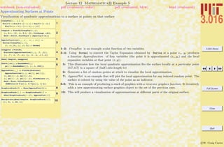
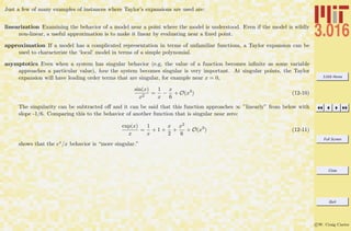
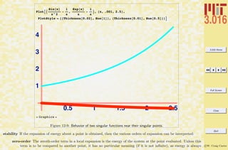
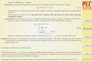
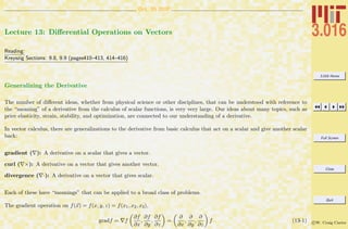
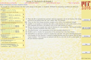
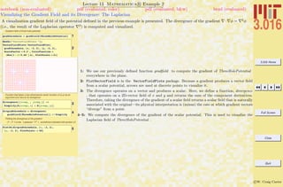
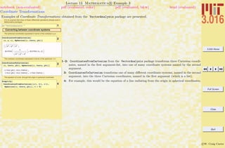
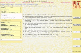
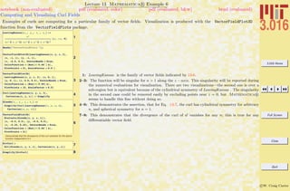
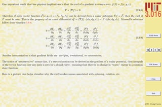
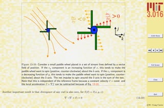
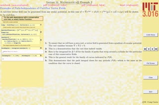
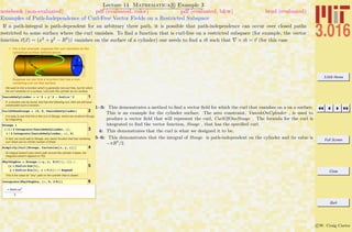
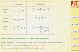
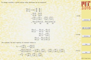
210. 3.016 Home
Full Screen
Close
Quit
c W. Craig Carter
Using the Maxwell relation, ∂S
∂P T
= − ∂V
∂T P
,
CP − CV = −T
[ ∂V
∂T P
]2
∂V
∂P T
(14-12)
which demonstrates that CP > CV because, for any stable substance, the volume is a decreasing function of pressure at
constant temperature.
. Example of a Multiple Integral: Electrostatic Potential above a Charged Region
This will be an example calculation of the spatially-dependent energy of a unit point charge in the vicinity of a charged planar
region having the shape of an equilateral triangle. The calculation superimposes the charges from each infinitesimal area by
integrating a 1/r potential from each point in space to each infinitesimal patch in the equilateral triangle The energy of a
point charge |e| due to a surface patch on the plane z = 0 of size dξdη with surface charge density σ(x, y) is:
dE(x, y, z, ξ, η) =
|e|σ(ξ, η)dξdη
r(x, y, z, ξ, η)
(14-13)
for a patch with uniform charge,
dE(x, y, z, ξ, η) =
|e|σdξdη
(x − ξ)2 + (y − η)2 + z2
(14-14)
For an equilateral triangle with sides of length one and center at the origin, the vertices can be located at (0,
√
3/2) and
(±1/2, −
√
3/6).
The integration becomes
E(x, y, z) ∝
√
3/2
−
√
3/6
√
3/2−η
η−
√
3/2
dξ
(x − ξ)2 + (y − η)2 + z2
dη (14-15)

211. 3.016 Home
Full Screen
Close
Quit
c W. Craig Carter
Lecture 14 Mathematica R Example 4
Integrals over Variable Domains
notebook (non-evaluated) pdf (evaluated, color) pdf (evaluated, b&w) html (evaluated)
This will demonstrate how Mathematica R handles multiple integrals; in particular, when the domains depend on the integration
variables. The goal is to find a function that will give the potential in the vicinity of a triangular patch with uniform charge density.
We will attempt to model the energy of ion just above one half of a
triangular capacitor. Suppose there is a uniformly charged surface (sª
charge/area=1) occupying an equilaterial triangle in the z=0 plane:
what is the energy (voltage) of a unit positive charge located at (x,y,z)
The electrical potential goes like 1
r
, therefore the potential of a unit
charge located at (x,y,z) from a small surface patch at (x,h,0) is
s dx dh
r
=
dx dh
Hx-x L2
+Hy-hL2
+z2
Therefore it remains to integrate this function over the domain hœ(0,
3
2
)
and xœ (
h
3
-
1
2
) , ( 1
2
-
h
3
))
Ÿ0
3
2
Ÿ h
3
-
1
2
1
2
-
h
3 dx dh
Hx-x L2
+Hy-hL2
+z2
„ x „ h
1
Integrate@f@x, yD, y, xD
Integrate@f@x, yD, 8y, Yi, Yf<, 8x, Xi, Xf<D
Integrate@f@x, yD,
8y, Yi, Yf<, 8x, Xi@yD, Xf@yD<D
For example,consider the difference in the following two cases:
First, we integrate over x and y using the two iterators in Integrate with
the order {y,0,1}, {x,0,y}. Tnen explicitely using two separate steps
2
Integrate@Exp@3 xD, 8y, 0, 1<, 8x, 0, y<D
interx = Integrate@Exp@3 xD, 8x, 0, y<D
Integrate@interx, 8y, 0, 1<D
Compared to
integrate over x and y using the two iterators in Integrate with the order
{x,0,y},{y,0,1}. Tnen explicitely using two separate steps
3
Integrate@Exp@3 xD, 8x, 0, y<, 8y, 0, 1<D
intery = HIntegrate@Exp@3 xD, 8y, 0, 1<DL
Integrate@intery, 8x, 0, y<D
1: These examples demonstrate that Mathematica R integrates over the last iterator which appears
in the argument-list of Integrate first: LIFI-FILI (last iterator, first integrated; first iterator, last
integrated).
2–3: Here we demonstrate the order of integration explicitly, by first integrating with two iterators, and
then integrating in two step-sequence. The methods are equivalent.

212. 3.016 Home
Full Screen
Close
Quit
c W. Craig Carter
Lecture 14 Mathematica R Example 5
Potential near a Charged and Shaped Surface Patch: Brute Force
notebook (non-evaluated) pdf (evaluated, color) pdf (evaluated, b&w) html (evaluated)
A example of a multiple integral and its numerical evaluation for the triangular charged patch.
1
TrianglePotentialNumeric@x_, y_, z_D :=
NIntegrateB1 ì Hx - xL2
+ Hy - hL2
+ z2
, :h, 0,
3 í 2>, :x, h í 3 - 1 ê 2, 1 ê 2 - h í 3 >F
2TrianglePotentialNumeric@1, 3, .01D
3Plot@TrianglePotentialNumeric@x, x, 1 ê 40D,
8x, -1, 1<D
4
cplot@h_D := cplot@hD = ContourPlot@
TrianglePotentialNumeric@x, y, hD,
8x, -1, 1<, 8y, -0.5, 1.5<, Contours Ø
Table@v, 8v, .25, 2, .25<D, ColorFunction Ø
ColorData@"TemperatureMap"D,
ColorFunctionScaling -> False,
PlotPoints Ø 11D
Timing@cplot@1 ê 10DD
5
Row@8TextCell@
"Computing ContourPlots a different
h: Progress: ", "Text"D,
ProgressIndicator@Dynamic@hD, 80, .5<D<D
cplots = Table@cplot@hD, 8h, .025, .5, .025<D;
6ListAnimate@cplotsD
1: Mathematica R can’t seem to find a closed-form solution to this integral over the triangular domain,
However, the energy can be integrated numerically. Here is a function that calls NIntegrate for a
location given by its arguments. We will call this function at different heights z. Multidimensional
integration is generally computationally expensive.
2–3: Here are examples calling the numerical function TrianglePotentialNumeric . First, the function is
evaluated at a single point; next, it is evaluated and plotted along a ◦
45-line parallel in the z = 1/40
plane.
4: The function cplot calls TrianglePotentialNumeric repeatedly at variable x and y to generate a
ContourPlot at height specified by the argument to cplot . These plots will eventually appear in an
animation, so ColorFunctionScaling is set to false so that the colors will be consistent between
frames. The Contours are set explicitly so that they are also consistent across frames. Timing
indicates that each plot consumes a large number of cpu cycles.
5: Because each frame is expensive to compute, it is not a good idea to compute them within an
animation. Here, we use Table to generate individual frames (n.b., the cplots stores its previous
calculations in memory). Because this is time consuming, we add a progress monitor that will
dynamically update as each cplot[h] is computed. We use ProgressIndicator on the argument
Dynamic[h]. Dynamic informs Mathematica R that a particular variable will be changing;
therefore the object that calls it will need to be updated.
6: We use ListAnimate on the pre-computed frames.

213. 3.016 Home
Full Screen
Close
Quit
c W. Craig Carter
Oct. 27 2006
Lecture 15: Surface Integrals and Some Related Theorems
Reading:
Kreyszig Sections: 10.4, 10.5, 10.6, 10.7 (pages439–444, 445–448, 449–458, 459–462)
Green’s Theorem for Area in Plane Relating to its Bounding Curve
Reappraise the simplest integration operation, g(x) = f(x)dx. Temporarily ignore all the tedious mechanical rules of finding
and integral and concentrate on what integration does.
Integration replaces a fairly complex process—adding up all the contributions of a function f(x)—with a clever new function
g(x) that only needs end-points to return the result of a complicated summation.
It is perhaps initially astonishing that this complex operation on the interior of the integration domain can be incorporated
merely by the domain’s endpoints. However, careful reflection provides a counterpoint to this marvel. How could it be
otherwise? The function f(x) is specified and there are no surprises lurking along the x-axis that will trip up dx as it marches
merrily along between the endpoints. All the facts are laid out and they willingly submit to the process their preordination
by g(x) by virtue of the endpoints.8
The idea naturally translates to higher dimensional integrals and these are the basis for Green’s theorem in the plane, Stoke’s
theorem, and Gauss (divergence) theorem. Here is the idea:
8
I do hope you are amused by the evangelistic tone. I am a bit punchy from working non-stop on these lectures and wondering if anyone is really
reading these notes. Sigh.

214. 3.016 Home
Full Screen
Close
Quit
c W. Craig Carter
x
y
z
Figure 15-11: An irregular region on a plane surrounded by a closed curve. Once the closed
curve (the edge of region) is specified, the area inside it is already determined. This is the
simplest case as the area is the integral of the function f = 1 over dxdy. If some other
function, f(x, y), were specified on the plane, then its integral is also determined by summing
the contributions along the boundary. This is a generalization g(x) = f(x)dx and the basis
behind Green’s theorem in the plane.
The analog of the “Fundamental Theorem of Differential and Integral Calculus”9 for a region R bounded in a plane with
normal ˆk that is bounded by a curve ∂R is:
R
( × F) · ˆkdxdy =
∂R
F · dr (15-1)
The following figure motivates Green’s theorem in the plane:
9
This is the theorem that implies the integral of a derivative of a function is the function itself (up to a constant).

215. 3.016 Home
Full Screen
Close
Quit
c W. Craig Carter
i
k
j
!vy
!x >0
!vx
!y <0
Figure 15-12: Illustration of how a vector valued function in a planar domain ”spills out” of
domain by evaluating the curl everywhere in the domain. Within the domain, the rotational
flow ( × F) from one cell moves into its neighbors; however, at the edges the local rotation
is a net loss or gain. The local net loss or gain is F · (dx, dy).
The generalization of this idea to a surface ∂B bounding a domain B results in Stokes’ theorem, which will be discussed later.
In the following example, Green’s theorem in the plane is used to simplify the integration to find the potential above a
triangular path that was evaluated in a previous example. The result will be a considerable increase of efficiency of the
numerical integration because the two-dimensional area integral over the interior of a triangle is reduced to a path integral
over its sides.
The objective is to turn the integral for the potential
E(x, y, z) =
R
dξdη
(x − ξ)2 + (y − η)2 + z2
(15-2)
into a path integral using Green’s theorem in the x–y plane:
R
∂F2
∂x
−
∂F1
∂y
dxdy =
∂R
(F1dx + F2dy) (15-3)

216. 3.016 Home
Full Screen
Close
Quit
c W. Craig Carter
To find the vector function F = (F1, F2) which matches the integral in question, set F2 = 0 and integrate to find F1 via
dη
(x − ξ)2 + (y − η)2 + z2
(15-4)

217. 3.016 Home
Full Screen
Close
Quit
c W. Craig Carter
Lecture 15 Mathematica R Example 1
Converting an area-integral over a variable domain into a path-integral over its boundary
notebook (non-evaluated) pdf (evaluated, color) pdf (evaluated, b&w) html (evaluated)
We reproduce the example from Lecture 14 where the potential was calculated in the vicinity of a triangular patch, but with much
improved accuracy and speed. The previous example’s two dimensional numerical integration which requires O(N2
) calculations into
a path integration around the boundary which requires O(N) evaluations for the same accuracy. The path of integration must be
determined (i.e., (x(t), y(t))) and then the integration is obtained via (dx, dy) = (x dt, y dt).
Suppose there is a uniformly charged surface (sªcharge/area=1)
occupying an equilaterial triangle in the z=0 plane:
1
F1@x_, y_ , z_D =
-IntegrateB
1
Hx - xL2
+ Hy - hL2
+ z2
, hF
The third (horizontal) boundary of the triangle patch looks like the easiest,
let's see if an integral can be found over that patch:
2
Bottomside =
F1@x, y, zD ê. :x Ø t -
1
2
, h Ø 0> êê Simplify
3
NEside = F1@x, y, zD ê.
:x Ø
1 - t
2
, h Ø
3 t
2
> êê Simplify
4
NWside = F1@x, y, zD ê.
:x Ø
-t
2
, h Ø
3 H1 - tL
2
> êê Simplify
5
integrand =
SimplifyB
-HNEside + NWsideL
2
+ BottomsideF
1: We use Green’s theorem in the plane to turn our original integral
ZZ
triangle
region
„
∂F2
∂η
−
∂F1
∂ξ
«
dξdη = φ(x, y, z)
=
ZZ
dηdξ
r(x − ξ, y − η, z)
=
I
triangle
perimeter
F · ds
A closed form for F1 (as indicated in Equation 15-4) is obtained with Integrate.
2: The bottom part of the triangle can be written as the curve: (ζ(t), η(t)) = (t − 1
2
, 0) for 0 < t < 1;
the integrand over that side is obtained by suitable replacement.
3–4: The remaining two legs of the triangle can be written similarly as: ((1 − t)/2,
√
3t/2) and
(−t/2,
√
3(1 − t)/2).
5: This is the integrand for the entire triangle to be integrated over 0 < t < 1. Note, as t goes from 0
to 1, each leg of the triangle is traversed; this integrand sums all three contributions.

218. 3.016 Home
Full Screen
Close
Quit
c W. Craig Carter
Lecture 15 Mathematica R Example 2
Faster and More Accurate Numerical Integration by Using Green’s Theorem.
notebook (non-evaluated) pdf (evaluated, color) pdf (evaluated, b&w) html (evaluated)
Continuing the example above, we are now able to find the potential over a triangular patch with uniform charge density, with a
one-dimensional numerical integration, instead of the two-dimensional numerical integration in the last lecture.
Doing the same integral as in the previous lecture numerically, but this
time over the boundary of the triangle instead of the triangle area.
1
Pot@X_, Y_, Z_D := NIntegrate@Evaluate@
integrand ê. 8x Ø X, y Ø Y, z Ø Z<D, 8t, 0, 1<D
We will create contourplots (level sets of constant potential) at as a
function of different heights. We check the timing of the computation to
compare to method in the last lecture.
2
ncplot@h_D :=
ncplot@hD = ContourPlot@Pot@a, b, hD,
8a, -1, 1<, 8b, -.5, 1.5<, Contours Ø
Table@v, 8v, .25, 2, .25<D, ColorFunction Ø
ColorData@"TemperatureMap"D,
ColorFunctionScaling -> False,
PlotPoints Ø 11 , ImageSize Ø 896, 72<D
Timing@ncplot@.05DD
3
Row@8TextCell@
"Computing ContourPlots a different
h: Progress: ", "Text"D,
ProgressIndicator@Dynamic@hD, 80, .5<D<D
ncplots = Table@ncplot@hD,
8h, .025, .5, .025<D;
4ListAnimate@ncplotsD
1: There is no free lunch—the closed form of the integral is either unknown or takes too long to
compute. However, NIntegrate is much more efficient because the problem has been reduced to a
single integral instead of the double integral in the previous example.
2: A ContourPlot showing the level sets of the scalar potential field at a particular height h is obtained
by a single call to the function ncplot . Timing shows that a speed-up factor of two is obtained for
a single plot.
3: Here, we calculate a sequence of contour plots and store them for subsequent animation. Because
this calculation takes a while to finish, we add a ProgressIndicator.
4: This is an animation for the potential in a plane as we increase the height of the plane above the
triangular patch.

219. 3.016 Home
Full Screen
Close
Quit
c W. Craig Carter
Representations of Surfaces
Integration over the plane z = 0 in the form of f(x, y)dxdy introduces surface integration—over a planar surface—as a
straightforward extension to integration along a line. Just as integration over a line was generalized to integration over a
curve by introducing two or three variables that depend on a single variable (e.g., (x(t), y(t), z(t))), a surface integral can be
conceived as introducing three (or more) variables that depend on two parameters (i.e., (x(u, v), y(u, v), z(u, v))).
However, there are different ways to formulate representations of surfaces:
Surfaces and interfaces play fundamental roles in materials science and engineering. Unfortunately, the mathematics of
surfaces and interfaces frequently presents a hurdle to materials scientists and engineering. The concepts in surface analysis
can be mastered with a little effort, but there is no escaping the fact that the algebra is tedious and the resulting equations
are onerous. Symbolic algebra and numerical analysis of surface alleviates much of the burden.
Most of the practical concepts derive from a second-order Taylor expansion of a surface near a point. The first-order terms
define a tangent plane; the tangent plane determines the surface normal. The second-order terms in the Taylor expansion form
a matrix and a quadratic form that can be used to formulate an expression for curvature. The eigenvalues of the second-order
matrix are of fundamental importance.
The Taylor expansion about a particular point on the surface takes a particularly simple form if the origin of the coordinate
system is located at the point and the z-axis is taken along the surface normal as illustrated in the following figure.

220. 3.016 Home
Full Screen
Close
Quit
c W. Craig Carter
xegn
yegn
z
n
ru
rv
Figure 15-13: Parabolic approximation to a surface and local eigenframe. The surface
on the left is a second-order approximation of a surface at the point where the coordinate axes
are drawn. The surface has a local normal at that point which is related to the cross product
of the two tangents of the coordinate curves that cross at the that point. The three directions
define a coordinate system. The coordinate system can be translated so that the origin lies at
the point where the surface is expanded and rotated so that the normal ˆn coincides with the
z-axis as in the right hand curve.
In this coordinate system, the Taylor expansion of z = f(x, y) must be of the form
∆z = 0dx + 0dy +
1
2
(dx, dy)
∂2f
∂x2
∂2f
∂x∂y
∂2f
∂x∂y
∂2f
∂y2
dx
dy
If this coordinate system is rotated about the z-axis into its eigenframe where the off-diagonal components vanish, then the
two eigenvalues represent the maximum and minimum curvatures. The sum of the eigenvalues is invariant to transformations
and the sum is known as the mean curvature of the surface. The product of the eigenvalues is also invariant—this quantity
is known as the Gaussian curvature.

221. 3.016 Home
Full Screen
Close
Quit
c W. Craig Carter
The method in the figure suggests a method to calculate the normals and curvatures for a surface. Those results are tabulated
below.
Level Set Surfaces: Tangent Plane, Surface Normal, and Curvature
F(x, y, z) = const
Tangent Plane (x = (x, y, z), ξ = (ξ, η, ζ))
F · (ξ − x) or
∂F
∂x
(ξ − x) +
∂F
∂y
(η − y) +
∂F
∂z
(ζ − z)
Normal
ξ − x
∂F
∂x
=
η − y
∂F
∂y
=
ζ − z
∂F
∂z
Mean Curvature
· F
F or
2
6
6
4
∂2F
∂y2 + ∂2F
∂z2 (∂F
∂x )2 + ∂2F
∂z2 + ∂2F
∂x2 (∂F
∂y )2 + ∂2F
∂x2 + ∂2F
∂y2 (∂F
∂z )2
−2 ∂F
∂x
∂F
∂y
∂2F
∂x∂y + ∂F
∂y
∂F
∂z
∂2F
∂y∂z + ∂F
∂z
∂F
∂x
∂2F
∂z∂x
3
7
7
5
“
∂F
∂x
2
+ ∂F
∂y
2
+ ∂F
∂z
2
”3/2

222. 3.016 Home
Full Screen
Close
Quit
c W. Craig Carter
Parametric Surfaces: Tangent Plane, Surface Normal, and Curvature
x = (p(u, v), q(u, v), s(u, v)) or x = p(u, v)y = q(u, v)z = s(u, v)
Tangent Plane (x = (x, y, z), ξ = (ξ, η, ζ))
(ξ − x) · (
dx
du
×
dx
dv
) det


ξ − x η − y ζ − z
∂p
∂u
∂q
∂u
∂s
∂u
∂p
∂v
∂q
∂v
∂s
∂v

 = 0
Normal
ξ − x
∂(q,s)
∂(u,v)
=
η − y
∂(s,p)
∂(u,v)
=
ζ − z
∂(p,q)
∂(u,v)
Mean Curvature
dx
du · dx
du
dx
du × dx
dv · d2x
dv2 − 2 dx
du · dx
dv
dx
du × dx
dv · d2x
dudv + dx
dv · dx
dv
dx
du × dx
dv · d2x
du2
dx
du × dx
dv · dx
du × dx
dv
3/2

223. 3.016 Home
Full Screen
Close
Quit
c W. Craig Carter
Graph Surfaces: Tangent Plane, Surface Normal, and Curvature
z = f(x, y)
Tangent Plane (x = (x, y, z), ξ = (ξ, η, ζ))
∂f
∂x
(ξ − x) +
∂f
∂y
(η − y) = (ζ − z)
Normal
ξ − x
∂f
∂x
=
η − y
∂f
∂y
=
ζ − z
−1
Mean Curvature
(1 + ∂f
∂x
2
)∂2f
∂y2 − 2∂f
∂x
∂f
∂y
∂2f
∂x∂y + (1 + ∂f
∂y
2
)∂2f
∂x2
1 + ∂f
∂x
2
+ ∂f
∂y
2

224. 3.016 Home
Full Screen
Close
Quit
c W. Craig Carter
Lecture 15 Mathematica R Example 3
Representations of Surfaces: Graphs z = f(x, y) (part 1)
notebook (non-evaluated) pdf (evaluated, color) pdf (evaluated, b&w) html (evaluated)
Visualization examples of surfaces represented by the graph z = f(x, y); Examples of the use of MeshFunctions and ColorFunction
to visualize various surface properties are given.
1
GraphFunction@x_, y_D :=
Hx - yL Hx + yL ë I1 + Hx + yL2
M
assump = 8x œ Reals, y œ Reals<
2plotdefault = Plot3D@GraphFunction@x, yD,
8x, -3, 3<, 8y, -3, 3<, PlotLabel Ø "Default"D
3
plotlevels =
Plot3D@GraphFunction@x, yD, 8x, -3, 3<,
8y, -3, 3<, MeshFunctions Ø H Ò3 &L,
ColorFunction Ø "Rainbow",
PlotLabel Ø "Constant Heights"D
4
angle@x_D := HHPi ê 2 + ArcTan@xDL ê PiL
angle@x_, y_D := HHPi ê 2 + ArcTan@x, yDL ê PiL
5
plotcircles = Plot3D@
GraphFunction@x, yD, 8x, -3, 3<, 8y, -3, 3<,
MeshFunctions Ø HSqrt@Ò1^2 + Ò2^2D &L,
ColorFunction -> HHue@angle@Ò1, Ò2D * 0.5D &L,
ColorFunctionScaling Ø False,
PlotLabel Ø "Cylindrical Coordinates"D
6
CurvatureOfGraph@f_, x_, y_D :=
FullSimplify@Module@
8dfdx = D@f@x, yD, xD, dfdy = D@f@x, yD, yD,
d2fdx2 = D@f@x, yD, 8x, 2<D,
d2fdy2 = D@f@x, yD, 8y, 2<D,
d2fdxdy = D@f@x, yD, x, yD< ,
Return@HH1 + dfdx^2L d2fdx2 - 2 dfdx
dfdy d2fdxdy + H1 + dfdy^2L d2fdy2L ê
Sqrt@1 + dfdx^2 + dfdy^2DDD,
Assumptions Ø assumpD
7CurvFunc = Function@8x, y<, Evaluate@
CurvatureOfGraph@GraphFunction, x, yDDD
1: We will use GraphFunction as an example to show different ways to visualize a graph over an area.
2: Plot3D is used to plot GraphFunction with default settings.
3: Here is an example of using MeshFunctions to draw lines at constant altitude (i.e, constant values
of f(x, y))
4: This function, angle , which maps angles to the range (0, 1) will be useful for visualization examples
below (e.g., 5 and the following sections 2).
5: This will help visualize a cylindrical- in addition to the Cartesian-coordinate system. The
MeshFunctions option is used to plot concentric circles; ColorFunction illustrates the angular
coordinate, θ, with Hue.
6: Our goal is to visualize curvature on top of the graph. This is a somewhat advanced example. Here
we construct a function (CurvatureOfGraph ) that computes the curvature H(x, y) of an f(x, y), and
uses FullSimplify with assumptions that the coordinate are real numbers.
7: Here we use Function to create a symbol representing a function of two variables for the particular
instance of the curvature of f =GraphFunction . Evaluate is used in the definition to ensure that
the curvature computation is performed only once.

225. 3.016 Home
Full Screen
Close
Quit
c W. Craig Carter
Lecture 15 Mathematica R Example 4
Representations of Surfaces: Graphs z = f(x, y) (part 2)
notebook (non-evaluated) pdf (evaluated, color) pdf (evaluated, b&w) html (evaluated)
We continue the example by visualizing the curvature and the inclination of the graph.
1
dfdx = Function@8x, y<, Evaluate@
FullSimplify@D@GraphFunction@x, yD, xD,
Assumptions Ø assumpDDD
dfdy = Function@8x, y<, Evaluate@
FullSimplify@D@GraphFunction@x, yD, yD,
Assumptions Ø assumpDDD
This is the surface with lines of constant curvature superimposed, and
with colors associated with the local normal.
2
plotcurvature = Plot3D@
GraphFunction@x, yD, 8x, -3, 3<, 8y, 3, -3<,
MeshFunctions Ø HCurvFunc@Ò1, Ò2D &L,
MeshStyle Ø Thick, PlotLabel Ø
"CurvaturesHlevel setsL and NormalsHcolor
variationL", ColorFunction Ø
HGlow@RGBColor@angle@dfdx@Ò1, Ò2DD,
angle@dfdy@Ò1, Ò2DD, 0.75DD &L,
ColorFunctionScaling Ø False,
Lighting Ø NoneD
Visualizing all the examples together.
3
GraphicsGrid@88plotdefault, plotlevels<,
8plotcircles, plotcurvature<<,
ImageSize Ø 2 872, 72<D
1: Two more symbols for functions of two arguments are created. Each represents a the slope of the
tangent plane in the directions of the coordinate axes.
2: Plot3D is used to illustrate the local tangent-plane with ColorFunction which points to a red-scale
for the surface slope in the x-direction and a blue-scale for the y-slope. We use Glow with Lighting
set to none.
3: Finally, we use GraphicsGrid to illustrate the four graphic-examples together.

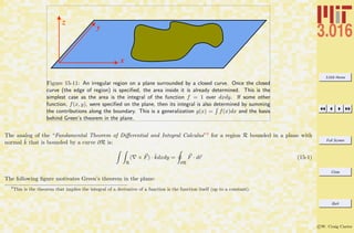
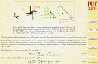
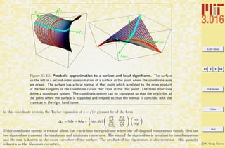
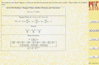
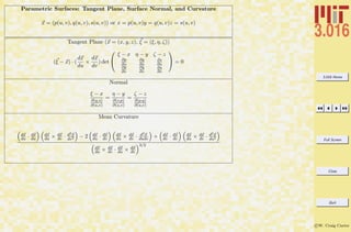
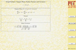
226. 3.016 Home
Full Screen
Close
Quit
c W. Craig Carter
Lecture 15 Mathematica R Example 5
A Frivolous Example for Graphs z = f(x, y): Floating Pixels from Images in 3D
notebook (non-evaluated) pdf (evaluated, color) pdf (evaluated, b&w) html (evaluated)
We demonstrate how to read a grey-scale image into Mathematica R , and then use the pixel brightness values to displace the images
according to z = brightness(x, y).
1
MinMax@alist_ListD :=
Module@8flatlist = Flatten@alistD<,
Return@8Min@flatlistD, Max@flatlistD<DD
mug = Import@
"http:êêpruffle.mit.eduê~ccarterêch_face
_framesêCarter_2000_verysmall.png"D;
ProgressIndicator@Dynamic@iD, 81, 64<D
vp@i_D := 8.1 Sin@Hi - 1L Pi ê 31D,
Sin@Hi - 1L 2 Pi ê 31D, 2 Cos@2 Hi - 1L Pi ê 63D<;
minmax = MinMax@mug@@1, 1DDD;
Table@mugshot@iD =
ListPlot3D@mug@@1, 1DD, MeshStyle -> None,
Mesh Ø None, InterpolationOrder Ø 0,
ColorFunction Ø "GreenBrownTerrain",
Axes Ø False, ViewPoint Ø vp@iD,
PlotRange Ø minmax,
ImageSize Ø Full,
SphericalRegion Ø TrueD;, 8i, 1, 64<D;
Manipulate@mugshot@frameD, 8frame, 1, 64, 1<D
frame
1: We first construct a function that will pick out the largest and smallest numbers in a list, and this
will allow us to set PlotRange between the darkest and brightest pixels. (This function should
probably check to ensure that the list contains only numeric entries, so that Max and Min return
sensible results.) We will create a 3D rendering of pixels and “fly” through it. The function vp will
provide the “orbit” for our flight through the pixels.
Table is used to create Graphics3D objects from different viewpoints for subsequent animation.
Each graphics object is created with ListPlot3D with an array of pixel values for the first argument
(mug[[1,1]]). Using InterpolationOrder set to zero implies that the plot’s discrete values will not
be continuously connected (i.e., the pixels are not “warped” to ensure continuity).
I used a modified version of this example to add an animation to my homepage

227. 3.016 Home
Full Screen
Close
Quit
c W. Craig Carter
Lecture 15 Mathematica R Example 6
A Frivolous Example for Graphs z = f(x, y): Creating and Animating Surfaces from Image Sequences
notebook (non-evaluated) pdf (evaluated, color) pdf (evaluated, b&w) html (evaluated)
We read in a sequence of images and use their pixel values to create an interpolation function for a surface z = brightness(x, y). Plot3D
calls the interpolation function produces a 3D animation from a 2D one.
1
Table@chface@readD = Import@
"http:êêpruffle.mit.eduê~ccarterêch_face
_framesêch_face." <>
ToString@100 + read - 1D <> ".png"D;
facedata@readD = ListInterpolation@
chface@readD@@1, 1DD, 880, 1<, 80, 1<<D;
If@read ã 1, minmax =
MinMax@chface@readD@@1, 1DDD;, minmax =
MinMax@8minmax, chface@readD@@1, 1DD<DD;,
8read, 1, 28, 1<D;
pface@i_D := Plot3D@facedata@iD@x, yD,
8y, 0, 1<, 8x, 0, 1<, PlotRange Ø minmax,
ColorFunction Ø "GreenBrownTerrain",
Mesh Ø False, Axes Ø False,
ViewPoint Ø 8-0.25, -2, 5<, ImageSize Ø AllD
ListAnimate@Table@pface@gcompD,
8gcomp, 1, 28, 1<D, DefaultDuration Ø 10D
1: Table is used to iteratively read images that were created from a typical web-animation. (I am
working on a way to do this directly from a single image file with multiple frames (with color), but
haven’t finished yet. ListInterpolation is used to create a continuous function of x and y in the
domain 0 < |x|&|y| < 1. The height of the function corresponds to the brightness of the pixel. The
function pface [i] produces a Graphics3D object for each frame in the animation. ListAnimate
produces the animation from the image-functions.

228. 3.016 Home
Full Screen
Close
Quit
c W. Craig Carter
Lecture 15 Mathematica R Example 7
Representations of Surfaces: Parametric Surfaces x(u, v)
notebook (non-evaluated) pdf (evaluated, color) pdf (evaluated, b&w) html (evaluated)
Visualization techniques for surfaces of the form (x(u, v), y(u, v), z(u, v)) are presented.
1
SurfaceParametric@u_, v_D := 8Cos@uD v,
u Cos@u + vD, Cos@uD ê H.1 + Cos@uD^2L<
2
ParametricPlot3D@
Evaluate@SurfaceParametric@u, vDD,
8u, -2, 2<, 8v, -2, 2<D
Using Manipulate, we can vary the boundary domain, and provide a more
intuitive way to understand this complicated surface.
3
evolution = Table@ParametricPlot3D@
Evaluate@SurfaceParametric@u, vDD,
8u, -ep, ep<, 8v, -ep, ep<, PlotRange Ø
88-4, 4<, 8-4, 4<, 8-4, 4<<, PlotPoints Ø
81 + Round@ep ê .125D, 1 + Round@ep ê .125D<,
ImageSize Ø FullD, 8ep, .125, 4.25, .125<D;
ListAnimate@evolution, ImageSize Ø FullD
1–2: Using ParametricPlot3D to visualize a surface of the form (x(u, v), y(u, v), z(u, v)) given by Sur-
faceParametric . The lines of constant u and v generate the “square mesh” of the approximation to
the surface. Each line on the surface is of the form: r1(u) = (x(u, v = const), y(u, v = const), z(u, v =
const)) and r2(v) = (x(u = const, v), y(u = const, v), z(u = const, v)). The set of all crossing lines
r1(u) and r2(v) is the surface. Each little “square” surface patch provides a convenient way to define
the local surface normal—because both the vectors dr1/du and dr2/dv are tangent to the surface,
their cross-product is either an inward-pointing normal or outward-pointing normal.
3: The nature of parametric surfaces are typically much more complicated than for graphs. Because the
surface often folds over and through itself, it is difficult to comprehend its shape. For this case, it is
useful to visualize the evolution of the surface as the domain of (u, v) increases. Here we use Table
to iteratively increase the size of the domain, and then use ListAnimate to visualize its evolution.

229. 3.016 Home
Full Screen
Close
Quit
c W. Craig Carter
Lecture 15 Mathematica R Example 8
Representations of Surfaces: Level Sets constant = f(x, y, z)
notebook (non-evaluated) pdf (evaluated, color) pdf (evaluated, b&w) html (evaluated)
Visualization examples of surfaces represented their level sets constant = F(x, y, z) are presented. This type of surface representation
is particularly convenient when surfaces are disconnected, or merge during an evolution. Level sets are used extensively in phase field
models of microstructural evolution.
1ConstFunction = x2
- 4 x y + y2
+ z2
2ContourPlot3D@ConstFunction, 8x, -1, 1<,
8y, -1, 1<, 8z, -1, 1<, Contours Ø 82.5<D
The following statements produce contour plots of the same function,
using two different methods for colorizing the surfaces...
3cpa = ContourPlot3D@ConstFunction, 8x, -3, 3<,
8y, -3, 3<, 8z, -3, 3<, Contours Ø 80, 2, 8<D
4
cpb = ContourPlot3D@ConstFunction,
8x, -3, 3<, 8y, -3, 3<, 8z, -3, 3<,
Contours Ø 80, 2, 8<, ContourStyle Ø 8
Directive@Pink, Opacity@0.8DD,
Directive@Yellow, Opacity@0.8DD,
Directive@Orange, Opacity@0.8DD<D
5
Manipulate@
ContourPlot3D@ConstFunction, 8x, -3, 3<,
8y, -3, 3<, 8z, -3, 3<, Contours -> 8i<,
ImageSize Ø FullD, 8i, -2, 10, .25<D
1: ConstFunction will be used for the following visualization examples.
1–2: A contour in two-dimensions is a curve; we have seen examples of such curves with ContourPlot.
A contour in three-dimensions is a surface and we will use ContourPlot3D to visualize the level set
formulation of a surface constant = F(x, y, z) given by ConstFunction . Here, we explicitly specify
those x, y, and z for which x2
− 4xy + y2
+ z2
= 2.5.
3: Here is an example of specifying three different level sets by passing several Contours to
ContourPlot3D. It is difficult to distinguish which surface belongs to a particular level set.
4: The surfaces can be distinguished from one another with by giving each a different graphics
Directive its own color. Setting Opacity to a value less than one helps eliminate the ‘hidden
surface’ problem.
5: The evolution of level sets can be visualized with Manipulate by varying the value that is passed to
Contours. It is apparent why this surface representation is useful when surfaces undergo topological
changes. It may be helpful to consider these changes as a higher dimensional effect: consider t =
f(x, y, z) as a graph ‘over’ 3D region, or a four-dimensional surface. As a lower dimensional example
(i.e., t = f(x, y)), consider the curves that develop as a torus (ummmm doughnut) is slice sequentially
from one side. Initially the perimeter is an single closed elongated loop, which eventually begins to
pinch in the middle and then break into isolated curves.

230. 3.016 Home
Full Screen
Close
Quit
c W. Craig Carter
Integration over Surfaces
Integration of a function over a surface is a straightforward generalization of f(x, y)dxdy = f(x, y)dA. The set of all
little rectangles dxdy defines a planar surface. A non-planar surface x(u, v) is composed of a set of little parallelogram patches
with sides given by the infinitesimal vectors
rudu =
∂x
∂u
du
rvdu =
∂x
∂v
dv
(15-5)
Because the two vectors ru and rv are not necessarily perpendicular, their cross-product is needed to determine the magnitude
of the area in the parallelogram:
dA = ru × rv dudv (15-6)
and the integral of some scalar function, g(u, v) = g(x(u, v), y(u, v)) = g(x(u, v)), on the surface is
g(u, v)dA = g(u, v) ru × rv dudv (15-7)
However, the operation of taking the norm in the definition of the surface patch dA indicates that some information is getting
lost—this is the local normal orientation of the surface. There are two choices for a normal (inward or outward).
When calculating some quantity that does not have vector nature, only the magnitude of the function over the area matters
(as in Eq. 15-7). However, when calculating a vector quantity, such as the flow through a surface, or the total force applied
to a surface, the surface orientation matters and it makes sense to consider the surface patch as a vector quantity:
A(u, v) = A ˆn(u, v) = Aˆn(u, v)
dA = ru × rv
(15-8)
where ˆn(u, v) is the local surface unit normal at x(u, v).

231. 3.016 Home
Full Screen
Close
Quit
c W. Craig Carter
Lecture 15 Mathematica R Example 9
Example of an Integral over a Parametric Surface
notebook (non-evaluated) pdf (evaluated, color) pdf (evaluated, b&w) html (evaluated)
The surface energy of single crystals often depends on the surface orientation. This is especially the case for materials that have covalent
and/or ionic bonds. To find the total surface energy of such a single crystal, one has to integrate an orientation-dependent surface energy,
γ(ˆn), over the surface of a body. This example compares the total energy of such an anisotropic surface energy integrated over a sphere
and a cube that enclose the same volume.
1
sphere@u_ , v_ D :=
R 8Cos@vD Cos@uD , Cos@vD Sin@uD , Sin@vD<
2
Ru@u_ , v_D = D@sphere@u, vD, uD êê Simplify
Rv@u_ , v_D = D@sphere@u, vD, vD êê Simplify
3
Needs@"VectorAnalysis`"D
NormalVector@u_ , v_ D =
CrossProduct@Ru@u, vD, Rv@u, vDD êê Simplify
NormalMag = FullSimplify@
Norm@NormalVector@u, vDD, Assumptions Ø
8R ¥ 0, 0 § u § 2 p, -p ê 2 < v < p ê 2<D
UnitNormal@u_, v_D =
NormalVector@u, vD ê NormalMag
4
SurfaceTension@nvec_D :=
1 + gamma111 * nvec@@1DD2
nvec@@2DD2
nvec@@3DD2
5
SphericalPlot3D@
SurfaceTension@UnitNormal@u, vDD ê.
gamma111 Ø 12,
8u, 0, 2 Pi<, 8v, -Pi ê 2, Pi ê 2<D
6
SphereEnergy = Integrate@Integrate@
SurfaceTension@UnitNormal@u, vDD Cos@vD,
8u, 0, 2 p<D, 8v, -p ê 2, p ê 2<D
7CubeSide = H4 p ê 3L^H1 ê 3L
8
CubeEnergy =
6 I CubeSide2
SurfaceTension@81, 0, 0<DM
9
EqualEnergies =
Solve@CubeEnergy ã SphereEnergy,
gamma111D êê Flatten
10N@gamma111 ê. EqualEnergiesD
1: This is the parametric equation of the sphere in terms of longitude v ∈ (0, 2π) and latitude u ∈
(−π/2, π/2).
2: Calculate the tangent plane vectors ru and rv
3: Using CrossProduct from the VectorAnalysis package to calculate a vector that is normal to the
surface, ru × rv, for subsequent use in the surface integral. Using Norm to find the magnitude of
the local normal, we can produce a function to return the unit normal vector ˆn, UnitNormal , as a
function of the surface parameters.
4: This is just an example of a γ(ˆn) that depends on direction that will be used for purposes of
illustration.
5: Using SphericalPlot3D, the form of SurfaceTension for the particular choice of γ111 = 12 is
visualized.
6: Using the result from |ru × rv|, the total surface energy of a spherical body of radius R = 1 is
computed by integrating γˆn over the entire surface.
7–8: This would be the energy of a cubical body with the same volume as the sphere with unit radius.
The cube is oriented so that its faces are normal to 100 .
9–10: This calculation is not very meaningful, but it is the value of the surface anisotropy factor γ111 such
that the cube and sphere have the same total surface energy. The total-surface-energy minimizing
shape for a fixed volume is calculated using the Wulff theorem.

232. 3.016 Home
Full Screen
Close
Quit
c W. Craig Carter
Oct. 29 2007
Lecture 16: Integral Theorems
Reading:
Kreyszig Sections: 10.8, 10.9 (pages463–467, 468–473)
Higher-dimensional Integrals
The fundamental theorem of calculus was generalized in a previous lecture from an integral over a single variable to an
integration over a region in the plane. Specifically, for generalizing to Green’s theorem in the plane, a vector derivative of a
function integrated over a line and evaluated at its endpoints was generalized to a vector derivative of a function integrated
over the plane.
x
y
z
Figure 16-14: Illustrating how Green’s theorem in the plane works. If a known vector function
is integrated over a region in the plane then that integral should only depend on the bounding
curve of that region.

233. 3.016 Home
Full Screen
Close
Quit
c W. Craig Carter
x
y
z
Figure 16-15: Illustration of a generalization to the Green’s theorem in the plane: Suppose
there is a bowl of a known shape submerged in a fluid with a trapped bubble. The bubble is
bounded by two different surfaces, the bowl down to z = 0 and the planar liquid surface at that
height. Integrating the function VB
dV over the bubble gives its volume. The volume must
also be equal to an integral ∂VB
zdxdy over the (oriented) surface of the liquid. However,
the volume of bubble can be determined from only the curve defined by the intersection of the
bowl and the planar liquid surface; so the volume must also be equal to C(some function)ds.
The Divergence Theorem
Suppose there is “stuff” flowing from place to place in three dimensions.

234. 3.016 Home
Full Screen
Close
Quit
c W. Craig Carter
z
y
x
AL AB
Figure 16-16: Illustration of a vector “flow field” J near a point in three dimensional space.
If each vector represents the rate of “stuff” flowing per unit area of a plane that is normal to
the direction of flow, then the dot product of the flow field integrated over a planar oriented
area A is the rate of “stuff” flowing through that plane. For example, consider the two areas
indicated with purple (or dashed) lines. The rate of “stuff” flowing through those regions is
J · AB = J · ˆkAB and J · AL = J · ˆkAL.
If there are no sources or sinks that create or destroy stuff inside a small box surrounding a point, then the change in the
amount of stuff in the volume of the box must be related to some integral over the box’s surface:
d
dt
(amount of stuff in box) =
d
dt box
(
amount of stuff
volume
)dV
=
box
d
dt
(
amount of stuff
volume
)dV
=
box
(some scalar function related to J)dV
= box
surface
J · dA
(16-1)

235. 3.016 Home
Full Screen
Close
Quit
c W. Craig Carter
J3( x=0; y=0; z=!z
2 )
J3( x=0; y=0; z=!!z
2 )
J2( x=0; y=!!y
2 ; z=0)
J2( x=0; y=!y
2 ; z=0)
J1( x=!!x
2 ; y=0; z=0)
J1( x=!x
2 ; y=0; z=0)
Figure 16-17: Integration of a vector function near a point and its relation to the change in
that vector function. The rate of change of stuff is the integral of flux over the outside—and
in the limit as the box size goes to zero, the rate of change of the amount of stuff is related to
the sum of derivatives of the flux components at that point.
To relate the rate at which “stuff M” is flowing into a small box of volume δV = dxdydz located at (x, y, z) due to a flux J,
note that the amount that M changes in a time ∆t is:
∆M(δV ) = (M flowing out of δV ) − (M flowing in δV )
= J(x − dx
2 )ˆidydz− J(x + dx
2 ) ·ˆidydz
+ J(y − dy
2 )ˆjdzdx− J(y + dy
2 ) · ˆjdzdx
+ J(z − dz
2 )ˆkdxdy− J(z + dz
2 ) · ˆkdxdy
∆t
= −(
∂Jx
∂x
+
∂Jy
∂y
+
∂Jz
∂z
)δV ∆t + O(dx4
)
(16-2)

236. 3.016 Home
Full Screen
Close
Quit
c W. Craig Carter
If C(x, y, z) = M(δV )/δV is the concentration (i.e., stuff per volume) at (x, y, z), then in the limit of small volumes and short
times:
∂C
∂t
= −(
∂Jx
∂x
+
∂Jy
∂y
+
∂Jz
∂z
) = − · J = −divJ (16-3)
For an arbitrary closed volume V bounded by an oriented surface ∂V :
dM
dt
=
d
dt V
CdV =
V
∂C
∂t
dV = −
V
· JdV = −
∂V
J · dA (16-4)
The last equality
V
· JdV =
∂V
J · dA (16-5)
is called the Gauss or the divergence theorem.

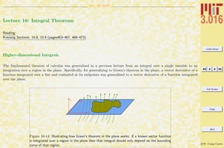
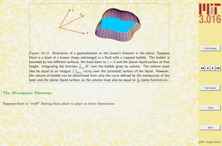
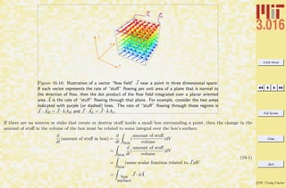
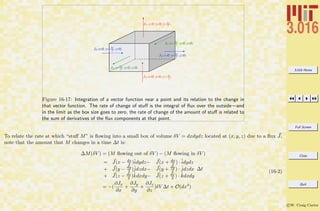
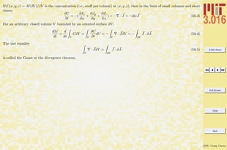
237. 3.016 Home
Full Screen
Close
Quit
c W. Craig Carter
Lecture 16 Mathematica R Example 1
London Dispersion Potential due to a Finite Body
notebook (non-evaluated) pdf (evaluated, color) pdf (evaluated, b&w) html (evaluated)
If the London interaction (i.e., energy between two induced dipoles) can be treated as a 1/r6
potential, then the potential due to a
volume is an integration over each point in the volume and and arbitrary point in space. This calculation will be made much more
efficient by turning the volume integral into a surface integral by using the divergence theorem.
Numerical integration is a cpu-time-consuming numerical procedure. If
there is a way to reduce the dimensionality of the integration, then we
can reap rewards for our cleverness. One trick is to use the divergence
theorem to push the integration over a volume, to an integration over a
surface. For example, we could use the divergence theorem:
ŸŸŸ volume “· P dV = ŸŸ surfaceP ÿd A
For a 1/r6
potential , we must find a vector potential P such that “· P =
-1/|r
”
- x »6
where r
”
is a position in the integrated volume and x is a point
at which the potential is measured.
1
PVecLondon =
1
3 IHCX - XL2
+ HCY - YL2
+ HCZ - ZL2
M
3
8CX - X, CY - Y, CZ - Z<
2Needs@"VectorAnalysis`"D
3FullSimplify@
Div@PVecLondon, Cartesian@CX, CY, CZDDD
We will integrate over a cylinder of radius R and length L along the z-
axis, with its middle at the origin. First, let's use the radius of the cylinder
to scale all the length variables: Let (X,Y,Z)/R = (x,y,z); (CX,CY,CZ)/R =
(cx,cy,cz), and L/R = l (the cylinder's aspect ratio).
4
ScaleRules = 8X Ø x R, Y Ø y R, Z Ø z R,
CX Ø cx R, CY Ø cy R, CZ Ø cz R<;
PvecR5 = FullSimplify@R^5 PVecLondon ê.
ScaleRules, Assumptions -> R > 0D
Therefore, f(x) = ŸŸŸ volume
-1
r
Ø
-x
Ø 6
dV = ŸŸ surfacePVecLondon ÿd A =
(ŸŸ cylinder
surface
PVecR5 • „ A
Ø
+ ŸŸ cylinder
ends
PVecR5 • „ A
Ø
)/R5
is the total interaction between a point and a cylinder. We can exploit
the symmetry of the cylinder: r = x ^ 2 + y ^ 2 and z.
We will do three integrals over the cylindrical surfaces using this expres-
sion to define the cylinder: (cx,cy,cz) = (Cos[q], Sin[q], cz):
The cylindrical surface is the domain q œ (0, 2p), cz œ (-
l
2
,
l
2
)
The two caps r œ (0,1), q œ (0, 2p), cz=±
l
2
1: To find a vector potential, F which has a divergence that is equal to · F = −1/ X − CX 6
,
PVecLondon is a ‘guess.’ The CX will vary over the solid body and X is an arbitrary point at
which the potential is to be determined.
2: We will need Div from the VectorAnalysis package.
3: this will show that the guess PVecLondon is a correct vector function for the −1/r6
potential.
4: Our calculation will be for a cylinder of radius R and aspect ratio λ ≡ L/R. We will use R to scale all
length variables and introduce dimensionless variables: x = X/R, y = Y/R, z = Z/R, cx = CX/R,
cy = CY/R, and cz = CZ/R. The variables are scaled by introducing ScaleRules which are rules
to be used in a replacement. Because the potential has a 1/(length5
) length scale, we multiply it by
R5
to remove that dimension. We use FullSimplify after the replacement with Assumptions of a
positive radius to find the simplest possible form of the non-dimensionlized vector potential.

238. 3.016 Home
Full Screen
Close
Quit
c W. Craig Carter
Lecture 16 Mathematica R Example 2
Cylinder Surface and Integrands
notebook (non-evaluated) pdf (evaluated, color) pdf (evaluated, b&w) html (evaluated)
We parameterize the cylinder surface and compute the local oriented surface area and then find the integrand which is to be used for
the cylinder surface.
The following is a parametric representation of a cylinder surface that is
coaxial with the z-axis (the cylinder ends will be included later)
1CylSurf = 8 Cos@qD, Sin@qD, cz<
The infinitessimal surface vectors Ru and Rv for the cylinder surface are
obtained by differentiation; they will be used to find the surface patch dA
Ø
.
2CylSurfRq = D@CylSurf, qD
CylSurfRcz = D@CylSurf, czD
The surface normal given by Ru ! Rv for the cylinder surface, there for
the following (multiplied by dq dz) is the infinitessimal oriented surface
patch dA
Ø
.
3NormalVecCylSurf =
Cross@CylSurfRq, CylSurfRczD
The integrand to be evaluated over the cylinder surface is the vector
potential, dotted into the normal vector. Because of the cylindrical
symmetry of this model, we can convert to cylindrical coordinates. One
set of coordinates is for the cylinder surface (x Ø R Cos[q], h Ø R Sin[q])
for fixed radius R (which is a model parameter) and another set of
coordinates for where we will be testing the potential (x Ø r Cos[a], y Ø r
Sin[a]). Because the potential must be independent of a, we might as
well set it to zero.
4
CylinderIntegranddqdz = FullSimplify@
HPvecR5 ê. 8cx Ø Cos@qD, cy Ø Sin@qD,
x Ø r , y Ø 0<L.NormalVecCylSurfD
We have a choice whether to integrate over cz œ (-
l
2
,
l
2
) or q œ (0, 2p)
first. If we can a closed form for the cylinder surface over cz and then the
cylinder end over r, then we can integrate the sum of these over q
together.
In the next section, we will see if we can do one of the two integrals---we
have a choice of integrating over q or (z for the cylinder sides, and R) for
the cylinder ends. We find a closed form for integrating z for the sides
and R for the top, and then subsequently numerically integrate q for (0,2
p).
1: This is the cylinder surface in terms of cz and θ
2: These are the differential quantities that define the local tangent plane to the cylindrical surface.
3: This will be the multiplier elemental area for a parameterized cylindrical surface dr/dθ × dr/dz,
this is the local normal to the surface; here it is the unit normal because we have scaled all length
quantities by R
4: CylinderIntegrandθζ is the integrand (i.e., the vector potential evaluated on the parameterized
cylinder surface) for the cylindrical surface. Because of the cylindrical symmetry of the potential,
the potential must be depend only on the normalized distance from the cylinder axis, ρ, and the height
above the mid-plane, z: this conversion to cylindrical coordinates is effected by a rule-replacement
operation.

239. 3.016 Home
Full Screen
Close
Quit
c W. Craig Carter
Lecture 16 Mathematica R Example 3
Integrating over the Cylinder Surface
notebook (non-evaluated) pdf (evaluated, color) pdf (evaluated, b&w) html (evaluated)
We have a choice whether to integrate over θ ∈ (0, 2π) or over z ∈ −λ/2, λ/2 first. We calculate the integral over cz first which
will leave a form that we can numerically integrate over θ. (Note: As of 23 Oct. 2007, I’ve determined that it is possible to
find the definite integral over θ and then over cz; therefore, this integral does has a closed form solution. For purposes of this
demonstration, we will leave the integral over θ to be computed by a numerical integration. To demonstrate the idea of reducing the
triple numerical integration, over a single numerical integration, I’ll have to find a more complicated surface to integrate over in the future.)
1
UpperPlane = 8l > 0, r > 0, z > 0 , 0 < q < 2 p<;
CylinderIntegrandUpperZdq =
FullSimplify@Integrate@
CylinderIntegranddqdz, 8cz, -l ê 2, l ê 2< ,
Assumptions Ø UpperPlaneD,
Assumptions Ø UpperPlaneD
Here we restrict z to the upper half-space. We will treat z=0 below.
Here is the limit of the integral for z> 0 (CylinderIntegranddq) in the limit
as z Ø 0.
2CylinderIntegranddqZeroLimit = FullSimplify@
Limit@CylinderIntegrandUpperZdq, z Ø 0DD
Here is the limit of the integral z=0, it is not obvious that the limit and its
value at z=0 are the same.
3
FewerAssumptions =
8 R > 0 , l > 0, r > 0, 0 < q < 2 p<;
CylinderIntegrandAtZerodq = Integrate@
Evaluate@CylinderIntegranddqdz ê. z Ø 0D,
8cz, -l ê 2, l ê 2< ,
Assumptions Ø FewerAssumptionsD
The limit as z -> 0 and the integrand at z = 0 are the same, so we can
use a single integrand
4
CylinderIntegranddq@
dist_, height_, AspectRat_D :=
Evaluate@CylinderIntegrandUpperZdq ê.
8r Ø dist, z Ø height, l Ø AspectRat<D
? CylinderIntegranddq
5
CylinderContribution@
dist_, height_, AspectRat_D :=
NIntegrate@CylinderIntegranddq@dist,
height, AspectRatD, 8q, 0, 2 p<D
1: Because of the mirror symmetry of the function about the z = 0 plane, we can restrict the integral
to z > 0 and use this as an assumption to aid the definite integral over cz. (Note this is a time-
consuming integral and simplification, in the notebook form distributed with these notes, there is a
dialogue that allows the user to download a precomputed result.)
2: To determine whether we can use this integrand at the mid-plane (z = 0), we check to see if the
limit as z → 0 is the same as evaluating the integrand at z = 0 first, and then finding the integral
that applies for z = 0. Here, we check the limit.
3: Here, we set z = 0 and integrate.
4: The limit and the case of z = 0 are the same, so we use the form of the integrand,
CylinderIntegrandUpperZdθ , calculated above. We turn the expression into a function by using
Evaluate after the rule-replacement. This method of subverting the delayed evaluation, (:=), will
work so long as the function’s variables have not been assigned. These methods will be discussed in
a section below . In practice, it is probably safer to replace variables with temporary, undefined,
symbols and then cut-and-paste. (It is difficult to demonstrate the cut-and-paste with static notes
like these.)
5: The function defined above, CylinderIntegranddθ , is used as the argument to the numerical integra-
tion, NIntegrate, over θ ∈ (0, 2π). The produces a function, CylinderContribution , that gives the
contribution by integrating over the cylinder surface.

240. 3.016 Home
Full Screen
Close
Quit
c W. Craig Carter
Lecture 16 Mathematica R Example 4
Integrating over the Cylinder’s Top Surface
notebook (non-evaluated) pdf (evaluated, color) pdf (evaluated, b&w) html (evaluated)
We parameterize the cylinder’s top end-cap in terms of r (dimensionless r < 1) and θ, and then find a closed-form solution for the double
integral over the top surface.
1TopSurf = 8r Cos@qD, r Sin@qD, l ê 2<
2TopSurfRq = D@TopSurf, qD
TopSurfRr = D@TopSurf, rD
3NormalVecTopSurf =
FullSimplify@Cross@TopSurfRr, TopSurfRqDD
4
EndAssumptions =
8l > 0, r > 0 , z > 0, -1 § Cos@qD < 1<;
TopIntegranddqdr = FullSimplify@
HPvecR5 ê. 8cx Ø r Cos@qD, cy Ø r Sin@qD, cz Ø
l ê 2, x Ø r, y Ø 0<L.NormalVecTopSurf,
Assumptions Ø EndAssumptionsD
5
InsideAbovedr = Integrate@TopIntegranddqdr,
8q, 0, 2 p<, Assumptions Ø
8 0 < r < 1, l > 0, r < 1 , z > l ê 2< D;
InsideBelowdr = Integrate@TopIntegranddqdr,
8q, 0, 2 p<, Assumptions Ø
8 0 < r < 1, l > 0, r < 1 , z < l ê 2< D;
OutsideAbovedr = Integrate@TopIntegranddqdr,
8q, 0, 2 p<, Assumptions Ø
8 0 < r < 1, l > 0, r > 1 , z > l ê 2< D;
OutsideBelowdr = Integrate@TopIntegranddqdr,
8q, 0, 2 p<, Assumptions Ø
8 0 < r < 1, l > 0, r > 1 , z < l ê 2< D;
Grid@88InsideAbovedr, InsideBelowdr<,
8OutsideAbovedr, OutsideBelowdr<<D
6TopIntegranddr = ‘InsideAbovedr
7TopPart = Integrate@TopIntegranddr, 8r, 0, 1<,
Assumptions Ø 8 l > 0, r > 0 , z > 0, z ! l ê 2<D
8
TopContribution@dist_, height_,
AspectRat_D := Evaluate@TopPart ê.
8r Ø dist, z Ø height, l Ø AspectRat<D
? TopContribution
1–4: As in the case for the cylinder’s curved surface, the top surface is parameterized, then the local
tangent is computed, and the local oriented surface differential element is computed. The integrand
is produced with the inner-product with the vector potential evaluated at the cylinder’s top.
5–6: There is a singularity at the cylinder surface that produces a little extra work on our part to ensure
that we don’t evaluate at this singularity. To get a closed form of the integral over θ, it is useful to
divide space into four regions where the potential is to be measured: 1) Inside the cylinder radius
and above the cylinder top; 2) Inside the cylinder radius and below the cylinder top; 3) Outside the
cylinder radius and above the cylinder top; 4) Outside the cylinder radius and below the cylinder
top. These give the same result, so long as we don’t evaluate at the cylinder’s surface.
7: The top integrand in r can be integrated for r ∈ (0, 1) and produces a closed form.
8: A function for the contribution of the upper disk, TopContribution , is defined.

241. 3.016 Home
Full Screen
Close
Quit
c W. Craig Carter
Lecture 16 Mathematica R Example 5
Integrating over the Cylinder’s Bottom Surface
notebook (non-evaluated) pdf (evaluated, color) pdf (evaluated, b&w) html (evaluated)
We parameterize the cylinder’s bottom end-cap (cz = −λ/2) in terms of r (dimensionless r < 1) and θ, and then find a closed-form
solution for the double integral over the bottom surface.
1BotSurf = 8r Cos@qD, r Sin@qD, -l ê 2<
2BotSurfRq = D@BotSurf, qD
BotSurfRr = D@BotSurf, rD
3NormalVecBotSurf =
FullSimplify@Cross@BotSurfRq, BotSurfRrDD
4
BotIntegranddqdr =
FullSimplify@HPvecR5 ê. 8cx Ø r Cos@qD,
cy Ø r Sin@qD, cz Ø -l ê 2, x Ø r, y Ø 0<L.
NormalVecBotSurf, Assumptions Ø
EndAssumptionsD
5
inside = 8 0 < r < 1, l > 0, r < 1 , z > 0< ;
outside = 8 0 < r < 1, l > 0, r > 1 , z > 0<;
BotIntegrandInsidedr =
Simplify@Integrate@BotIntegranddqdr,
8q, 0, 2 p<, Assumptions Ø insideD,
Assumptions Ø insideD
BotIntegrandOutsidedr =
Simplify@Integrate@BotIntegranddqdr,
8q, 0, 2 p<, Assumptions Ø outsideD,
Assumptions Ø outside D
6BotIntegranddr = BotIntegrandOutsidedr
7BotPart = Integrate@BotIntegranddr, 8r, 0, 1<,
Assumptions Ø 8 l > 0, r > 0 , z > 0<D
8
BotContribution@dist_, height_,
AspectRat_D := Evaluate@BotPart ê.
8r Ø dist, z Ø height, l Ø AspectRat<D
9
LondonCylinderPotential@dist_, height_,
AspectRat_D := CylinderContribution@
dist, height, AspectRatD +
TopContribution@dist, height, AspectRatD +
BotContribution@dist, height, AspectRatD
1–4: As above for the cylinder’s outside and for its top surface, the bottom disk is parameterized, then
the local tangent is computed, and the local oriented surface differential element is computed. The
integrand is produced with the inner-product with the vector potential evaluated at the cylinder’s
bottom.
5–6: Similar to our method of avoiding the singularity at the top surface To get a closed form of the
bottom-disk integral over θ, space is divided into two regions where the potential is to be measured:
1) Inside the cylinder; 2) Outside the cylinder. These give the same result.
7: The bottom integrand in r can be integrated for r ∈ (0, 1) and produces a closed form.
8: A function for the contribution of the bottom disk, BotContribution , is defined.
9: We can produce a function to compute the potential at any point in space by summing the contri-
butions from all three cylinder surfaces. The first function is the most expensive because it contains
a numerical integration over θ.

242. 3.016 Home
Full Screen
Close
Quit
c W. Craig Carter
Efficiency and Speed Issues: When to Evaluate the Right-Hand-Side of a Function in Mathematica R .
The standard practice is to define functions in Mathematica with :=. However, sometimes it makes sense to evaluate the
right-hand-side when the function definition is made. These are the cases where the right hand side would take a long time to
evaluate—each time the function is called, the evaluation would be needed again and again. The following example illustrates
a case where it makes sense to use Evaluate in a function definition (or, equivalently defining the function with immediate
assignment =).
As in the use of (=), this can result in errors if the function’s variables have been defined previously. In cases where it
is desirable to create a function from an expression, it is probably safest to use rule-replacement with undefined variables,
observe the result, and then use cut-and-paste to define a function with a delayed evaluation in terms of these demonstrably
undefined variables.

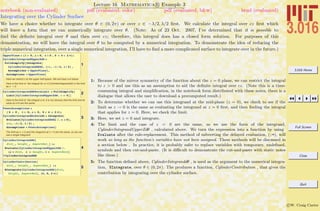
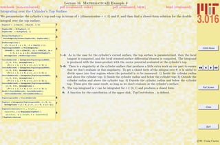
243. 3.016 Home
Full Screen
Close
Quit
c W. Craig Carter
Lecture 16 Mathematica R Example 6
To Evaluate or Not to Evaluate when Defining Functions
notebook (non-evaluated) pdf (evaluated, color) pdf (evaluated, b&w) html (evaluated)
This example illustrates a case in which immediate evaluation = would be preferable to delayed evaluation :=
Let's set a baseline to check efficiency. Here we check timing to integrate
something
1Timing@Integrate@Exp@Tan@xDD, 8x, 0, c<DD
We check the same thing again, because Mathematica may have spent
some time loading algorithms to integrate
2Timing@Integrate@Exp@Tan@xDD, 8x, 0, c<DD
Here, we time how long it takes to create a function (with delayed
assignment), but using Evaluate on the rhs.
3
Timing@DelayedEvaluated@c_D :=
Evaluate@Integrate@Exp@Tan@xDD, 8x, 0, c<DDD
The following is equivalent to the above (safer) definition---and will work
so long as c is not assigned to an expression.
4
Timing@Immediate@c_D =
Integrate@Exp@Tan@xDD, 8x, 0, c<DD
The following should take the *least* amount of time to perform, but as
we shall see is not as efficient in the long run.
5
Timing@FunctionDef@c_D :=
Integrate@Exp@Tan@xDD, 8x, 0, c<DD
6
? DelayedEvaluated
? Immediate
? FunctionDef
The following should give a rapid result
7Timing@DelayedEvaluated@0.5DD
Timing@Immediate@0.5DD
The following will not be rapid, because it has to do the symbolic integra-
tion before returning the result.
8Timing@FunctionDef@0.5DD
1: When a non-trivial integral is done for the first time, Mathematica loads various libraries. Notice
the difference in timing between this first computation of
R
exp[tan(x)]dx and the following one.
2: The second evaluation is faster. Now, a baseline time has been established for evaluating this integral
symbolically.
3: Here, to make a function definition for the integral, the symbolic integral is obtained and so the
function definition takes longer than it would if we had not used Evaluate.
4: Using an = is roughly equivalent to using Evaluate above and the time to make the function
assignment should be approximately the same.
5: Here, the symbolic integration is delayed until the function is called (later). Therefore, the function
assignment is very rapid.
6: We can use the ?-operator to investigate the stored forms of the three function definitions. The first
two forms are roughly equivalent, except for the delayed versus immediate function definition. The
third form uses the unevaluated integral in the definition. symbolic information.
7: The function evaluation is much faster in the case where the symbolic integration is not needed. This
would be the preferred form if the function were to be called many times.
8: The relatively slow speed of the function which contains the unevaluated integral indicates that
it would be a poor choice when numerical efficiency is an issue. Therefore, if we were to use
ContourPlot, or some other function that would need to compute the result at many different points,
then the integration would be done at each point, instead of having its closed form evaluated. Thus,
the function with the embedded closed form is preferable.

244. 3.016 Home
Full Screen
Close
Quit
c W. Craig Carter
Lecture 16 Mathematica R Example 7
Visualizing the Hamaker Potential of a Finite Cylinder: Contours of Constant Potential
notebook (non-evaluated) pdf (evaluated, color) pdf (evaluated, b&w) html (evaluated)
We use the function that we have defined above as the argument to ContourPlot. Because the function is singular at the cylinder surface,
we choose to plot the logarithm of the potential instead. Because the potential is negative outside of the cylinder, we must use an abso-
lute value before taking the log. To remind ourselves that the potential is negative outside the cylinder, we multiply the log by minus-one.
1
LogAbsCyl@r_, h_, AR_D :=
Log@Abs@LondonCylinderPotential@r, h, ARDDD
2
Plot@LogAbsCyl@0.0, h, 4D, 8h, 0, 2.5<,
Exclusions Ø 82.0<, PlotRange Ø 80, 18<,
PlotStyle Ø 8Thick, Darker@BlueD<,
BaseStyle Ø 8Medium<D
3
Plot@LogAbsCyl@x, 0, 1D,
8x, 0.0, 1.5<, Exclusions Ø 81.0<,
PlotRange Ø 80, 20<, PlotStyle Ø 8Thick, Red<,
BaseStyle Ø 8Medium<, ImageSize Ø LargeD
4
conplotouter =
ContourPlot@-LogAbsCyl@dist, h, 4D,
8dist, 0, 1.5<, 8h, 0, 2.5<,
RegionFunction Ø Function@8dist, h<,
dist > 1.01 »» h > 2.01D,
PlotRange Ø 8-15, 1<, Contours Ø 15,
ColorFunction Ø "AvocadoColors",
AspectRatio Ø Automatic,
ImageSize Ø Medium, Exclusions Ø
88dist ã 1.0, Abs@dist - 1.0D < 0.001<,
8h ã 2.0, Abs@h - 2D < 0.001<<D
5
conplotinner =
ContourPlot@LogAbsCyl@dist, h, 4D D,
8dist, 0, 1.5<, 8h, 0, 2.5<, RegionFunction Ø
Function@8dist, h<, dist < 0.99 && h < 1.99D,
PlotRange Ø 80, 15<, Contours Ø 16,
ColorFunction Ø "LakeColors",
AspectRatio Ø Automatic, ImageSize Ø Medium,
BaseStyle -> 8Medium<, AspectRatio Ø Automatic
6Show@conplotinner, conplotouterD
1: We define a short-hand function to wrap around the potential function so that the log(|P|) is com-
puted.
2–3: To get an idea of what the function looks like, we plot the potential first along the cylinder axis,
and then for a distance within the mid-plane.
4: We break the contour-plots into an inner and an outer graphic. Here we use ContourPlot to plot
(minus) the logarithm of the potential outside the cylinder. RegionFunction is used to to limit
the region over which the plot is computed and displayed. Furthermore, the numerical integration is
ill-behaved along lines that continue from the cylinder’s corner; we use Exclusions to avoid these
regions. We use a green tone, AvocadoColors, to indicate the negative values.
5: Here, we produce the contour-plot for the region inside the cylinder. Again, we use the
RegionFunction-option of ContourPlot. We use blue tones, LakeColors, to indicate the posi-
tive potential values.
6: We combine the inner and outer regions into a single plot by using Show.

245. 3.016 Home
Full Screen
Close
Quit
c W. Craig Carter
Lecture 16 Mathematica R Example 8
Visualizing the Hamaker Potential of a Finite Cylinder: Three-Dimensional Plots
notebook (non-evaluated) pdf (evaluated, color) pdf (evaluated, b&w) html (evaluated)
We produce and equivalent visualization with Plot3D. From the form of these plots, it is clear that a non-polar molecule would be
attracted to the cylinder, with a force that becomes unbounded in the vicinity of the cylinder. The barrier to cross into the cylinder is
infinite at the cylinder surface. However, within a cylinder there is a force that pushes a foreign particle to the center of the cylinder.
The Hamaker force would tend to push pores towards the middle of a dielectric cylinder.
1
plotoutside3D =
Plot3D@-LogAbsCyl@dist, h, 4D, 8dist, 0, 1.5<,
8h, 0, 2.5<, RegionFunction Ø Function@
8dist, h<, dist > 1.01 »» h > 2.01D,
PlotRange Ø 8-15, 1<, MeshFunctions -> 8Ò3 &<,
ColorFunction Ø "AvocadoColors",
AspectRatio Ø Automatic,
ImageSize Ø Large, BaseStyle -> 8Medium<,
AspectRatio Ø AutomaticD
2
plotinside3D =
Plot3D@LogAbsCyl@dist, h, 4D, 8dist, 0, 1.5<,
8h, 0, 2.5<, RegionFunction Ø Function@
8dist, h<, dist < 0.99 && h < 1.99D,
PlotRange Ø 80, 15<, MeshFunctions -> 8Ò3 &<,
ColorFunction Ø "LakeColors",
AspectRatio Ø Automatic,
ImageSize Ø Large, BaseStyle -> 8Medium<,
AspectRatio Ø AutomaticD
3Show@plotinside3D,
plotoutside3D, PlotRange Ø 8-15, 15<D
4
1–2: Plot3D is used as in the previous example with the RegionFunction option to separate the inner-
from the outer-evaluation. The MeshFunctions option is used to produce shading that is consistent
with the contour plots in the previous example.
3: We use Show with an extended PlotRange to produce the combined three dimensional surface
representing the potential as a function of distance from the axis cylinder and height above its
mid-plane.

246. 3.016 Home
Full Screen
Close
Quit
c W. Craig Carter
Stokes’ Theorem
The final generalization of the fundamental theorem of calculus is the relation between a vector function integrated over an
oriented surface and another vector function integrated over the closed curve that bounds the surface.
A simplified version of Stokes’s theorem has already been discussed—Green’s theorem in the plane can be written in full
vector form:
R
∂F2
∂x
−
∂F1
∂y
dxdy =
R
× F · dA
=
∂R
(F1dx + F2dy) =
∂R
F ·
dr
ds
ds
(16-6)
as long as the region R lies entirely in the z = constant plane.
In fact, Stokes’s theorem is the same as the full vector form in Eq. 16-6 with R generalized to an oriented surface embedded
in three-dimensional space:
R
× F · dA =
∂R
F ·
dr
ds
ds (16-7)
Plausibility for the theorem can be obtained from Figures 16-14 and 16-15. The curl of the vector field summed over a surface
“spills out” from the surface by an amount equal to the vector field itself integrated over the boundary of the surface. In
other words, if a vector field can be specified everywhere for a fixed surface, then its integral should only depend on some
vector function integrated over the boundary of the surface.
Maxwell’s equations
The divergence theorem and Stokes’s theorem are generalizations of integration that invoke the divergence and curl operations
on vectors. A familiar vector field is the electromagnetic field and Maxwell’s equations depend on these vector derivatives as

247. 3.016 Home
Full Screen
Close
Quit
c W. Craig Carter
well:
· B = 0 × E =
∂B
∂t
× H =
∂D
∂t
+ j · D = ρ
(16-8)
in MKS units and the total electric displacement D is related to the total polarization P and the electric field E through:
D = P + oE (16-9)
where o is the dielectric permittivity of vacuum. The total magnetic induction B is related to the induced magnetic field H
and the material magnetization through
B = µo(H + M) (16-10)
where µo is the magnetic permeability of vacuum.
Ampere’s Law
Ampere’s law that relates the magnetic field lines that surround a static current is a macroscopic version of the (static)
Maxwell equation × H = j:
Gauss’ Law
Gauss’ law relates the electric field lines that exit a closed surface to the total charge contained within the volume bounded
by the surface. Gauss’ law is a macroscopic version of the Maxwell equation · D = ρ:

248. 3.016 Home
Full Screen
Close
Quit
c W. Craig Carter
Oct. 31 2007
Lecture 17: Function Representation by Fourier Series
Reading:
Kreyszig Sections: 11.1, 11.2, 11.3 (pages478–485, 487–489, 490–495)
Periodic Functions
Periodic functions should be familiar to everyone. The keeping of time, the ebb and flow of tides, the patterns and textures of
our buildings, decorations, and vestments invoke repetition and periodicity that seem to be inseparable from the elements of
human cognition.10 Although other species utilize music for purposes that we can only imagine—we seem to derive emotion
and enjoyment from making and experience of music.
10
I hope you enjoy the lyrical quality of the prose. While I wonder again if anyone is reading these notes, my wistfulness is taking a poetic turn:
They repeat themselves
What is here, will be there
It wills, willing, to be again
spring; neap, ebb and flow, wane; wax
sow; reap, warp and woof, motif; melody.
The changed changes. We remain
Perpetually, Immutably, Endlessly.

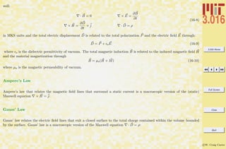
249. 3.016 Home
Full Screen
Close
Quit
c W. Craig Carter
Lecture 17 Mathematica R Example 1
Playing with Audible Periodic Phenomena
notebook (non-evaluated) pdf (evaluated, color) pdf (evaluated, b&w) html (evaluated)
Several example of creating sounds using mathematical functions are illustrated for education and amusement.
Sounds will not be available on PDF or HTML versions
Let's begin by "looking" at a familiar periodic phenomena:
We index the notes and write an indexed set of frequency (in Hertz) for
each of the notes for one octave above middle-c. We write a function to
create a Sound for each note.
1
c = 1; d = 2; e = 3; f = 4; g = 5; a = 6; b = 7;
freq@cD = 261.6;
freq@dD = 293.7;
freq@eD = 329.6;
freq@fD = 349.2;
freq@gD = 392.0;
freq@aD = 440.0;
freq@bD = 493.9;
purenote@note_IntegerD := purenote@noteD =
Play@Sin@2 p freq@noteD tD, 8t, 0, 1<D
We extend the function to get simultaneous notes from a List. We use
Thread which takes f[{a,b,c}] to {f[a],f[b],f[c]}
2
notes@note_ListD :=
Sound@Thread@purenote@noteDDD
Here are examples of their use.
3cnote = purenote@cD
notes@8a, c, e<D
We can play with variable amplitudes for a fixed frequency, here we can
hear the increased, but non-singular amplitude through zero.
4
Plot@Sin@540 xD ê x, 8x, -.1, .1<,
PlotRange Ø All, Filling Ø AxisD
Play@Sin@540 xD ê x, 8x, -1, 1<D
We can vary amplitudes and frequencies. Warning, playing with this
function can become addictive...
5
Play@
2 Sin@20 x Sin@x Exp@-x ê .2D + Sin@xD ê xDD +
Exp@H1 + Cos@xDLD Sin@x Exp@x ê 10DD
Sin@1500 xD, 8x, 0.01, 20<D
1: The seven musical notes around middle C indexed here with integers and then their frequencies (in
hertz) are defined with a freq. The function Note takes one of the seven indexed notes and creates
a wave-form for that note. The function Play takes the waveform and produces audio output. We
introduce a function, purenote , that takes an integer argument and plays the corresponding exact
note.
2: To play a sequence of notes, a list of notes must be passed to Sound. We write a function, notes
, that uses Thread to create a list of object created by applications of purenote. In other words,
Thread[function[{la,lb,lc}]] returns {function[la], function[lb], function[lc]}.
3: This is an example of the use of note and purenote .
4: This is noise generated from a function; we can modulate the amplitude and frequency. Enjoy the
fact that sin(x)/x is not singular at x = 0.
5: This is a function that I cooked up. Enjoy.

250. 3.016 Home
Full Screen
Close
Quit
c W. Craig Carter
Lecture 17 Mathematica R Example 2
Music and Instruments
notebook (non-evaluated) pdf (evaluated, color) pdf (evaluated, b&w) html (evaluated)
Having no musical talent whatsoever, I try to write a program to make music.
Let's see if we can play this:
1twoframes = 8e, e, f, g, g, f, e, d, c, c, d, e<;
We will play it, but it probably not what was intended...
2notes@twoframesD
We create a rest of a fixed length, and then use Riffle to insert a rest
after each note. We use a new function, called SoundNote, with None as
the first argument, we get no sound.
3purenote@restD = SoundNote@None, .15D;
4notes@Riffle@twoframes, restDD
SoundNote can take general strings for arguments as well, here we enter
the musical notes from above (as characters), but one octave lower..
5TwoFramesLower = 8"E3", "E3", "F3", "G3", "G3",
"F3", "E3", "D3", "C3", "C3", "D3", "E3"<;
The default is to use a piano to make the sound; here we ask for a
duration of 6/10 of a second.
6piano@note_StringD := SoundNote@note, .6D
7Sound@Thread@piano@TwoFramesLowerDDD
We can use other MIDI instruments as well; here is a bagpipe
8
bagpipe@note_StringD :=
SoundNote@note, .6, "Bagpipe"D
Sound@Thread@bagpipe@TwoFramesLowerDDD
And, now for the birds.
9
avian@note_StringD :=
SoundNote@note, .2, "Bird"D
avian@restD = SoundNote@None, .4D;
Sound@
Thread@avian@Riffle@TwoFramesLower, restDDDD
1: Someone who knows how to read music told me what these notes were; so, I entered them into a list.
2: This is musical score with one-second duration notes played every 1 second. Oh, Joy.
3: This is probably not what Ludwig Van had in mind; so let’s figure out how to insert a ‘rest.’ We use
Mathematica R ’s built-in SoundNote for .15 seconds to define a purenote for rest rest.
4: Riffle[{l1,l2,l3},x] intersperses x into the list and returns {l1,x,l2,x,l3,x}. Calling notes on
the resulting structure returns the pure notes with rests in between.
5: SoundNote will also play MIDI sounds and take string arguments for notes. We recreate a sting
version of the musical score for notes one octave below middle-c.
6: By default, SoundNote returns a MIDI piano sound. We create a function, piano , to play a single
note for a 0.6 second duration.
7: By using Thread again, we play the 12-note musical score on the piano.
8: There are other MIDI instruments; here we create the function bagpipe and play the score with a
simulated bagpipe.
9: And finally, we introduce a ‘cheep’ little function, avian , to let the birds sing their own joy.

251. 3.016 Home
Full Screen
Close
Quit
c W. Craig Carter
Lecture 17 Mathematica R Example 3
Random Notes and Instruments
notebook (non-evaluated) pdf (evaluated, color) pdf (evaluated, b&w) html (evaluated)
Just because we can, let’s see how sequences of random notes sound. We’ll add random instruments and rests too.
Let's hear what random notes sound like: SoundNote[n] will play n
semitones above middle C. Here we make a list of random notes and
play them.
1
RandomNotes = Table@SoundNote@
RandomInteger@8-15, 20<D, .2D, 836<D;
Sound@RandomNotes, 10D
Here, we mix in some rests at random
2
RanRest@D := Module@8rdur = .2<,
If@RandomReal@D > 0.5, rdur = .4D;
SoundNote@None, rdurDD
RandomNotesandRests =
Table@If@RandomReal@D ¥ .33,
SoundNote@RandomInteger@8-15, 20<D, .2D,
RanRest@DD, 896<D;
Sound@RandomNotesandRests, 20D
Now, we ask for random instruments as well, with "chords" of up to 5
instruments at each beat.
3
RandomInstruments =
Table@If@RandomReal@D > 0.5, Table@
SoundNote@
Table@RandomInteger@8-15, 20<D,
8RandomInteger@81, 5<D<D,
Round@RandomReal@81, 2<D, .2D,
RandomInteger@81, 15<DD,
8RandomInteger@81, 4<D<D, RanRest@DD,
848<D;
Sound@RandomInstruments, 20D
Finally, some random percussion events.
4
percs = 8SoundNote@"Clap", 1D,
SoundNote@"Sticks", 1D, SoundNote@"Shaker",
1D, SoundNote@"LowWoodblock", 1D,
SoundNote@"Castanets", 1D,
SoundNote@None, 1D<;
perctable = Table@RandomChoice@percsD, 850<D;
Sound@perctable, 20D
1: RandomNotes creates a 36 member random set of single pitches from 15 semi-tones below to 20
semi-tones above middle-c. We play them for ten seconds.
2: To introduce some variety into the random melody, we write a program, RanRest , which will be
used to introduce rests with lengths .2 and .4 with equal probability. A list, RandomNotesandRests
, is created with random notes which call RanRest for approximately 1/3 of the members, and from
the same random set as RandomNotes for the remainder.
3: Now, we introduce random MIDI instruments into our score: RandomInstruments is a Table of
length 48, and each member is a list of a random number, between 1 and 5, of random instruments
with random notes. These list-elements create a “chord.” Rests are introduced randomly, at about
1/2 of the beats.
4: Here we play with random percussion MIDI instruments. Dancing to this is not necessarily advised.

252. 3.016 Home
Full Screen
Close
Quit
c W. Craig Carter
A function that is periodic in a single variable can be expressed as:
f(x + λ) = f(x)
f(t + τ) = f(t)
(17-1)
The first form is a suggestion of a spatially periodic function with wavelength λ and the second form suggests a function that
is periodic in time with period τ. Of course, both forms are identical and express that the function has the same value at an
infinite number of points ( x = nλ in space or t = nτ in time where n is an integer.)
Specification of a periodic function, f(x), within one period x ∈ (xo, xo + λ) defines the function everywhere. The most
familiar periodic functions are the trigonometric functions:
sin(x) = sin(x + 2π) and cos(x) = cos(x + 2π) (17-2)
However, any function can be turned into a periodic function.

253. 3.016 Home
Full Screen
Close
Quit
c W. Craig Carter
Lecture 17 Mathematica R Example 4
Using Mod to Create Periodic Functions
notebook (non-evaluated) pdf (evaluated, color) pdf (evaluated, b&w) html (evaluated)
Periodic functions are often associated with the “modulus” operation. Mod[x, λ] is the remainder of the result of recursively dividing x
by λ until the result lies in the domain 0 ≤ Mod[x, λ] < λ). Another way to think of modulus is to find the “point” where are periodic
function should be evaluated if its primary domain is x ∈ (0, λ).
Mod is a very useful function that can be used to force objects to be
periodic. Mod[x,l] return that part of x that lies within 0 and l. Or, in
other words if we map the real line x to a circle with circumference l, then
Mod[x,l] returns were x is mapped onto the circle.
1
modmatdemo@n_Integer, l_IntegerD :=
Table@8i, Mod@i, lD<, 8i, 1, n<D êê
MatrixForm;
modcircledemo@n_Integer, l_IntegerD :=
Module@8xpos, angle, cpos<,
Graphics@
Table@xpos = 3 Quotient@i - 1, lD;
angle = 2 Pi Mod@i, lD ê l;
cpos = 8Cos@angleD, Sin@angleD<;
8Circle@8xpos, 0<D,
Text@i,
Flatten@88xpos, 0< + 1.2 * cpos<DD,
Text@Mod@i, lD, Flatten@88xpos, 0< +
0.8 * cpos<DD<, 8i, 1, n<DDD;
2
GraphicsColumn@
8modmatdemo@13, 5D, modcircledemo@26, 5D<,
ImageSize Ø FullD
Boomerang uses Mod to force a function, f, with a single argument, x, to
be periodic with wavelength l
3Boomerang@f_ , x_ , l_ D := f@Mod@x, lDD
4AFunction@x_ D := HH3 - xL^3L ê 27
The following step uses Boomerang to produce a periodic repetition of
AFunction over the range 0 < x < 6:
5Plot@Boomerang@AFunction, x, 6D,
8x, -12, 12<, PlotRange Ø AllD
1: We create two visualization methods to show how Mod works: modmatdemo creates a matrix with
two columns (i, Mod[i,λ]); modcircledemo wraps the the counting numbers and their moduli
around a Graphics- Circle with a λ sectors, after each circle becomes filled a new circle is created
for subsequent filling. modcircledemo should show how Mod is related to mapping to a periodic
domain.
2: We show both visualization demonstrations in a GraphicsColumn.
3: Boomerang uses Mod on the argument of any function f of a single argument to map the argument
into the domain (0, λ). Therefore, calling Boomerang on any function will create a infinitely periodic
repetition of the function in the domain (0, λ).
4: AFunction is created as an example to pass to Boomerang
5: Plot called on the periodic extension of wavelength λ = 6 of AFunction . This illustrates how
Boomerang uses Mod to create a periodic function with a specified period.

254. 3.016 Home
Full Screen
Close
Quit
c W. Craig Carter
Odd and Even Functions
The trigonometric functions have the additional properties of being an odd function about the point x = 0: fodd : fodd(x) =
−fodd(−x) in the case of the sine, and an even function in the case of the cosine: feven : feven(x) = feven(−x).
This can generalized to say that a function is even or odd about a point λ/2: fodd λ
2
: fodd λ
2
(λ/2 + x) = −fodd λ
2
(λ/2 − x) and
fevenλ
2
: fevenλ
2
(λ/2 + x) = fevenλ
2
(λ/2 − x).
Any function can be decomposed into an odd and even sum:
g(x) = geven + godd (17-3)
The sine and cosine functions can be considered the odd and even parts of the generalized trigonometric function:
eix
= cos(x) + ı sin(x) (17-4)
with period 2π.
Representing a particular function with a sum of other functions
A Taylor expansion approximates the behavior of a suitably defined function, f(x) in the neighborhood of a point, xo, with
a bunch of functions, pi(x), defined by the set of powers:
pi ≡ p = (x0
, x1
, . . . , xj
, . . .) (17-5)
The polynomial that approximates the function is given by:
f(x) = A · p (17-6)
where the vector of coefficients is defined by:
Ai ≡ A = (
1
0!
f(xo),
1
1!
df
dx xo
, . . . ,
1
j!
djf
dxj
xo
, . . .) (17-7)

255. 3.016 Home
Full Screen
Close
Quit
c W. Craig Carter
The idea of a vector of infinite length has not been formally introduced, but the idea that as the number of terms in the sum
in Eq. 17-6 gets larger and larger, the approximation should converge to the function. In the limit of an infinite number of
terms in the sum (or the vectors of infinite length) the series expansion will converge to f(x) if it satisfies some technical
continuity constraints.
However, for periodic functions, the domain over which the approximation is required is only one period of the periodic
function—the rest of the function is taken care of by the definition of periodicity in the function.
Because the function is periodic, it makes sense to use functions that have the same period to approximate it. The simplest
periodic functions are the trigonometric functions. If the period is λ, any other periodic function with periods λ/2, λ/3, λ/N,
will also have period λ. Using these ”sub-periodic” trigonometric functions is the idea behind Fourier Series.
Fourier Series
The functions cos(2πx/λ) and sin(2πx/λ) each have period λ. That is, they each take on the same value at x and x + λ.
There are an infinite number of other simple trigonometric functions that are periodic in λ; they are cos[2πx/(λ/2))] and
sin[2πx/(λ/2))] and which cycle two times within each λ, cos[2πx/(λ/3))] and sin[2πx/(λ/3))] and which cycle three times
within each λ, and, in general, cos[2πx/(λ/n))] and sin[2πx/(λ/n))] and which cycle n times within each λ.
The constant function, a0(x) = const, also satisfies the periodicity requirement.
The superposition of multiples of any number of periodic function must also be a periodic function, therefore any function
f(x) that satisfies:
f(x) = E0 +
∞
n=1
En cos
2πn
λ
x +
∞
n=1
On sin
2πn
λ
x
= Ek0 +
∞
n=1
Ekn cos(knx) +
∞
n=1
Okn sin(knx)
(17-8)
where the ki are the wave-numbers or reciprocal wavelengths defined by kj ≡ 2πj/λ. The k’s represent inverse wavelengths—

256. 3.016 Home
Full Screen
Close
Quit
c W. Craig Carter
large values of k represent short-period or high-frequency terms.
If any periodic function f(x) could be represented by the series in in Eq. 17-8 by a suitable choice of coefficients, then an
alternative representation of the periodic function could be obtained in terms of the simple trigonometric functions and their
amplitudes.
The “inverse question” remains: “How are the amplitudes Ekn (the even trigonometric terms) and Okn (the odd trigonometric
terms) determined for a given f(x)?”
The method follows from what appears to be a “trick.” The following three integrals have simple forms for integers M and
N:
x0+λ
x0
sin
2πM
λ
x sin
2πN
λ
x dx =
λ
2 if M = N
0 if M = N
x0+λ
x0
cos
2πM
λ
x cos
2πN
λ
x dx =
λ
2 if M = N
0 if M = N
x0+λ
x0
cos
2πM
λ
x sin
2πN
λ
x dx = 0 for any integers M, N
(17-9)
The following shows a demonstration of this orthogonality relation for the trigonometric functions.

257. 3.016 Home
Full Screen
Close
Quit
c W. Craig Carter
Lecture 17 Mathematica R Example 5
Orthogonality of Trigonometric Functions
notebook (non-evaluated) pdf (evaluated, color) pdf (evaluated, b&w) html (evaluated)
This is a Demonstration that the relations in Eq. 17-9 are true.
1
fassume = 8Minteger e Integers,
Ninteger œ Integers, xo œ Reals, l > 0<
coscos = Integrate@
Cos@2 p Minteger x ê lD Cos@2 p Ninteger x ê lD ,
8x, xo, xo + l<, Assumptions Ø fassumeD
Demonstrating Ÿxo
xo+l
cosH2 mpx êlL cosH2 npx êlL „ x=0 for m ! n
2
Table@
888mrand, nrand< = RandomInteger@81, 50<, 2D<,
Simplify@coscos ê. 8Minteger Ø mrand ,
Ninteger Ø nrand<D<, 820<D
when n=m give indeterminate values, for these we should use a Limit.
3Limit@coscos, Minteger Ø Ninteger,
Assumptions Ø fassumeD
4
cossin = Integrate@
Cos@2 p Minteger x ê lD Sin@2 p Ninteger x ê lD ,
8x, xo, xo + l<, Assumptions Ø fassumeD
5
Table@
888mrand, nrand< = RandomInteger@81, 50<, 2D<,
Simplify@cossin ê. 8Minteger Ø mrand ,
Ninteger Ø nrand<D<, 820<D
6Limit@cossin, Minteger Ø Ninteger,
Assumptions Ø fassumeD
7
sinsin = Integrate@
Sin@2 p Minteger x ê lD Sin@2 p Ninteger x ê lD ,
8x, xo, xo + l<, Assumptions Ø fassumeD
8
Table@
888mrand, nrand< = RandomInteger@81, 50<, 2D<,
Simplify@sinsin ê. 8Minteger Ø mrand ,
Ninteger Ø nrand<D<, 820<D
9Limit@sinsin, Minteger Ø Ninteger,
Assumptions Ø fassumeD
1: Using Integrate for cos(2πMx/λ) cos(2πNx/λ) over a definite interval of a single wavelength, does
not produce a result that obviously vanishes for M = N.
2: However, random replacement of the symbolic integers with integers results in a zero. So, one the
orthogonality relation is plausible.
3: Using Assuming and Limit, one can show that the relation ship vanishes for N = M. Although, it
is a bit odd to be use continuous limits with integers.
4–6: This shows the same process for
R
cos(2πMx/λ) sin(2πNx/λ)dx, which always returns zeroes.
7–9: And,
R
sin(2πMx/λ) sin(2πNx/λ)dx returns zeroes unless M = N.

258. 3.016 Home
Full Screen
Close
Quit
c W. Craig Carter
Using this orthogonality trick, any amplitude can be determined by multiplying both sides of Eq. 17-8 by its conjugate
trigonometric function and integrating over the domain. (Here we pick the domain to start at zero, x ∈ (0, λ), but any other
starting point would work fine.)
cos(kM x)f(x) = cos(kM x) Ek0 +
∞
n=1
Ekn cos(knx) +
∞
n=1
Okn sin(knx)
λ
0
cos(kM x)f(x)dx =
λ
0
cos(kM x) Ek0 +
∞
n=1
Ekn cos(knx) +
∞
n=1
Okn sin(knx) dx
λ
0
cos(kM x)f(x)dx =
λ
2
EkM
(17-10)
This provides a formula to calculate the even coefficients (amplitudes) and multiplying by a sin function provides a way to
calculate the odd coefficients (amplitudes) for f(x) periodic in the fundamental domain x ∈ (0, λ).
Ek0 =
1
λ
λ
0
f(x)dx
EkN
=
2
λ
λ
0
f(x) cos(kN x)dx kN ≡
2πN
λ
OkN
=
2
λ
λ
0
f(x) sin(kN x)dx kN ≡
2πN
λ
(17-11)
The constant term has an extra factor of two because
λ
0 Ek0 dx = λEk0 instead of the λ/2 found in Eq. 17-9.
Other forms of the Fourier coefficients
Sometimes the primary domain is defined with a different starting point and different symbols, for instance Kreyszig uses
a centered domain by using −L as the starting point and 2L as the period, and in these cases the forms for the Fourier
coefficients look a bit different. One needs to look at the domain in order to determine which form of the formulas to use.

259. 3.016 Home
Full Screen
Close
Quit
c W. Craig Carter
Extra Information and Notes
Potentially interesting but currently unnecessary
The “trick” of multiplying both sides of Eq. 17-8 by a function and integrating comes from
the fact that the trigonometric functions form an orthogonal basis for functions with inner
product defined by
f(x) · g(x) =
λ
0
f(x)g(x)dx
Considering the trigonometric functions as components of a vector:
e0(x) =(1, 0, 0, . . . , )
e1(x) =(0, cos(k1x), 0, . . . , )
e2(x) =(0, 0, sin(k1x), . . . , )
. . . =
...
en(x) =(. . . . . . , sin(knx), . . . , )
then these “basis vectors” satisfy ei · ej = (λ/2)δij, where δij = 0 unless i = j. The trick is
just that, for an arbitrary function represented by the basis vectors, P(x) · ej(x) = (λ/2)Pj.

260. 3.016 Home
Full Screen
Close
Quit
c W. Craig Carter
Lecture 17 Mathematica R Example 6
Calculating Fourier Series Amplitudes
notebook (non-evaluated) pdf (evaluated, color) pdf (evaluated, b&w) html (evaluated)
Functions are developed which compute the even (cosine) amplitudes and odd (sine) amplitudes for an input function of one variable.
These functions are extended to produce the first N terms of a Fourier series.
First we will "do it the hard way" and write short programs that evaluate
Fourier coefficients; then we will demonstrate how to make use of built-in
functions in Mathematica's FourierTransform package…
Define functions based on the formulas derived for the fourier amplitudes
The constant term:
1
EvenTerms@0, function_ , l_D :=
1
l
‡
0
l
function@dumD „dum
A function that defines each even amplitude individually (this is not very
efficient, it would be better to evaluate the integral once and use that
result)
2
EvenTerms@SP_Integer, function_ , l_D :=
EvenTerms@SP, function , wavelengthD =
2
l
‡
0
l
function@dumD CosB
2 SP p dum
l
F „dum
Define the zeroth odd term as zero for symmetry with the even terms:
3OddTerms@0, function_ , l_D := 0
4
OddTerms@SP_Integer, function_ , l_D :=
OddTerms@SP, function , lD =
2
l
‡
0
l
function@dumD SinB
2 SP p dum
l
F „dum
A function to create a vector of amplitudes for the odd terms and one for
the even terms
5
OddAmplitudeVector@
NTerms_Integer, function_, l_D :=
Table@OddTerms@i, function, lD,
8i, 0, NTerms<D
6
EvenAmplitudeVector@
NTerms_Integer, function_, l_D :=
Table@EvenTerms@i, function, lD,
8i, 0, NTerms<D
1–2: EvenTerms computes symbolic representations of the even (cosine) coefficients using the formulas
in Eq. 17-11. The N = 0 term is computed with a supplemental definition because of its extra factor
of 2. The domain is chosen so that it begins at x = 0 and ends at x = λ.
3–4: OddTerms performs a similar computation for the sine-coefficients; the N = 0 amplitude is set to
zero explicitly. It will become convenient to include the zeroth-order coefficient for the odd (sine)
series which vanishes by definition. The functions work by doing an integral for each term—this
is not very efficient. It would be more efficient to calculate the integral symbolically once and then
evaluate it once for each term.
5–6: OddAmplitudeVector and EvenAmplitudeVectors create amplitude vectors for the cosine and sine
terms with specified lengths and domains.
5: This function, f(x) = x(1 − x)2
(2 − x), will be used for particular examples of Fourier series, note
that it is an even function over 0 < x < 2.

261. 3.016 Home
Full Screen
Close
Quit
c W. Craig Carter
Lecture 17 Mathematica R Example 7
Approximations to Functions with Truncated Fourier Series
notebook (non-evaluated) pdf (evaluated, color) pdf (evaluated, b&w) html (evaluated)
Example of using Eq. 17-11 to calculate a Fourier Series for a particular function.
1myfunction@x_ D := Hx * H2 - xL * H1 - xL^2L
2OriginalPlot = Plot@myfunction@xD, 8x, 0, 2<,
PlotStyle Ø 8Hue@.66D, Thickness@0.015D<D
3EvenAmplitudeVector@6, myfunction, 2D
4OddAmplitudeVector@6, myfunction, 2D
5
OddBasisVector@NTerms_Integer, var_, l_D :=
Table@Sin@2 p i var ê lD, 8i, 0, NTerms<D
6OddBasisVector@6, x, 2D
7
EvenBasisVector@NTerms_Integer, var_, l_D :=
Table@Cos@2 p i var ê lD, 8i, 0, NTerms<D
8EvenBasisVector@6, x, 2D
9
FourierTruncSeries@n_, function_, var_ ,
l_D := EvenAmplitudeVector@n, function, lD.
EvenBasisVector@n, var, lD +
OddAmplitudeVector@n, function, lD.
OddBasisVector@n, var, lD
10FourierTruncSeries@6, myfunction, x, 2D
11
FPlot@n_IntegerD := FPlot@nD = Plot@Evaluate@
FourierTruncSeries@n, myfunction, x, 2DD,
8x, -2, 4<, PlotStyle Ø
8Thick, ColorData@n, "ColorList"D<D
12Show@OriginalPlot, FPlot@3D, FPlot@6D,
PlotRange Ø 88-0.5, 2.5<, 8-0.1, 0.26<<D
-0.5 0.5 1.0 1.5 2.0 2.5
-0.10
-0.05
0.05
0.10
0.15
0.20
0.25
1: We introduce and example function x(2 − x)(1 − x2
) that vanishes at x = 0, 1, 2 that will be used to
produce a periodic function with λ = 2item We store the example function’s graphical representation
in OriginalPlot. Note that there will be a sharp discontinuity in the derivative at the edges of the
periodic domain.
3–4: The Fourier coefficients, truncated at six terms, are computed with the functions that we defined
above, OddAmplitudeVector and EvenAmplitudeVector . Note that because of the even symmetry
of the function about the middle, all of the odd coefficients vanish.
5–8: OddBasisVector and EvenBasisVector , create vectors of basis functions of specified lengths and
periodic domains.
9–10: The Fourier series up to a certain order can be defined as the sum of two inner (dot) products:
the inner product of the odd coefficient vector and the sine basis vector, and the inner product of
the even coefficient vector and the cosine basis vector.
11–12: This will illustrate the approximation for a truncated (N = 6) Fourier series. FPlot takes an
integer truncation-argument and generates a plot for that truncation, but only for myfunction. It
might be useful to extend this example so that it takes a function as an argument, but it makes more
sense to leave this example and use Mathematica R ’s built-in Fourier series methods.

262. 3.016 Home
Full Screen
Close
Quit
c W. Craig Carter
Lecture 17 Mathematica R Example 8
Demonstration the used of functions defined in the FourierSeries-package
notebook (non-evaluated) pdf (evaluated, color) pdf (evaluated, b&w) html (evaluated)
Fourier series expansions are a common and useful mathematical tool, and it is not surprising that Mathematica R would have a
package to do this and replace the inefficient functions defined in the previous example.
1Needs@"FourierSeries`"D
2AFunction@x_D :=
Hx - 3L^3
27
3Plot@AFunction@xD, 8x, 0, 6<D
Mathematica's Fourier Series functions are defined for function that are
periodic in the domain x œ (-1/2,1/2). So we need to map the periodic
functions to this domain
4
ReduceHalfHalf@f_ , x_ , l_ D :=
f@Hx + 1 ê 2L * l D
5ReducedFunction =
ReduceHalfHalf@AFunction, x, 6D êê Simplify
8 x3
6
ExactPlot = Plot@ReducedFunction,
8x, -1 ê 2, 1 ê 2<, PlotRange Ø All, PlotStyle Ø
8Red, Opacity@0.5D, Thickness@0.01D<D
7FourierCosCoefficient@ReducedFunction, x, nD
8FourierSinCoefficient@ReducedFunction, x, nD
2 H-1Ln
I6 - n2
p2
M
n3
p3
9FourierTrigSeries@ReducedFunction, x, 5D
2 I-6 + p2M Sin@2 p xD
p3
+
I3 - 2 p2
M Sin@4 p xD
2 p3
+
2 I-2 + 3 p2
M Sin@6 p xD
9 p3
+
I3 - 8 p2M Sin@8 p xD
16 p3
+
2 I-6 + 25 p2M Sin@10 p xD
125 p3
1: The functions in FourierSeries to operate on the unit period located at x ∈ (−1/2, 1/2) by
default. Therefore, the domains of functions of interest can be mapped onto this domain by a change
of variables.
2–3: We introduce another function that will be approximated by a Fourier series. This function will be
made periodic with λ = 6 in the untransformed variables.
4–6: ReduceHalfHalf is an example of a function design to do the required mapping. First the length
of original domain is mapped to unity by dividing through by λ and then the origin is shifted by
mapping the x (that the Mathematica R functions will see) to (−1/2, 1/2) with the transformation
x → x + 1
2
. ReducedFunction shows an example on the function defined above.
8–9: Particular amplitudes of the properly remapped function can be obtained with the functions
FourierCosCoefficient and FourierSinCoefficient. In this example, a symbolic n is entered
and a symbolic representation of the nth
amplitude is returned. Because the function is odd about
the middle, all of the cosine-coefficients are zero.
9: A truncated Fourier series can be obtained symbolically to any order with FourierTrigSeries.

263. 3.016 Home
Full Screen
Close
Quit
c W. Craig Carter
Lecture 17 Mathematica R Example 9
Recursive Calculation of a Truncated Fourier Series
notebook (non-evaluated) pdf (evaluated, color) pdf (evaluated, b&w) html (evaluated)
In this example, we build up a set of recursive function that will be utilized for efficient computation of a truncated Fourier series. These
functions will be used in a subsequent visualization example.
1
ManipulateTruncatedFourierSeries@function_,
8truncationstart_, truncationend_,
truncjump_<D := Manipulate@Plot@Evaluate@
FourierTrigSeries@function, x, itruncDD,
8x, -1, 1<, PlotRange Ø 8-2, 2<D,
8itrunc, 8truncationstart,
truncationend, truncjump<<D;
The function above will work, but it is horribly inefficient! Because it asks
FourierTrigSeries to calculate one more term each time, it is doing some
redundant work. We can fix this up by having
it calculate one new term and adding to the sum calculated previously.
Here it is:
2
costerm@function_, x_, n_IntegerD :=
Simplify@FourierCosCoefficient@
function, x, nDD Cos@2 p n xD
sinterm@function_, x_, n_IntegerD :=
Simplify@FourierSinCoefficient@
function, x, nDD Sin@2 p n xD
TruncatedFourierSeries@function_, x_, 0D :=
TruncatedFourierSeries@function, x, 0D =
costerm@function, x, 0D +
sinterm@function, x, 0D
TruncatedFourierSeries@
function_, x_, n_IntegerD :=
TruncatedFourierSeries@function, x, nD =
TruncatedFourierSeries@function, x, n - 1D +
costerm@function, x, nD +
sinterm@function, x, nD
1: ManipulateTruncatedFourierSeries is a simple example of visualization function for the truncated
Fourier series. It uses the Manipulate function with three arguments in the iterator for the initial
truncation truncationstart, final truncation, and the number to skip in between.
2: However, because the entire series is recomputed for each frame, the function above is not very
efficient. In this second version, only two arguments are supplied to the iterator. At each function
call, the two Nth
Fourier terms are added to those computed in the (N − 1)th
and then stored in
memory. The recursion stops at the defined N = 0 term.

264. 3.016 Home
Full Screen
Close
Quit
c W. Craig Carter
Lecture 17 Mathematica R Example 10
Visualizing Convergence of the Fourier Series: Gibbs Phenomenon
notebook (non-evaluated) pdf (evaluated, color) pdf (evaluated, b&w) html (evaluated)
Functions that produce visualizations with Manipulate (each frame representing a different order of truncation of the Fourier series)
are developed. This example illustrates Gibbs phenomenon where the approximating function oscillates wildly near discontinuities in the
original function. In the Manipulate function, we use the option Initialization so that all evaluations during graphical output will
be rapid.
The following will demonstrate how convergence is difficult where the
function changes rapidly---this is known as Gibbs' Phenomenon
1
Manipulate@GraphicsRow@
8plt = Show@Plot@theapprx@truncationD,
8x, -0.4999, 0.4999<,
PlotRange Ø 88-0.55, 0.55<, 8-1.4, 1.4<<,
PlotStyle Ø 8Thick, ColorData@1,
truncationD<D, ExactPlotD, Show@plt,
PlotRange Ø 880.4, 0.5<, 80.5, 1.2<<D<,
ImageSize Ø FullD,
88truncation, 100<,
1, 100, 1<,
Initialization Ø HTable@
theapprx@iD = TruncatedFourierSeries@
ReducedFunction, x, iD, 8i, 1, 100<D;LD
truncation
1: Because ReducedFunction has a discontinuity (its end-value and its initial-value differ), this vi-
sualization will show Gibbs phenomena near the edges of the domain. The approximation is fine
everywhere except in the neighborhood of the discontinuity. At the discontinuity, the oscillations
about the exact value do not dampen out with increased truncation N, but the domain where the
oscillations are ill-behaved shrinks with increased N.

265. 3.016 Home
Full Screen
Close
Quit
c W. Craig Carter
Complex Form of the Fourier Series
The behavior of the Fourier coefficients for both the odd (sine) and for the even (cosine) terms was illustrated above. Functions
that are even about the center of the fundamental domain (reflection symmetry) will have only even terms—all the sine terms
will vanish. Functions that are odd about the center of the fundamental domain (reflections across the center of the domain
and then across the x-axis.) will have only odd terms—all the cosine terms will vanish.
Functions with no odd or even symmetry will have both types of terms (odd and even) in its expansion. This is a restatement
of the fact that any function can be decomposed into odd and even parts (see Eq. 17-3).
This suggests a short-hand in Eq. 17-4 can be used that combines both odd and even series into one single form. However,
because the odd terms will all be multiplied by the imaginary number ı, the coefficients will generally be complex. Also
because cos(nx) = (exp(inx) + exp(−inx))/2, writing the sum in terms of exponential functions only will require that the
sum must be over both positive and negative integers.
For a periodic domain x ∈ (0, λ), f(x) = f(x + λ), the complex form of the fourier series is given by:
f(x) =
∞
n=−∞
Ckn eıknx
where kn ≡
2πn
λ
Ckn =
1
λ
λ
0
f(x)e−ıknx
dx
(17-12)
Because of the orthogonality of the basis functions exp(ıknx), the domain can be moved to any wavelength, the following is
also true:
f(x) =
∞
n=−∞
Ckn eıknx
where kn ≡
2πn
λ
Ckn =
1
λ
λ/2
−λ/2
f(x)e−ıknx
dx
(17-13)
although the coefficients may have a different form.

266. 3.016 Home
Full Screen
Close
Quit
c W. Craig Carter
Nov. 2 2007
Lecture 18: The Fourier Transform and its Interpretations
Reading:
Kreyszig Sections: 11.4, 11.7, 11.8, 11.9 (pages496–498, 506–512 513–517, 518–523)
Fourier Transforms
Expansion of a function in terms of Fourier Series proved to be an effective way to represent functions that were periodic in an
interval x ∈ (−λ/2, −λ/2). Useful insights into “what makes up a function” are obtained by considering the amplitudes of the
harmonics (i.e., each of the sub-periodic trigonometric or complex oscillatory functions) that compose the Fourier series. That
is, the component harmonics can be quantified by inspecting their amplitudes. For instance, one could quantitatively compare
the same note generated from a Stradivarius to an ordinary violin by comparing the amplitudes of the Fourier components of
the notes component frequencies.
However there are many physical examples of phenomena that involve nearly, but not completely, periodic phenomena—and
of course, quantum mechanics provides many examples of isolated events that are composed of wave-like functions.
It proves to be very useful to extend the Fourier analysis to functions that are not periodic. Not only are the same interpre-
tations of contributions of the elementary functions that compose a more complicated object available, but there are many
others to be obtained.
For example:
momentum/position The wavenumber kn = 2πn/λ turns out to be proportional to the momentum in quantum mechanics.
The position of a function, f(x), can be expanded in terms of a series of wave-like functions with amplitudes that depend

267. 3.016 Home
Full Screen
Close
Quit
c W. Craig Carter
on each component momentum—this is the essence of the Heisenberg uncertainty principle.
diffraction Bragg’s law, which formulates the conditions of constructive and destructive interference of photons diffracting
off of a set of atoms, is much easier to derive using a Fourier representation of the atom positions and photons.
To extend Fourier series to non-periodic functions, the domain of periodicity will extended to infinity, that is the limit of
λ → ∞ will be considered. This extension will be worked out in a heuristic manner in this lecture—the formulas will be
correct, but the rigorous details are left for the math textbooks.
Recall that the complex form of the Fourier series was written as:
f(x) =
∞
n=−∞
Akn eıknx
where kn ≡
2πn
λ
Akn =
1
λ
λ/2
−λ/2
f(x)e−ıknx
dx
(18-1)
where Akn is the complex amplitude associated with the kn = 2πn/λ reciprocal wavelength or wavenumber.
This can be written in a more symmetric form by scaling the amplitudes with λ—let Akn =
√
2πCkn /λ, then
f(x) =
∞
n=−∞
√
2πCkn
λ
eıknx
where kn ≡
2πn
λ
Ckn =
1
√
2π
λ/2
−λ/2
f(x)e−ıknx
dx
(18-2)
Considering the first sum, note that the difference in wave-numbers can be written as:
∆k = kn+1 − kn =
2π
λ
(18-3)
which will become infinitesimal in the limit as λ → ∞. Substituting ∆k/(2π) for 1/λ in the sum, the more “symmetric result”

268. 3.016 Home
Full Screen
Close
Quit
c W. Craig Carter
appears,
f(x) =
1
√
2π
∞
n=−∞
Ckn eıknx
∆k where kn ≡
2πn
λ
Ckn =
1
√
2π
λ/2
−λ/2
f(x)e−ıknx
dx
(18-4)
Now, the limit λ → ∞ can be obtained an the summation becomes an integral over a continuous spectrum of wave-numbers;
the amplitudes become a continuous function of wave-numbers, Ckn → g(k):
f(x) =
1
√
2π
∞
−∞
g(k)eıkx
dk
g(k) =
1
√
2π
∞
−∞
f(x)e−ıkx
dx
(18-5)
The function g(k = 2π/λ) represents the density of the amplitudes of the periodic functions that make up f(x). The function
g(k) is called the Fourier Transform of f(x). The function f(x) is called the Inverse Fourier Transform of g(k), and f(x) and
g(k) are a the Fourier Transform Pair.
Higher Dimensional Fourier Transforms
Of course, many interesting periodic phenomena occur in two dimensions (e.g., two spatial dimensions, or one spatial plus
one temporal), three dimensions (e.g., three spatial dimensions or two spatial plus one temporal), or more.
The Fourier transform that integrates dx√
2π
over all x can be extended straightforwardly to a two dimensional integral of a
function f(r) = f(x, y) by dxdy
2π over all x and y—or to a three-dimensional integral of f(r) dxdydz√
(2π)3
over an infinite three-
dimensional volume.
A wavenumber appears for each new spatial direction and they represent the periodicities in the x-, y-, and z-directions. It

269. 3.016 Home
Full Screen
Close
Quit
c W. Craig Carter
is natural to turn the wave-numbers into a wave-vector
k = (kx, ky, kz) = (
2π
λx
,
2π
λy
,
2π
λy
) (18-6)
where λi is the wavelength of the wave-function in the ith direction.
The three dimensional Fourier transform pair takes the form:
f(x) =
1
(2π)3
∞
−∞
g(k)eık·x
dkxdkydkz
g(k) =
1
(2π)3
∞
−∞
f(x)e−ık·x
dxdydz
(18-7)
Properties of Fourier Transforms
Dirac Delta Functions
Because the inverse transform of a transform returns the original function, this allows a definition of an interesting function
called the Dirac delta function δ(x−xo). Combining the two equations in Eq. 18-5 into a single equation, and then interchanging
the order of integration:
f(x) =
1
2π
∞
−∞
∞
−∞
f(ξ)e−ıkξ
dξ eıkx
dk
f(x) =
∞
−∞
f(ξ)
1
2π
∞
−∞
eık(x−ξ)
dk dξ
(18-8)
Apparently, a function can be defined
δ(x − xo) =
1
2π
∞
−∞
eık(x−ξ)
dk (18-9)

270. 3.016 Home
Full Screen
Close
Quit
c W. Craig Carter
that has the property
f(xo) =
∞
−∞
δ(x − xo)f(x)dx (18-10)
in other words, δ picks out the value at x = xo and returns it outside of the integration.
Parseval’s Theorem
The delta function can be used to derive an important conservation theorem.
If f(x) represents the density of some function (i.e., a wave-function like ψ(x)), the square-magnitude of f integrated over all
of space should be the total amount of material in space.
∞
−∞
f(x) ¯f(x)dx =
∞
−∞
1
√
2π
g(k)e−ıkx
dk
1
√
2π
¯g(κ)e−ıκx
dκ dx (18-11)
where the complex-conjugate is indicated by the over-bar. This exponentials can be collected together and the definition of
the δ-function can be applied and the following simple result can is obtained
∞
−∞
f(x) ¯f(x)dx =
∞
−∞
g(k)¯g(k)dk = (18-12)
which is Parseval’s theorem. It says, that the magnitude of the wave-function, whether it is summed over real space or over
momentum space must be the same.
Convolution Theorem
The convolution of two functions is given by
F(x) = p1(x) p2(x) =
1
√
2π
∞
−∞
p1(η)p2(x − η)dη (18-13)

271. 3.016 Home
Full Screen
Close
Quit
c W. Craig Carter
If p1 and p2 can be interpreted as densities in probability, then this convolution quantity can be interpreted as “the total joint
probability due to two probability distributions whose arguments add up to x.”11
The proof is straightforward that the convolution of two functions, p1(x) and p2(x), is a Fourier integral over the product of
their Fourier transforms, ψ1(k) and ψ2(k):
p1(x) p2(x) =
1
√
2π
∞
−∞
p1(η)p2(x − η)dη =
1
√
2π
∞
−∞
ψ1(k)ψ2(k)eıkx
dk (18-14)
This implies that Fourier transform of a convolution is a direct product of the Fourier transforms ψ1(k)ψ2(k).
Another way to think of this is that “the net effect on the spatial function due two interfering waves is contained by product
the fourier transforms.” Practically, if the effect of an aperture (i.e., a sample of only a finite part of real space) on a wave-
function is desired, then it can be obtained by multiplying the Fourier transform of the aperture and the Fourier transform
of the entire wave-function.
11
To think this through with a simple example, consider the probability that two dice sum up 10. It is the sum of p1(n)p2(10−n) over all possible
values of n.

272. 3.016 Home
Full Screen
Close
Quit
c W. Craig Carter
Lecture 18 Mathematica R Example 1
Creating Images of Lattices for Subsequent Fourier Transform
notebook (non-evaluated) pdf (evaluated, color) pdf (evaluated, b&w) html (evaluated)
A matrix of intensities (or, the density of scattering objects) is created as a set of “pixels” for imaging. We will use data like this to simulate
Here we create an image simulating what
might be seen in an electron microscope. We
will use this data to perform simulated diffrac-
tion through use of Fourier Transforms.
1
ISize = 64;
AtomDensity =
N@Table@H1 + Sin@4 Hx + yL
2 Pi ê ISizeDL
H1 + Sin@2 Hx - 2 yL 2
Pi ê ISizeDL ê 4,
8x, 1, ISize<, 8y,
1, ISize<DD;
2
GraphicsRow@
8ArrayPlot@AtomDensityD,
ListPlot3D@AtomDensityD<,
ImageSize Ø FullD
1: Table to form a discrete set of points that we will use to approximate am image which image such as
might be seen in an transmission electron microscope. For our first set of data, we use interference of
two sine waves to produce a simulation of the density of scattering centers in an atomic lattice. Most
of the physical aspects of atomic imaging and diffraction can be simulated with the two-dimensional
techniques that are produced in these notes. We start with a 64 × 64 set of discrete points, this is
fairly small but it will produce fairly computationally inexpensive results.
2: ArrayPlot produces a gray-scale image from an array of “pixel values” between 0 (black) and 1
(white); we use Plot3D to get an additional visualization of the density of scatterers.

273. 3.016 Home
Full Screen
Close
Quit
c W. Craig Carter
Lecture 18 Mathematica R Example 2
Improving Visualization Contrast with ColorFunction
notebook (non-evaluated) pdf (evaluated, color) pdf (evaluated, b&w) html (evaluated)
Two examples of ColorFunction, normalcontrast and highcontrast are produced that aid in the interpretation of simulated data. The
first, normalcontrast , provides a way to use a color, red, to interpolate between black at low intensities and white at high intensities.
The second, highcontrast , compresses the color change at the low-intensity end; this provides a means to visualize “noise” at low intensities.
A
To view the data better, we create
two versions of a contrast function,
the first (normalcontrast) is useful
when we wish to view the entire
range of intensities, the second
version (highcontrast) when we wish
to resolve differences at the low-end
of the intensities.
4ContrastGraphics
normalcontrast
highcontrast A: Three input expressions are not shown, but available in the links provided above. The first two
define the two Pure Functions that will be used at the ColorFunction option to graphics objects.
The third produces a scale that relates the colors to the intensities.
4: ContrastGraphics , defined in item A, shows the relation of colors to intensity.

274. 3.016 Home
Full Screen
Close
Quit
c W. Craig Carter
Lecture 18 Mathematica R Example 3
ImagePlot
notebook (non-evaluated) pdf (evaluated, color) pdf (evaluated, b&w) html (evaluated)
This will be our swiss-army knife visualizer for atomic image and diffraction image graphics.
1
ImagePlot@data_?MatrixQ,
label_: None,
colfunc_: highcontrast,
imagesize_: MediumD :=
Module@8absdata =
Abs@dataD, min, max<,
ArrayPlot@absdata,
ColorFunction Ø colfunc,
BaseStyle Ø
8Tiny, FontFamily Ø
"Helvetica"<,
PlotLabel Ø label,
ImageSize Ø imagesizeDD
1: ImagePlot takes a rectangular array of (possibly complex-valued) intensities are produces graphics
from them. It takes three optional functions for the PlotLabel, ColorFunction, and ImageSize
which will have default values if not given. It uses Abs to find the magnitude of each pixel and
then ArrayPlot to visualize it. Note, the units of the graphics are the number of pixels along the
horizontal and vertical edges.

275. 3.016 Home
Full Screen
Close
Quit
c W. Craig Carter
Discrete Fourier Transforms
The fast fourier transform (FFT) is a very fast algorithm for compute discrete Fourier transforms (DFT) (i.e., the Fourier
transform of a data set) and is widely used in the physical sciences. For image data, the Fourier transform is the diffraction
pattern (i.e., the intensity of reflected waves from a set of objects, the pattern results from positive or negative reinforcement
or coherence).
However, for FFT simulations of the diffraction pattern from an image, the question arises on what to do with the rest of space
which is not the original image. In other words, the Fourier transform is taken over all space, but the image is finite. In the
examples that follow, the rest of space is occupied by periodic duplications of the original image. Thus, because the original
image is rectangular, there will always be an additional rectangular symmetry in the diffraction pattern due to scattering
from the duplicate features in the neighboring images.
The result of a discrete Fourier transform is a also a discrete set. There are a finite number of pixels in the data, the same
finite number of sub-periodic wave-numbers. In other words, the Discrete Fourier Transform of a N × M image will be a data
set of N × M wave-numbers:
Discrete FT Data = 2π(
1
Npixels
,
2
Npixels
, . . . ,
N
Npixels
)
×2π(
1
Mpixels
,
2
Mpixels
, . . . ,
M
Mpixels
)
(18-15)
representing the amplitudes of the indicated periodicities.

276. 3.016 Home
Full Screen
Close
Quit
c W. Craig Carter
Lecture 18 Mathematica R Example 4
Discrete Fourier Transforms on Simulated Lattices
notebook (non-evaluated) pdf (evaluated, color) pdf (evaluated, b&w) html (evaluated)
Example of taking the Discrete Fourier Transform (DFT) of the simulated lattice created above and visualizing it Fourier transform.
We create a function that shows the original
data, its Fourier transform, and then its
inverse transform (hopefully) back to the
original image.
1
FourierRow@data_D :=
Module@8fourdat =
Fourier@dataD<,
GraphicsRow@
8ImagePlot@data, "",
normalcontrastD,
ImagePlot@fourdatD !,
ImagePlot@
InverseFourier@
fourdatD, "",
normalcontrastD<,
ImageSize Ø SmallDD
Peaks will be located located near (kx,ky) =
2 p (a,b)/(size), where (a,b) = {(0,0), (size,0),
(0,size), (size, size)}. These correspond to
the longest wavelength periodicities.
2FourierRow@AtomDensityD
Original
Data
Fourier
Transform H! L
! -1
@! @OriginalDD,
1: FourierRow is a function to visualize, from left to right, the input intensity data, its Fourier trans-
form, and the inverse Fourier Transform of the Fourier Transform. If the final image isn’t the same
as the first, then something went dreadfully wrong.
2: Notice that the Fourier Transform has very sharp features at the corners of the figure; this is because
the original data lattice is a linear combination of sine waves. There are three unique peaks in the
pattern. The first, and brightest, sits at (kx, ky) = (2π/λx, 2π/λy) = (1, Ny). This peak comes from
each pixel interfering with itself in a periodic repetition of the underlying rectangular (in this case,
square) lattice. As the number of pixels becomes large, this peak converges to the infinite wavelength
limit (or the data with no periodic correlations). This brightest peak is, in fact, the super position
of four periodic peaks; the other three are at: (1 + Nx, 1), (1 + Nx, 1 + Ny), and (Nx, 1 + Ny). The
reason it appears in the upper left is related to our approximation of dx and dy with 1/Nx and 1/Ny
and the underlying periodicity of the image: there are four choices on which corner to use as the
bright spot, upper-left is the one that appears.
The second brightest peak is located at ◦
45 to the highest intensity peak. The peak derives from the
sin(x + y) in one of superposed waves—it is the signature of the planes oriented at ◦
45 (11) in the
original data. Each peak corresponds to the superposition of two waves, and its intensity is one-half
of the brightest spot which is the superposition of four.
There are just as many low-intensity peaks as mid-intensity. These peaks are derive from the x − 2y
modulated sine-wave; their intensity is less because the distance between the corresponding planes
is larger.

277. 3.016 Home
Full Screen
Close
Quit
c W. Craig Carter
Lecture 18 Mathematica R Example 5
Simulating Diffraction Patterns
notebook (non-evaluated) pdf (evaluated, color) pdf (evaluated, b&w) html (evaluated)
Materials scientists, microscopists, and crystallographers observe the long wavelength peak at the middle of the diffraction pattern. We
develop a data manipulation function that takes input data and outputs the same data, but with our approximation to k = 0 at the center.
Materials Scientists, Microscopists, and
Crystallographers are used to seeing the k =0
spot at the center of the diffraction image; so
we write a function that takes the Fourier data
and manipulates to so as to move spots to the
center.
1
KZeroMiddle@
fourmat_?MatrixQD :=
Module@8nrows, ncols<,
8nrows, ncols< =
Dimensions@fourmatD;
RotateRight@fourmat,
8Quotient@nrows, 2D,
Quotient@ncols, 2D<DD
A
And, we modify our FourierRow
function to use the k-at-zero
transformation: FourierRowK0
3FourierRowK0@AtomDensityD
Original
Data
! @dataD
k =0 centered
! -1
@! @OriginalDD
1: KZeroMiddle uses RotateRight to “rolls” the data array so that the left edge goes to the center,
followed by the right edge which ends up just to its left at the center; the two columns at the center
roll to both edges. The same operation is performed in the vertical direction. To find the center, we
use Quotient instead of dividing the number of columns and rows by 2 to anticipate the cases where
there is an odd number of rows or columns. Fourier transform of the diffraction image are viewed
side-by-side.
A–3: FourierRowK0 duplicates the functionality of FourierRow , but the Fourier data is filtered with
KZeroMiddle before display. The definition of the graphics function is straightforward and sup-
pressed in these class notes versions. This simulates an observed fraction pattern, but with colors
instead of gray-scale to indicate intensity of the image’s periodicities. KZeroAtCenter divides the
original matrix data into four approximately equal-sized parts,

278. 3.016 Home
Full Screen
Close
Quit
c W. Craig Carter
Lecture 18 Mathematica R Example 6
Alternative Representations of Diffraction Data
notebook (non-evaluated) pdf (evaluated, color) pdf (evaluated, b&w) html (evaluated)
Because our data is organized as intensities over the x–y plane we can use the z-direction to add another component to visualization.
We can also use the same contrast function that we employed for the two-dimensional simulation.
1
Spots3D@data_,
range_: AllD :=
ListPlot3D@KZeroMiddle@
Abs@Fourier@dataDDD,
ColorFunction Ø
Hhighcontrast@Ò3D &L,
PlotRange Ø rangeD
2
Spots3DRow@data_,
range_D := Module@8plt<,
plt = Spots3D@dataD;
GraphicsRow@
8plt, Show@plt,
PlotRange Ø rangeD<DD
3Spots3DRow@
AtomDensity, 80, 7<D
1: Spots3D uses ListPlot3D to convert our discrete two-dimensional data into a Graphics3D object.
We create a default argument for the range of intensities to be plotted, and use highcontrast on the
z-values.
2–3: Spots3DRow takes Fourier data and creates visualizations for the all the intensities, and a second
argument for a range, which permits us to observe the finer structure of the diffraction intensities. In
this case, because the data is the superposition of two sine-waves, discrete approximations to sharp
peaks are observed.

279. 3.016 Home
Full Screen
Close
Quit
c W. Craig Carter
Lecture 18 Mathematica R Example 7
Diffraction Patterns of Defective Lattices
notebook (non-evaluated) pdf (evaluated, color) pdf (evaluated, b&w) html (evaluated)
In this example, the simulated atomic density is modified to simulate the removal of one atom—in other words, we simulate a vacancy.
A
Algorithm to Create a Defect in a
Simulated Atomic Density Image :
Here, the algorithm will create new
data which will be called
AtomDensityWithDefect
2FourierRowK0@
AtomDensityWithDefectD
Original
Data
! @dataD
k =0 centered
! -1
@! @OriginalDD
3
Spots3DRow@
AtomDensityWithDefect,
80, 1 ê 2<D
A: AtomDensityWithDefect are simulated data with a vacancy (definition-algorithm suppressed in class
notes). It selects one of the maximum intensity positions at random, and then sets data in, disk
centered at that position, to zero.
2–3: The vacancy affects the diffraction pattern with diffuse, low-intensity scattering near k = 0. The
3D version shows more clearly that the peaks remain the dominate feature, and we have to decrease
the range to very small intensities to find the defect scattering all. Nevertheless, the intensity that
is shed from the peaks into the entire spectrum reproduces the defect on the reconstructed image.

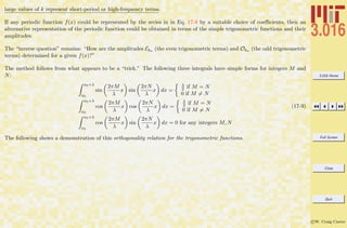
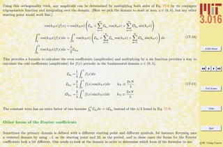
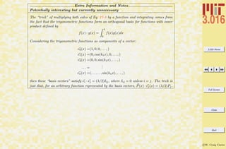
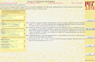
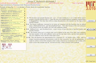
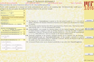
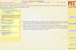
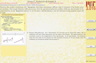
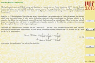
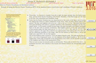
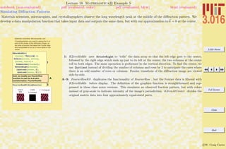
280. 3.016 Home
Full Screen
Close
Quit
c W. Craig Carter
Lecture 18 Mathematica R Example 8
Diffraction Patterns from Lattices with Thermal ‘Noise’
notebook (non-evaluated) pdf (evaluated, color) pdf (evaluated, b&w) html (evaluated)
Functions to create a two-dimensional lattices of squares with a specifiable amount of randomness in their position are created. are
developed with a variable that simulates random deviation from their ideal lattice positions.
A
Function to Create A Lattice of
Squares :
NoisyLattice[TotalSize,
LatticeVector1, LatticeVector2,
SquareSize,
RandomDisplacements]
2
NoNoise =
NoisyLattice@64, 88, 4<,
816, 16<, 1, 80, 0<D;
3
FourierRowK0@NoNoiseD
GraphicsRow@
8Spots3D@NoNoiseD,
Spots3D@NoNoise, 80, 2<D<D
4
SomeNoise =
NoisyLattice@64, 88, 4<,
816, 16<, 1, 81, 1<D;
FourierRowK0@SomeNoiseD
GraphicsRow@
8Spots3D@SomeNoiseD,
Spots3D@SomeNoise,
80, 2<D<D
A: NoisyLattice ’s first argument is the size N of the N × N that is returned. It also takes input for the
two lattice-vectors, the size of squares to place near the lattice positions, and a vector that specifies
the magnitude of random displacements in the x and y directions. (The definition, which is a bit
long and complicated, is suppressed in the class-notes.) This function will produce smaller unit cells
if the lattice vectors are divisors of the data size.
2–3: This simulates data from ‘perfect’ lattice of squares. Note, that in this case, the entire diffrac-
tion pattern is filled. This is because the original data are not sine-waves, but superposed square-
wave-patterns. This diffraction pattern is called the reciprocal lattice by materials scientists and
crystallographers.
4: The data from SomeNoise will illustrate the effect of adding isotropic thermal noise (in a real crystal,
the amplitude of the noise will be larger in the elastically soft directions, it would not be difficult
to modify this function to take a matrix of compliances to multiply the random displacements) A
diffuse ring of scattering about k = 0 is superimposed onto the ‘ideal’ diffraction pattern.

281. 3.016 Home
Full Screen
Close
Quit
c W. Craig Carter
Lecture 18 Mathematica R Example 9
Computational Microscopy
notebook (non-evaluated) pdf (evaluated, color) pdf (evaluated, b&w) html (evaluated)
We produce functions to create circular apertures and interactively move and resize the apertures on the diffraction pattern.
Transmission electron microscopy works by accelerating electrons with a voltage difference and sending them towards a target. The
electrons interact with the target and scatter. After the electrons have passed through the sample, they are focused with a magnetic
objective lens (or typically lenses). This lens produces a plane at which electrons scattered in the same direction arrive at the same
point—this is the diffraction pattern. Because diffraction transforms periodic elements into points, it is closely related to the fourier
transform. An image of the target is created beyond this diffraction plane. An operator of an electron microscope can toggle between
looking at the diffraction-plane or the image-plane.
The “Bright-Field Image” consists of using a central aperture around the direct beam to block off all others from contributing to the
image.
The “Dark-Field Image” consists of selecting a specific diffracted peak with the aperture and using that to form an image.
A “Structure image,” or a “lattice image,” uses the direct beam and one or more diffracted beams to form the image. In this case, the
apertures are typically much larger than for bright- or dark-field imaging.
Aperture size is effectively limited because of spherical aberrations that become significant for beams that are “off-axis” by a significant
amount. So, in practice one can only use part of the Fourier spectrum (reciprocal space) to produce an image in TEM. You always lose
some structure information in the image formation.
A
Function to Create Two Circular
Aperatures (i.e, to remove all data
from a Fourier Transform except the
regions inside two specified circles:
CircAps[Center1, Center2, Radius1,
Radius2, FourierData]
B
Function to Perform Diffraction Spot
Microscopy on Real-Space Images
DiffractionMicroscopy[RealData]
Creates a Interactive Structure with
Four Windows Arranged in a Square.
NorthWest: All Fourier Data from
Real Image with Movable
Aperatures, use a clicked mouse to
move aperatures to various
diffraction peaks.
NorthEast: The original real
space image.
SouthWest: The Fourier image of
the aperature filtered data. (Don't try
to move these aperatures)
SouthEast: The reconstructed
image from the aperature filtered
data.
A: CircAps is a function (definition suppressed in class-notes) designed to take the positions of the
centers of two circular apertures, their radii, and input data (which is intended to be the Fourier
transform of scattering density. It returns the data with zeroes everywhere except within the aper-
tures, where it has the same value as the input data.
B: DiffractionMicroscopy (definition suppressed, but available at the links given above) takes an array
of values representing scattering density, and creates an interactive simulation which allows the user
to move the apertures with the mouse, and their radii with slider controls. This definition is only
about 20 lines of code, and demonstrates the economy of Mathematica R 6’s new Manipulate
function. We will demonstrate examples below.

282. 3.016 Home
Full Screen
Close
Quit
c W. Craig Carter
Lecture 18 Mathematica R Example 10
Visualizing Simulated Selected Area Diffraction
notebook (non-evaluated) pdf (evaluated, color) pdf (evaluated, b&w) html (evaluated)
We create a function that creates a square array of square “grains”. Each grain will be simplified by creating a sinusoidal modulation
in each of the Ng × Ng with a random orientation picked from an equally spaced set of angles in (0, N2
g π).
A
GrainStructure[TotalSize,
GrainSize]
Creates an array of "square
grains" with stripes oriented in
somewhat random orientations
2
Grains =
GrainStructure@128, 64D;
ImagePlot@Grains,
"Simulated
Grain Structure",
normalcontrast, LargeD
Simulated Grain Structure A: This is a definition of the function GrainStructure (suppressed in class-notes). Its first argument is
the number of pixels along one side of the image, and the second is the number of pixels along the
side of the grains. It is best to make the grain size a divisor of the image size.
2: This is an example of creating data and imaging it for a 2 × 2 grain structure.

283. 3.016 Home
Full Screen
Close
Quit
c W. Craig Carter
Lecture 18 Mathematica R Example 11
Simulated Diffraction Imaging on a Polycrystal
notebook (non-evaluated) pdf (evaluated, color) pdf (evaluated, b&w) html (evaluated)
We use our simulated grain structure as input to our diffraction simulator, DiffractionMicroscopy .
Diffraction Spot Microscopy on grain structure.
1DiffractionMicroscopy@
GrainsD
Purple
Radius
Fourier Representation of Data
Click on Aperatures to Move
Input
Data
Selected Fourier DataFiltered Image
Yellow
Radius
1: Here is an example of our interactive function, DiffractionMicroscopy , on a polycrystal. You can
move each aperture by mouse-dragging and control their sizes with the sliders. You can only move
the apertures in the upper-left image. Try these simple experiments first:
Image Orientation of a Single Grain: Move the purple aperture over on of the green diffraction peaks.
Notice that only one grain is imaged in the reconstruction. Because the yellow aperture is picking
up data from the k = 0 spot, the other aperture is producing the modulation of a single sine wave.
Imaging a Single Grain: Shrink the yellow aperture to zero; this is a “dark-field” simulation. Move
the purple aperture over a single peak; notice that a single grain is imaged, but its modulation has
disappeared.
Imaging a Defect: Keeping the yellow aperture at zero-radius, move the purple apertures over one
of the streaks in the diffraction pattern. Notice that a grain boundary is imaged—pay attention to
the orientation of the grain boundary relative to that of the streak in the diffraction image.

284. 3.016 Home
Full Screen
Close
Quit
c W. Craig Carter
Lecture 18 Mathematica R Example 12
Bright-Field and Dark-Field Imaging of a Lattice with Thermal Noise
notebook (non-evaluated) pdf (evaluated, color) pdf (evaluated, b&w) html (evaluated)
We use our ideal lattice of squares and a similar one with a bit of thermal noise to continue our investigation of diffraction phenomena.
1DiffractionMicroscopy@
NoNoiseD
2DiffractionMicroscopy@
SomeNoiseD
Purple
Radius
Fourier Representation of Data
Click on Aperatures to Move
Input
Data
Selected Fourier DataFiltered Image
Yellow
Radius
1: Here, we use our computational microscope, DiffractionMicroscopy , on an ideal lattice. Here are
some experiments to try:
Image a Set of Planes Leave the yellow aperture over the k = 0 peak. Move the purple aperture one
of the nearby spots. Notice the orientation and periodicity of the planes in the reconstructed image.
Detect Periodicity Leave the yellow aperture at k = 0. Move the purple aperture from one of
the nearby peaks to a similarly oriented one along the same ray from the origin. Notice that the
orientation of the planes do not change, but the period of modulation is increased. (Also, recall
that this is a complex superposition of sine-waves to make squares, in the simple superposition of
sine-waves, there we fewer peaks.)
2: Here, we do the same example with our randomly perturbed lattice of squares. There is a significant
amount of diffuse scattering, but by observing carefully, you will see the the same peaks that were
present for the perfect lattice.
Discover Robustness of Imaging with Noise If you leave the yellow aperture over k = 0, and move
the purple aperture over one of the “perfect peaks,” you will see a reconstruction of perfect planes
even though they are barely discernible in the original image. If you shrink the purple radius, while
leaving it over the peak, you will see the quality of the planes improves as less diffuse scattering is
included. This simulates how a microscopist can image individual atom planes at finite temperatures
where atoms are vibrating around their equilibrium positions.

285. 3.016 Home
Full Screen
Close
Quit
c W. Craig Carter
Lecture 18 Mathematica R Example 13
Selected Area Diffraction on Image Data
notebook (non-evaluated) pdf (evaluated, color) pdf (evaluated, b&w) html (evaluated)
DiffractionMicroscopy is used on data that is extracted from a gray-scale image-file.
1
AnImage = Import@
"http:êêpruffle.mit.eduê
3.016-2007êMsChang.
pgm"D
2DiffractionMicroscopy@
1 - ChangDataD
1: We read in an image that is stored on the ‘net. We do a bit of plastic surgery on this data to put it
into a form that is ready for our microscope (plastic surgery algorithm suppressed in class-notes)
2: We perform selected area diffraction on this image. Notice that we can highlight different aspects of
the image by selecting different aperture locations.

286. 3.016 Home
Full Screen
Close
Quit
c W. Craig Carter
Nov. 5 2007
Lecture 19: Ordinary Differential Equations: Introduction
Reading:
Kreyszig Sections: 1.1, 1.2, 1.3 (pages2–8, 9–11, 12–17)
Differential Equations: Introduction
Ordinary differential equations are relations between a function of a single variable, its derivatives, and the variable:
F
dny(x)
dxn
,
dn−1f(x)
dxn−1
, . . . ,
d2y(x)
dx2
,
dy(x)
dx
, y(x), x = 0 (19-1)
A first-order Ordinary Differential Equation (ODE) has only first derivatives of a function.
F(
dy(x)
dx
, y(x), x) = 0 (19-2)
A second-order ODE has second and possibly first derivatives.
F
d2y(x)
dx2
,
dy(x)
dx
, y(x), x = 0 (19-3)
For example, the one-dimensional time-independent Shr¨odinger equation,
−
2m
d2ψ(x)
dx2
+ U(x)ψ(x) = Eψ(x)
or
−
2m
d2ψ(x)
dx2
+ U(x)ψ(x) − Eψ(x) = 0

287. 3.016 Home
Full Screen
Close
Quit
c W. Craig Carter
is a second-order ordinary differential equation that specifies a relation between the wave function, ψ(x), its derivatives, and
a spatially dependent function U(x).
Differential equations result from physical models of anything that varies—whether in space, in time, in value, in cost, in
color, etc. For example, differential equations exist for modeling quantities such as: volume, pressure, temperature, density,
composition, charge density, magnetization, fracture strength, dislocation density, chemical potential, ionic concentration,
refractive index, entropy, stress, etc. That is, almost all models for physical quantities are formulated with a differential
equation.
The following example illustrates how some first-order equations arise:
Iterative Application of Function

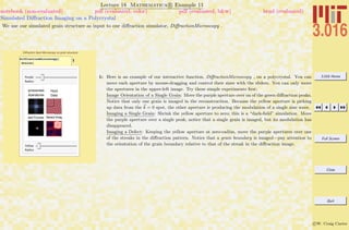
288. 3.016 Home
Full Screen
Close
Quit
c W. Craig Carter
Lecture 19 Mathematica R Example 1
Iteration: First-Order Sequences from a Fixed Boundary Condition
notebook (non-evaluated) pdf (evaluated, color) pdf (evaluated, b&w) html (evaluated)
Sequences are developed in which the next iteration only depends on the current value; in this most simple case simulate exponential
growth and decay.
Suppose a function, F[i], changes propor-
tional to its current size, i.e., F[i+1] = F[i] +
aF[i]
1
ExplFun@i_, a_D :=
ExplFun@i, aD =
ExplFun@i - 1, aD +
a * ExplFun@i - 1, aD
In the above, the symbol is assigned (Expl-
Fun[i,alpha] = ...) as part of the function
definition, so that intermediate values are
``remembered.''
The function needs some value at some time
(an initial condition) from which it obtains all its
other values:
2ExplFun@0, 0.25D = p ê 4
3ExplFun@18, 0.25D
1: ExpleFun taking two arguments is defined: the first argument represents the iteration and the second
represents a single parameter expressing how the current iteration grows. The value at the i + 1th
iteration is the sum of the value of the ith
plus α times value of the ith
iteration. If this is a bank
account and interest is compounded yearly, then the ith
iteration is the value of an account after
i years at a compounded annual interest rate of α. This function has improved performance (but
consumes more memory) by storing its intermediate values.
2: Of course, the function would iterate for ever if an initial value is not specified; and so it is specified
here.
3: For, example this would produce the 18th
iteration of growth with a compounding rate of 25% with
π/4 at the initial state.

289. 3.016 Home
Full Screen
Close
Quit
c W. Craig Carter
Lecture 19 Mathematica R Example 2
Iteration: First-Order Sequences with a Generalized Boundary Condition
notebook (non-evaluated) pdf (evaluated, color) pdf (evaluated, b&w) html (evaluated)
The previous example is generalized so that the iteration function is generalized for an arbitrary initial values.
1
ExplFun@0 , a_,
InitVal_D := InitVal
ExplFun@Inc_Integer,
a_, InitVal_D :=
ExplFun@Inc, a, InitValD =
ExplFun@Inc - 1, a,
InitValD + a * ExplFun@
Inc - 1, a, InitValD
2
Traj@
Steps_Integer ?Positive,
a_, InitVal_D :=
Traj@Steps, a, InitValD =
AppendTo@Traj@Steps - 1,
a, InitValD, ExplFun@
Steps, a, InitValDD
Traj@0, _, _D = 8<;
3Traj@12, .01, .001D
A
We define a function, Evolve,
producing an interactive tool with
input : Initial values and a.producing
an interactive tool with input : Initial
values and a.
5Evolve@300D
1: Because the initial value and the ‘growth factor’ α determine all subsequent iterations, it is sensible
to ‘overload’ ExplFun (i.e., define the function to behave differently depending on the number and
type of its arguments) to take an extra argument for the initial value. Here, if ExplFun is called
with three arguments and the first argument is zero, then the initial value is set; otherwise it is a
recursive definition with intermediate value storage.
2: Traj is an example of a function that builds a list by first-order iteration. It produces a result that
is suitable for input to ListPlot. The second part of the definition defines the 0th
item of the list
to always be an empty list, no matter what other values are passed to it. Traj does its work by
calculating new pairs with the help of ExplFun and then recursively appends the current value to
the growing list.
3: Here is an example which will produce a list of twelve entries, starting from the first iteration of
0.001 with growth factor of 1%.
8: To visualize the behavior as a function of its initial value, an interactive function, Evolve , is defined
(definition suppressed in notes, but available via the links). It takes an argument for the maximum
number of iterations, and the initial value and growth factor are controlled with Manipulate.

290. 3.016 Home
Full Screen
Close
Quit
c W. Craig Carter
Lecture 19 Mathematica R Example 3
Space-Covering Sequences: Families of Trajectories
notebook (non-evaluated) pdf (evaluated, color) pdf (evaluated, b&w) html (evaluated)
The previous example is generalized so that the iteration function is generalized for an arbitrary initial values. several plots. Once the
growth rate is fixed, we visualize how each curve “belongs” to a particular initial value; the set of all initial values generates a family of
curves that fill the plane—each point belongs to one and only one trajectory.
Plotting a bunch of curves for the same
positive a value, but each corresponding to a
different initial value.
1
PlotTrajs@a_D := Block@
8$RecursionLimit = 10^4<,
ListPlot@Evaluate@
Table@Traj@300, a, ivD,
8iv, -1, 1, 0.25<DD,
PlotRange Ø All,
Joined Ø True,
PlotStyle Ø ThickDD
2PlotTrajs@0.02D
20 40 60 80 100
-6
-4
-2
2
4
6
3PlotTrajs@-0.02D
20 40 60 80 100
-1.0
-0.5
0.5
1.0
1: PlotTrajs is a function that provides a visualization of trajectories for an input growth. It works by
generating a set of initial values to pass to Traj and then plots them with ListPlot.
2: If α > 0, the function goes to ±∞ depending on the sign of the initial value. For a fixed α every
point in the plane belongs to one and only one trajectory associated with an initial value and that
α.
3: If α < 0, the function asymptotically goes to zero, independent of the initial value. In this case as
well, the plane is completely covered by non-intersecting trajectories.

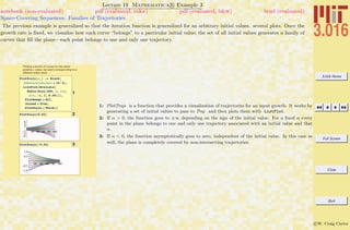
291. 3.016 Home
Full Screen
Close
Quit
c W. Craig Carter
Forward Differencing Methods: Explicit Methods
The previous example is generalized to a discrete change ∆t of a continuous (i.e., time-like) parameter t. The following example
demonstrates the simplest method of numerically solving a simple first-order ODE. first-order explicit finite differencing or
Euler integration.
We begin by approximating the derivative dy/dt at time t with a finite difference approximation:
∆y/∆t = [y(t + ∆t) − y(t)]/[(t + ∆t) − t] (19-4)
We can write down a formula for y(t + ∆t) in terms of current values at t, and thus ‘project y into the future. Suppose we
use fixed small time steps ∆t and the short-hand yn = y(n∆t), yn+1 = y(n∆t + ∆t). Now, we must determine which value
to use for f(y(t)) in dy/dt = f(y): the current value f(yn), the future value f(yn+1), an average value ([f(yn) + f(yn+1)]/2,
or something else. The simplest thing to do is use the current value and then every term (but yn+1 is in terms of n:
yn+1 = yn + ∆tf(yn) (19-5)
This is called explicit forward-differencing or Euler’s method,

292. 3.016 Home
Full Screen
Close
Quit
c W. Craig Carter
Lecture 19 Mathematica R Example 4
First-Order Finite Differences: Method 1 Explicit Finite Differences
notebook (non-evaluated) pdf (evaluated, color) pdf (evaluated, b&w) html (evaluated)
We implement this simple method described in Eq. 19-5 be creating a function which ‘projects’ the current value of y into the future.
Approximate f(y) with f(yi-1);
1
PushMethod1@f_,
8ti_, yi_<, Dt_D :=
8ti + Dt, yi + Dt f@yiD<
2FuncEx@y_D := -Sin@yD
3PushMethod1@
FuncEx, 80, 1<, .01D
4
PushMethod1@FuncEx,
PushMethod1@FuncEx,
80, 1<, .01D, .01D
5Nest@PushMethod1@FuncEx,
Ò, .01D &, 80, 1<, 2D
6
NestList@
PushMethod1@FuncEx,
Ò, .01D &, 80, 1<, 2D
7
NestWhileList@
PushMethod1@FuncEx,
Ò, .01D &, 80, 1<,
HFirst@ÒD < 0.03L &D
1: The function PushMethod1 takes three arguments: argument 1 is a place-holder for another function
that determines how each increment changes (i.e., the function f = dy/ft); argument 2 is the current
value; argument 3 is the discrete forward difference (i.e., ∆t).
2: FuncEx is defined to to pass to sequence-generating functions—it plays the role of f(yn) in Eq. 19-5.
3: For example, this pushes a value {0,1} by ∆t = 0.01 into the future with FuncEx[1].
4: Calling the function, PushMethod1 , recursively on itself (once) pushes the value iteravely into the
future (twice).
5: We can generalize this recursion method by using Nest (Nest[f,x,3] rightarrow f[f[f[x]]]).
However, we must turn PushMethod1 into a function of a single argument, so there is no ambiguity
about which value is being iteratively pushed forward. This is done by creating a Pure Function
version of PushMethod1 . The pure function is indicated by the trailing ampersand, &, and the
# becomes a place holder for the single argument. Thus, Nest[(PushMethod[FuncEx,#,0.01])&,
{0,1}, 2] nests PushMethod1 with fixed first and third arguments (FuncEx and 0.01) on the initial
value {0,1} twice.
6: NestList is another version of Nest, but it stores each increment in a growing list and returns a list
structure.
7: NestListWhile is another version of NestList, but with a switch to tell it when to stop ‘Nesting.’
We use this method to indicate “at what time” the nesting should stop, and not “after how many
nests.” For NestListWhile’ test-argument, we use another pure function: it takes the current value
of {t,y} and tests to see if t is less than 0.03.

293. 3.016 Home
Full Screen
Close
Quit
c W. Craig Carter
Lecture 19 Mathematica R Example 5
Visualizing Trajectories from Explicit Forward Differences
notebook (non-evaluated) pdf (evaluated, color) pdf (evaluated, b&w) html (evaluated)
Examples of the explicit forward differencing function PushMethod1 called recursively with NestListWhile are illustrated. An example
of Numerical Instability appears.
A
A Function PlotM1, taking
arguments for a and initial condition
is used with NestListWhile and
ListPlot to produce graphics with a
red line and green points.
2PlotM1@0.1, 1D
3PlotM1@1.5, 1D
A: PlotM1 is defined which takes a first argument for a time-step, and a second argument is y0. It
uses ListPlot to create a trajectory, and show line segments between the computed points. (The
definition is suppressed in class-notes, it is available via the links given above)
2: Here is an example of a stable numerical integration of a first-order ODE. We have not evaluated
how accurate the numerical algorithm is, but only that it is well-behaved.
3: Using a larger time-step, we can see that the algorithm is becoming less well-behaved. This introduces
the concept maximum stable time-step.

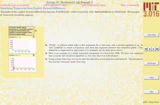
294. 3.016 Home
Full Screen
Close
Quit
c W. Craig Carter
Forward Differencing Methods: Implicit Methods
As in the implicit method, we begin by approximating the derivative dy/dt at time t with a finite difference approximation:
∆y/∆t = [y(t + ∆t) − y(t)]/[(t + ∆t) − t] (19-6)
However, in this case we will use the expected future value, yn+1 as the argument to f(y).
yn+1 = yn + ∆tf(yn+1)
= yn + ∆t f(yn) +
df
dy yn
(yn+1 − yn)
(19-7)
Because yn+1 appears on both sides, we have to solve for it (this is the implicit step),
yn+1 =
yn + ∆t(f(yn) − df
dy yn
yn)
1 − ∆t df
dy yn
(19-8)
This is called implicit forward-differencing.

295. 3.016 Home
Full Screen
Close
Quit
c W. Craig Carter
Lecture 19 Mathematica R Example 6
First-Order Finite Differences: Method 1 Explicit Finite Differences
notebook (non-evaluated) pdf (evaluated, color) pdf (evaluated, b&w) html (evaluated)
We implement this implicit method described in Eq. 19-8
Approximate f(y) with f(yi !); then solving the
finite difference equation above,
yi = yi-1 + Dt [f(yi ) ].
So, yi = yi-1 + Dt (f(yi ) + f'(yi-1)dy)
yi = yi-1 + Dt (f(yi ) + f'(yi-1)(yi - yi-1) )
yi = Hyi-1 - Dt [f(yi-1) - f'(yi-1)yi-1])/
(1 - Dt f'(yi-1) )
1
PushMethod2@f_,
df_, 8ti_, yi_<,
Dt_D := 8ti + Dt,
Hyi + HDt Hf@yiD -
df@yiD yiLLL ê
H1 - Dt df@yiDL<
2
dFuncEx@y_D :=
Evaluate@D@FuncEx@yD, yDD
3
NestList@
PushMethod2@FuncEx,
dFuncEx, Ò, 0.1D &,
80, 1<, 3D
A
We define a function, PlotM2, which
takes arguments Dt and
InitialCondition and then uses
ListPlot with Blue lines and Gray
points.
1: PushMethod2 implements the implicit differencing strategy. However, we must also provide this
method with a function representing the derivative of f.
2: We define the derivative function, but use Evaluate on the right-hand side of the delayed assignment
(:=) so that the derivative operator D is not called each time the function is used.
3: We can use the Nest-family of functions as before.
A: A function to plot the implicit function results is defined for comparison to the explicit method.

296. 3.016 Home
Full Screen
Close
Quit
c W. Craig Carter
Lecture 19 Mathematica R Example 7
Comparison of Implicit and Explicit Methods
notebook (non-evaluated) pdf (evaluated, color) pdf (evaluated, b&w) html (evaluated)
We plot the results from the two different time-stepping methods and show that the implicit method is more stable. We still have not
evaluated the accuracy of either method.
1
Show@PlotM1@0.1, 1D,
PlotM2@0.1, 1D, PlotRange Ø
880, 10<, 80, 1<<D
2
Show@PlotM1@1.5, 1.0D,
PlotM2@1.5, 1.0D,
PlotRange Ø
880, 10<, 8-0.5, 1<<D
Method 2 will fail if the step size is increased
to 2
1: With a time step of ∆t = 0.1, the two methods give results that are barely discernible. This gives
us confidence in the hypothesis that the solutions are also accurate at this time step.
2: At larger time steps, the implicit method is more well-behaved. However, if the step size is made a
little larger, both methods will become unstable.

297. 3.016 Home
Full Screen
Close
Quit
c W. Craig Carter
Geometrical Interpretation of Solutions
The relationship between a function and its derivatives for a first-order ODE,
F(
dy(x)
dx
, y(x), x) = 0 (19-9)
can be interpreted as a level set formulation for a two-dimensional surface embedded in a three-dimensional space with
coordinates (y , y, x). The surface specifies a relationship that must be satisfied between the three coordinates.
If y (x) can be solved for exactly,
dy(x)
dx
= f(x, y) (19-10)
then y (x) can be thought of as a height above the x-y plane.
For a very simple example, consider Newton’s law of cooling which relates the change in temperature, dT/dt, of a body to
the temperature of its environment and a kinetic coefficient k:
dT(t)
dt
= −k(T − To) (19-11)
It is very useful to “non-dimensionalize” variables by scaling via the physical parameters. In this way, a single ODE represents
all physical situations and provides a way to describe universal behavior in terms of the single ODE. For Newton’s law of
cooling, this can be done by defining non-dimensional temperatures and time with Θ = T/To and τ = kt, then if To and k
are constants:
dΘ(τ)
dτ
= (1 − Θ)

298. 3.016 Home
Full Screen
Close
Quit
c W. Craig Carter
Lecture 19 Mathematica R Example 8
Visual Understanding of the Behavior of First-Order ODES
notebook (non-evaluated) pdf (evaluated, color) pdf (evaluated, b&w) html (evaluated)
The surface representation provides a useful way to think about differential equations—much can be inferred about a solution’s be-
havior without computing the solution exactly. This is shown for a simple case of Newton’s law of cooling Equation 19 and an artificial case.
1
ZeroPlane@xmin_,
xmax_, ymin_, ymax_D :=
Graphics3D@8Gray,
Opacity@0.25D, Cuboid@
8xmin, ymin, -.001<,
8xmax, ymax, .001<D<D
2
Show@
Plot3D@1 - Q, 8tau, 0, 2<,
8Q, 0, 2<, AxesLabel Ø
8"t", "Q", "dQêdt"<,
DisplayFunction ->
IdentityD,
ZeroPlane@0, 2, 0, 2DD
1: For first-order ODEs, behavior is dominated by whether the derivative term is positive or negative.
Here, a Graphics3D object is created for a gray-colored opaque horizontal plane (in reality we use
a very thin slab) at z = 0. We will use this function to evaluate when the derivative is positive and
the value is increasing or negative and the value is decreasing.
2: This will create the surface associated with Newton’s law of cooling with the zero plane. This case
is very simple. The sign of the change of Θ depends only the sign of 1 − Θ and therefore dΘ/dt = 0
is the parametric curve (a line in this case) (dΘ/dt = 0, Θ =1 , τ). That is, if Θ = 1 at any time
τ it will stay there at all subsequent times (also, at all previous times as well). Because Θ(τ) will
always increase when Θ < 1 and will always decrease when Θ > 1, the solutions will asymptotically
approach Θ = 1.

299. 3.016 Home
Full Screen
Close
Quit
c W. Craig Carter
Lecture 19 Mathematica R Example 9
Visualizing the Geometry of Flows for First-Order ODES
notebook (non-evaluated) pdf (evaluated, color) pdf (evaluated, b&w) html (evaluated)
By creating vector field which ‘points’ toward subsequent points as inferred from the ODE, we produce a very useful way to understand
solution behavior for a variety of initial conditions, without computing a solution to the ODE. This is shown again for a simple case of
Newton’s law of cooling
Plot the vectorf-ield (dt,dQ) = dt(1, dQ
dt
) !We
can do so by plotting vectors of the form {dt,
dQ} = dt{1, dQ
dt
} which will be proportional to
the vector {1, 1-Q}. This is done as follows:
1
Needs@"VectorFieldPlots`"D;
VectorFieldPlots`VectorFieÖ
ldPlot@81, 1 - Q<,
8tau, 0, 4<,
8Q, -2, 4<, Axes Ø True,
AxesLabel Ø 8"t", "Q"<,
ImageSize Ø FullD
1 2 3 4
t
-2
-1
1
2
3
4
Q
1: The asymptotic behavior can be further visualized by plotting a first-order difference representation
of how the solution is changing in time, i.e, (dτ, dΘ) = dτ
`
1, dΘ
dτ
´
This can be obtained with
VectorFieldPlot from the VectorFieldPlots package. Here the magnitude of the arrows is scaled
by setting dτ = 1.

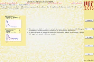
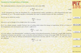
300. 3.016 Home
Full Screen
Close
Quit
c W. Craig Carter
Lecture 19 Mathematica R Example 10
Visualizing the Geometry of Flows for First-Order ODES
notebook (non-evaluated) pdf (evaluated, color) pdf (evaluated, b&w) html (evaluated)
We utilize our visualization methods for intuitive understanding of the behavior of ODES for the case:
dy
dt
= y sin
yt
1 + y + t
Slightly more complicated example:
dy
dt
= y sin(
yt
1 + t +y
),
(dt,dy) = dt(1,ysin
yt
1 + t +y
))
1
Show@Plot3D@
y Sin@ y t ê Ht + y + 1LD,
8t, 0, 10<, 8y, 0, 10<, ,
ZeroPlane@0, 10, 0, 10DDD
2
VectorFieldPlot@
81, y Sin@y t ê Ht + y + 1LD<,
8t, 0, 10<, 8y, 0, 10<D
2 4 6 8 10
t
2
4
6
8
10
y
1: This case can be visualized as well and the behavior can be inferred whether the derivative lies above
or below the zero-plane (i.e., the sign of the derivative). Where dy/dt < 0, y decreases as time
marches forward; thus it moves toward the intersection of the zero plane and the dy/dt-surface. We
see that the slope of the surface evaluated along the curve of intersection determines whether there
is an “attractor-manifold” in the ODE.
2: VectorFieldPlot provides another method to follow a solution trajectories: we plot vectors propor-
tional to dt(1, y sin[yt/(1 + y + t)].

301. 3.016 Home
Full Screen
Close
Quit
c W. Craig Carter
Separable Equations
If a first-order ordinary differential equation F(y , y, x) = 0 can be rearranged so that only one variable, for instance y, appears
on the left-hand-side multiplying its derivative and the other, x, appears only on the right-hand-side, then the equation is
said to be ‘separated.”
g(y)
dy
dx
= f(x)
g(y)dy = f(x)dx
(19-12)
Each side of such an equation can be integrated with respect to the variable that appears on that side:
y
y(xo)
g(η)dη =
x
xo
f(ξ)dξ (19-13)
if the initial value, y(xo) is known. If not, the equation can be solved with an integration constant C0,
g(y)dy = f(x)dx + C0 (19-14)
where C0 is determined from initial conditions. or
y
yinit
g(η)dη =
x
xinit
f(ζ)dζ (19-15)
where the initial conditions appear explicitly.

302. 3.016 Home
Full Screen
Close
Quit
c W. Craig Carter
Lecture 19 Mathematica R Example 11
Using Mathematica R ’s Built-in Ordinary Differential Equation Solver
notebook (non-evaluated) pdf (evaluated, color) pdf (evaluated, b&w) html (evaluated)
Mathematica R has built-in exact and numerical differential equations solvers. DSolve takes a representation of a differential equation
with initial and boundary conditions and returns a solution if it can find one. If insufficient initial or boundary conditions are specified,
then “integration constants” are added to the solution.
1
dsol = DSolve@
8y'@tD == FuncEx@y@tDD<,
y@tD, tD
99y@tD Ø 2 ArcTanA‰-t+C@1D
E==
2
dsol = DSolve@
8y'@tD == FuncEx@y@tDD,
y@0D ã 1<, y@tD, tD
::y@tD Ø 2 ArcTanB‰-t
TanB
1
2
FF>>
The next statement extracts y (x) for plotting ..
3
ExactPlot =
Plot@ y@tD ê. dsol,
8t, 0, 10<, PlotStyle Ø
8Thick, Darker@CyanD<,
PlotRange Ø AllD
2 4 6 8 10
0.2
0.4
0.6
0.8
1.0
1: DSolve operates like Solve . It takes a list of equations containing symbolic derivatives, the function
to be solved for, and the dependent variable. In this case, the general solution of the example we used
for finite differencing examples: dy(x)
dx
= FuncEx [y] DSolve returns a list of rules. The solutions
are be obtained by applying the rules (i.e., y[x]/.dsol). The solution will depend on an integration
constant(s) in general. Mathematica R uses the symbols C[1],C[2],etc as place-holders for the
integration constants.
2: If additional If more constraints (i.e., equations) are provided, then (provided a solution exists) the
integration constant is determined as well. This is the exact solution to what we were numerically
approximating above.
3: The solution is plotted by turning the “solution rule” into a plot-table y[t] Flatten. The plot is
stored as a graphics object ExactPlot.

303. 3.016 Home
Full Screen
Close
Quit
c W. Craig Carter
Lecture 19 Mathematica R Example 12
Comparision of Exact Solutions to Finite Difference Methods
notebook (non-evaluated) pdf (evaluated, color) pdf (evaluated, b&w) html (evaluated)
We compare the plots of implicit, explicit finite differencing to the exact solution obtained by DSolve.
1
Show@PlotM1@0.1, 1D,
PlotM2@0.1, 1D,
ExactPlot, PlotRange Ø
880, 10<, 80, 1<<D
2
Show@PlotM1@1.5, 1D,
PlotM2@1.5, 1D,
ExactPlot, PlotRange Ø
880, 10<, 8-0.25, 1<<D
1: To see how finite differencing compares to the exact solution, we plot all three trajectories together.
The less-stable explicit method is more accurate for intermediate values of t.
2: This shows the comparison at larger time steps.

304. 3.016 Home
Full Screen
Close
Quit
c W. Craig Carter
While the accuracy of the first-order differencing scheme can be determined by comparison to an exact solution, the question
remains of how to establish accuracy and convergence with the step-size δ for an arbitrary ODE. This is a question of primary
importance and studied by Numerical Analysis.

305. 3.016 Home
Full Screen
Close
Quit
c W. Craig Carter
Lecture 19 Mathematica R Example 13
Using Mathematica R ’s Differential Equation Solver on a First-Order ODE: Less Trivial Example
notebook (non-evaluated) pdf (evaluated, color) pdf (evaluated, b&w) html (evaluated)
We solve y (x) + xy(x) = 0 for a ‘strange’ condition y (5) = 1 and plot the solution.
1
dsol = DSolve@
y'@xD + x * y@xD ã 0,
y@xD, xD
Boundary conditions other than y[0]:
2
dsol = DSolve@
8y'@xD + Sin@xD * y@xD ã
0, y'@5D ã 1<, y@xD, xD
99y@xD Ø -‰-Cos@5D+Cos@xD
Csc@5D==
3
GraphicsRow@
8p = Plot@y@xD ê. dsol,
8x, 0, 10<,
PlotStyle Ø ThickD,
Show@p, PlotRange Ø
880, 6<, 80, 6<<,
AspectRatio Ø 1D<D
0 2 4 6 8 10
0.0
0.5
1.0
1.5
2.0
0 1 2 3 4 5 6
0
1
2
3
4
5
6
1: This demonstrates the use of DSolve, because we have not supplied enough conditions to determine
the solution exactly, Mathematica R introduces all the undetermined constants of integration. In
this case, there is only one undetermined constant.
2: Here, the solution is required to have a slope of unity at x = 5. If such a value is possible, then
Mathematica R will compute the corresponding value of C[1].
3: This demonstrates how to extract the solution and plot it. It is plotted a second time with the same
y and x scales so we can see that the slope is indeed one at x = 5.

306. 3.016 Home
Full Screen
Close
Quit
c W. Craig Carter
Nov. 7 2007
Lecture 20: Linear Homogeneous and Heterogeneous ODEs
Reading:
Kreyszig Sections: 1.4, 1.5 (pages19–25, 26–32)
Ordinary Differential Equations from Physical Models
In engineering and physics, modeling physical phenomena is the means by which technological and natural phenomena are
understood and predicted. A model is an abstraction of a physical system, often with simplifying assumptions, into a
mathematical framework. Every model should be verifiable by an experiment that, to the greatest extent possible, satisfies
the approximations that were used to obtain the model.
In the context of modeling, differential equations appear frequently. Learning how to model new and interesting systems is
a learned skill—it is best to learn by following a few examples. Grain growth provides some interesting modeling examples
that result in first-order ODES.
Grain Growth
In materials science and engineering, a grain usually refers a single element in an ensemble that comprises a polycrystal. In a
single phase polycrystal, a grain is a contiguous region of material with the same crystallographic orientation. It is separated
from other grains by grain boundaries where the crystallographic orientation changes abruptly.
A grain boundary contributes extra free energy to the entire system that is proportional to the grain boundary area. Thus,
if the boundary can move to reduce the free energy it will.

307. 3.016 Home
Full Screen
Close
Quit
c W. Craig Carter
Consider simple, uniformly curved, isolated two- and three-dimensional grains.
Figure 20-18: Illustration of a two-dimensional isolated circular grain and a three-dimensional
isolated spherical grain. Because there is an extra energy in the system ∆G2D = 2πRγgb and
∆G3D = 4πR2γgb, there is a driving force to reduce the radius of the grain. A simple model
for grain growth is that the velocity (normal to itself) of the grain boundary is vgb = Mgbγgbκ
where Mgb is the grain boundary mobility and κ is the mean curvature of the boundary. The
normal velocity vgb is towards the center of curvature.
A relevant question is “how fast will a grain change its size assuming that grain boundary migration velocity is proportional
to curvature?”
For the two-dimensional case, the rate of change of area can be formulated by considering the following illustration.

308. 3.016 Home
Full Screen
Close
Quit
c W. Craig Carter
vn
!A =vn!tds
ds
Figure 20-19: A segment of a grain boundary moving with normal velocity vn will move a
distance vn∆t in a short time ∆t. The motion will result in a change of area −∆A for the
shrinking grain. Each segment, ds, of boundary contributes to the loss of area by ∆A =
−vn∆tds.
Because for a circle, the curvature is the same at each location on the grain boundary, the curvature is uniform and vn =
Mgbκgbγgb = Mgbγgb/R. Thus
dA
dt
= −Mgbγgb
1
R
2πR = −2πMgbγgb (20-1)
Thus, the area of a circular grain changes at a constant rate, the rate of change of radius is:
dA
dt
=
dπR2
dt
= 2πR
dR
dt
= −2πMgbγgb (20-2)
which is a first-order, separable ODE with solution:
R2
(t) − R2
(t = 0) = −2Mgbγgbt (20-3)
For a spherical grain, the change in volume ∆V due to the motion of a surface patch dS in a time ∆t is ∆V = vn∆t dS. The
curvature of a sphere is
κsphere =
1
R
+
1
R
(20-4)

309. 3.016 Home
Full Screen
Close
Quit
c W. Craig Carter
Therefore the velocity of the interface is vn = 2Mgbγgb/R. The rate of change of volume due to the contributions of each
surface patch is
dV
dt
= −Mgbγgb
2
R
4πR2
= −8πMgbγgbR == −4(6π2
)1/3
MgbγgbV 1/3
(20-5)
which can be separated and integrated:
V 2/3
(t) − V 2/3
(t = 0) = −constant1t (20-6)
or
R2
(t) − R2
(t = 0) = −constant2t (20-7)
which is the same functional form as derived for two-dimensions.
The problem (and result) is more interesting if the grain doesn’t have uniform curvature.
Figure 20-20: For a two-dimensional grain with non-uniform curvature, the local normal velocity
(assumed to be proportional to local curvature) varies along the grain boundary. Because the
motion is in the direction of the center of curvature, the velocity can be such that its motion
increases the area of the interior grain for some regions of grain boundary and decreases the
area in other regions.
However, it can still be shown that, even for an irregularly shaped two-dimensional grain, A(t) − A(t = 0) = −(const)t.

310. 3.016 Home
Full Screen
Close
Quit
c W. Craig Carter
Integrating Factors, Exact Forms
Exact Differential Forms
In classical thermodynamics for simple fluids, expressions such as
dU =TdS − PdV
=
∂U
∂S V
dS +
∂U
∂V S
dV
=δq + δw
(20-8)
represent the differential form of the combined first and second laws of thermodynamics. If dU = 0, meaning that the
differential Eq. 20-8 is evaluated on a surface for which internal energy is constant, U(S, V ) = const, then the above equation
becomes a differential form
0 =
∂U
∂S V
dS +
∂U
∂V S
dV (20-9)
This equation expresses a relation between changes in S and changes in V that are necessary to remain on the surface
U(S, V ) = const.
Suppose the situation is turned around and you are given the first-order ODE
dy
dx
= −
M(x, y)
N(x, y)
(20-10)
which can be written as the differential form
0 = M(x, y)dx + N(x, y)dy (20-11)
Is there a function U(x, y) = const or, equivalently, is it possible to find a curve represented by U(x, y) = const?
If such a curve exists then it depends only on one parameter, such as arc-length, and on that curve dU(x, y) = 0.

311. 3.016 Home
Full Screen
Close
Quit
c W. Craig Carter
The answer is, “Yes, such a function U(x, y) = const exists if an only if M(x, y) and N(x, y) satisfy the Maxwell relations”
∂M(x, y)
∂y
=
∂N(x, y)
∂x
(20-12)
Then if Eq. 20-12 holds, the differential form Eq. 20-11 is called an exact differential and a U exists such that dU = 0 =
M(x, y)dx + N(x, y)dy.
Integrating Factors and Thermodynamics
For fixed number of moles of ideal gas, the internal energy is a function of the temperature only, U(T)−U(To) = CV (T −To).
Consider the heat that is transferred to a gas that changes it temperature and volume a very small amount:
dU =CV dT = δq + δw = δq − PdV
δq = CV dT + PdV
(20-13)
Can a Heat Function q(T, V ) = constant be found?
To answer this, apply Maxwell’s relations.
Homogeneous and Heterogeneous Linear ODES
A linear differential equation is one that does not contain any powers (greater than one) of the function or its derivatives.
The most general form is:
Q(x)
dy
dx
+ P(x)y = R(x) (20-14)
Equation 20-15 can always be reduced to a simpler form by defining p = P/Q and r = R/Q:
dy
dx
+ p(x)y = r(x) (20-15)

312. 3.016 Home
Full Screen
Close
Quit
c W. Craig Carter
If r(x) = 0, Eq. 20-15 is said to be a homogeneous linear first-order ODE; otherwise Eq. 20-15 is a heterogeneous linear
first-order ODE.
The reason that the homogeneous equation is linear is because solutions can superimposed—that is, if y1(x) and y2(x) are
solutions to Eq. 20-15, then y1(x)+y2(x) is also a solution to Eq. 20-15. This is the case if the first derivative and the function
are themselves linear. The heterogeneous equation is also called linear in this case, but it is important to remember that
sums and/or multiples of heterogeneous solutions are also solutions to the heterogeneous equation.
It will be demonstrated below (directly and with a Mathematica R example) that the homogeneous equation has a solution
of the form
y(x) = const e−
R
p(x)dx
(20-16)
To show this form directly, the homogeneous equation can be written as
dy
dx
= −p(x)y
Dividing each side through by through by y and integrate:
dy
y
= log y = − p(x)dx + const
which has solution
y(x) = conste−
R
p(x)dx
For the case of the heterogeneous first-order ODE, A trick (or, an integrating factor which amounts to the same thing) can
be employed. Multiply both sides of the heterogeneous equation by e
R
p(x):12
exp
x
a
p(z)dz
dy(x)
dx
+ exp
x
a
p(z)dz p(x)y(x) = exp
x
a
p(z)dz r(x) (20-17)
Notice that the left-hand-side can be written as a derivative of a simple expression
exp
x
a
p(z)dz
dy(x)
dx
+ exp
x
a
p(z)dz p(x)y(x) =
d
dx
exp
x
a
p(z)dz y(x) (20-18)
12
The statistical definition of entropy is S(T, V ) = k log Ω(U(T, V )) or Ω(U(T, V )) = exp(S/k). Entropy plays the role of integrating factor.

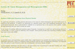
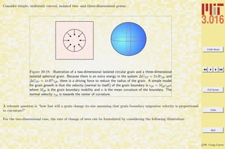
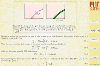
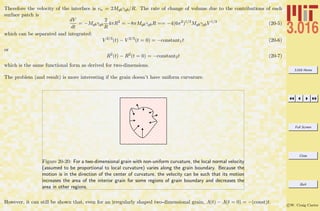
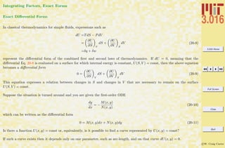
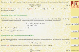
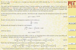
313. 3.016 Home
Full Screen
Close
Quit
c W. Craig Carter
therefore
d
dx
exp
x
a
p(z)dz y(x) = exp [p(x)] r(x) (20-19)
which can be integrated and then solved for y(x):
y(x) = exp −
x
a
p(z)dz y(x = a) +
x
a
r(z) exp
z
a
p(η)dη dz (20-20)

314. 3.016 Home
Full Screen
Close
Quit
c W. Craig Carter
Lecture 20 Mathematica R Example 1
Solutions to the General Homogeneous Linear First-Order ODE
notebook (non-evaluated) pdf (evaluated, color) pdf (evaluated, b&w) html (evaluated)
The form of Mathematica R ’s solution for Eq. 20 is demonstrated.
1
DSolve@
y'@xD + p@xD y@xD ã 0,
y@xD, xD
::y@xD Ø ‰Ÿ1
x
-p@K@1DD „K@1D
C@1D>>
The dummy integration variables (K[1] in the
above) and any integration constants (C[1]
above) are picked by Mathematica . Mathemat-
ica returns the most general form of homoge-
neous linear first-order solutiion,
2
DSolve@
y'@xD + H2 x + 1L y@xD ã 0,
y@xD, xD
::y@xD Ø ‰-x-x2
C@1D>>
There is an integration constant above, that
will take on a specific value if an additional
condition (such as an initial condition, or a
boundary condition) is specified
3
DSolve@
8y'@xD + H2 x + 1L y@xD ã 0,
y@0D == 4<, y@xD, xD
::y@xD Ø 4 ‰-x-x2
>>
1: DSolve solves the linear homogeneous equation first-order ODE dy/dx + p(x)y = 0. Two variables
are introduced in the solution: one is the ‘dummy-variable’ of the integration in Eq. 20 which
Mathematica R introduces in the form K[N] and an integration constant which is given the form
C[N].
2: Here, a specific p(x) is given, so the dummy variable doesn’t appear if p(ζ) can be integrated sym-
bolically, as in this case for p(ζ) = 2x + 1.
3: Furthermore, if enough boundary conditions are given to solve for the integration constants, then
the C[N] are not needed either.

315. 3.016 Home
Full Screen
Close
Quit
c W. Craig Carter
Lecture 20 Mathematica R Example 2
Solutions to the General Heterogeneous Linear First-Order ODE
notebook (non-evaluated) pdf (evaluated, color) pdf (evaluated, b&w) html (evaluated)
This demonstrates the use of DSolve to find symbolic solutions of heterogeneous linear homogeneous first-order ODEs: Eq. 20-20. We
will see how the homogeneous solution is always part of the sum for a heterogeneous solution.
1
2
DSolve@
y'@xD + p@xD y@xD ã r@xD,
y@xD, xD
::y@xD Ø ‰Ÿ1
x
-p@K@1DD „K@1D
C@1D +
‰Ÿ1
x
-p@K@1DD „K@1D
‡
1
x
‰-Ÿ1
K@2D
-p@K@1DD „K@1D
r@K@2DD
„K@2D>>
The solution is general~two dummy integra-
tion variables and one constant of integration.
3
homsol =
DSolve@y'@xD - y@xD ã 0,
y@xD, xD
hetsol = DSolveA
y'@xD - y@xD ã ‰2 x
,
y@xD, xE
99y@xD Ø ‰x
C@1D==
99y@xD Ø ‰2 x
+ ‰x
C@1D==
1: DSolve solves the general linear heterogeneous equation, dy/dx + p(x)y = r(x), to give the form
Eq. 20-20. Note how the homogeneous solution (i.e., the part that depends on C[1]) is part of the
solution.
2: This is an example for a specific case: p(x) = −1 and r(x) = e2x
. The homogeneous solution is
displayed alongside to reinforce that it is always part of the solution.

316. 3.016 Home
Full Screen
Close
Quit
c W. Craig Carter
Example: The Bernoulli Equation
The linear first-order ODEs always have a closed form solution in terms of integrals. In general non-linear ODEs do not have
a general expression for their solution. However, there are some non-linear equations that can be reduced to a linear form;
one such case is the Bernoulli equation:
dy
dx
+ p(x) y = r(x) ya
(20-21)
Reduction relies on a clever change-of-variable, let u(x) = [y(x)]1−a, then Eq. 20-21 becomes
du
dx
+ (1 − a)p(x) u = (1 − a) r(x) (20-22)
which is a linear heterogeneous first-order ODE and has a closed-form solution.
However, not all non-linear problems can be converted to a linear form. In these cases, numerical methods are required.

317. 3.016 Home
Full Screen
Close
Quit
c W. Craig Carter
Lecture 20 Mathematica R Example 3
Changing Variables in Symbolic Differential Equations
notebook (non-evaluated) pdf (evaluated, color) pdf (evaluated, b&w) html (evaluated)
The Bernoulli equation, Eq. 20-21, is used to demonstrate how to change variables in an ODE.
1
BernoulliEquation =
y'@xD + p@xD y@xD ==
r@xD Hy@xDL^HaL
2yRep = u@xD
1
1-a
DyRep = D@yRep, xD
3
step1 = BernoulliEquation ê.
8y@xD Ø yRep,
y'@xD Ø DyRep<
4step2 = PowerExpand@step1D
5step3 = Simplify@step2D
6BE = Solve@step3, u'@xDD
7uprime = u'@xD ê. BE
8
usol =
u@xD ê. DSolve@u'@xD ã
uprime@@1DD, u@xD, xD
9ysol =
Husol@@1DDL^H1 ê H1 - aLL
10
BernoulliEquation
Simplify@
p@xD ysol + D@ysol, xDD
1: The Bernoulli equation is a non-linear first order ODE, but a series of transformations can turn it
into an equivalent linear form.
2: Symbols for what will be used as replacements for y(x) and its derivative in BernoulliEquation are
defined.
3: For step1, the symbols are used for a rule-replacement.
4: Using the form with replacements, the assumption that all variables are real is employed by using
PowerExpand.
5: Simplify produces an equation for which the right-hand-side is zero; thus assuming that u(x) is not
identically zero, it can be factored out of the equation.
6: Using Solve (n.b, not DSolve) to find u (x) reveals the linear form of Bernoulli’s equation in terms
of the new variable.
7: The rule that is produced by Solve is used to extract the symbolic form of u (x); the symbolic form
of u (x) is assigned to uprime.
8: To extract the solution (usol), we use the rule produced by DSolve on the equation u (x) = usol.
9: The back-transformation is used to find the general solution y(x) to the non-linear form of the
Bernoulli equation (ysol).
10: The solution, ysol, is plugged back into the left-hand-side of the Bernoulli equation and, with
Simplify, is shown to be r(x)ysola
.

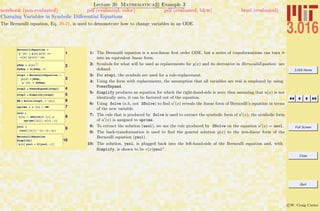
318. 3.016 Home
Full Screen
Close
Quit
c W. Craig Carter
Lecture 20 Mathematica R Example 4
Numerical Solutions to Non-linear First-Order ODEs
notebook (non-evaluated) pdf (evaluated, color) pdf (evaluated, b&w) html (evaluated)
An example of computing the numerical approximation to the solution to a non-linear ODE is presented. The solutions are re-
turned in the forms of a list of replacement rules to InterpolatingFunction. An InterpolatingFunction is a method to use
numerical interpolation to extract an approximation for any point—it works just like a function and can be called on a variable like
InterpolatingFunction[0.2]. In addition to the interpolation table, the definition specifies the domain over which the interpolation is
considered valid.
Mathematica cannot find a direct solution to
the following nonlinear ODE
1
DSolve@
Sin@2 Pi y'@xD^2D ==
y@xD x, y@xD, xD
NDSolve is a numerical method for finding a
solution. An initial condition and the desired
range of solution are required.
2
solution = NDSolve@
8Sin@2 Pi y'@xD^2D ==
y@xD x, y@0D == 1<,
y, 8x, 0, 3.5<D
88y Ø InterpolatingFunction@
880., 3.5<<, <>D<,
8y Ø InterpolatingFunction@
880., 3.5<<, <>D<<
3y@0.5D ê. solution
80.907437, 1.09733 + 0. Â<
4y@PiD ê. solution
80.0524983,
2.50186 - 0.61067 Â<
1: This shows that DSolve cannot find a symbolic solution to sin[2π(y )2
] = y(x)x.
2: Using NDSolve on a non-linear ODE, the solution is returned as a InterpolatingFunction replace-
ment list. Note that there is a warning about “inverse functions” being used to find the solution; this
is because of the sin-function which is causing Mathematica to assume a particular domain. There
may be more solutions than the two that were that were returned as an InterpolatingFunction.
[: 3–4] This demonstrates how the numerical approximation to the non-linear ODE is obtained at
particular values of x.

319. 3.016 Home
Full Screen
Close
Quit
c W. Craig Carter
Lecture 20 Mathematica R Example 5
Plotting Numerical Solutions to Non-linear First-Order ODEs
notebook (non-evaluated) pdf (evaluated, color) pdf (evaluated, b&w) html (evaluated)
This is an example of how to extract plot-table expressions from the rules for InterpolationFunctions that are returned from NDSolve.
1PStyle = 88Red, Thick<,
8Darker@GreenD, Thick<<;
2
PlotVanilla =
Plot@Evaluate@y@xD ê.
solutionD, 8x, 0, 3.5<,
PlotStyle Ø PStyle,
PlotRange Ø 80, 2<,
PlotLabel Ø "Plot"D;
3
PlotReal = Plot@Evaluate@
Re@y@xD ê. solutionDD,
8x, 0, 3.5<, PlotStyle Ø
PStyle, PlotLabel Ø
"Real Part"D;
4
PlotIm = Plot@Evaluate@
Im@y@xD ê. solutionDD,
8x, 0, 3.5<, PlotStyle Ø
PStyle, PlotLabel Ø
"Imaginary Part"D;
5
GraphicsRow@8PlotVanilla,
PlotReal, PlotIm<,
ImageSize Ø SmallD
1: Because solution obtained above is a list containing two rules, two curves will be plotted. Here we
define a short-hand for the expression that will be passed to PlotStyle in the plots below. The first
curve will be red, and the second will be Darker green.
2: Here, Plot is called on the y[x] with replacements defined the rule-set for InterpolatingFunctions,
solution, that was obtained from NDSolve previously. Using Evaluate here immediately creates
a list of length two, and plot recognizes this as two curves to which the PlotStyles can be applied.
If Evaluate were not used, then both curves would be be red.
Plot only produces curves where the numerical value can be represented by a real number; if a
solution has a point where it transforms from real to complex, Plot will show a curve that appears
to end.
3–4: To determine the solution behavior, the real and imaginary parts are extracted with Re and Im.
5: This GraphicsRow indicates the solution behavior: the first solution is real over the domain where
the interpolation is valid; the second solution transforms from real to complex near x = 0.8.

320. 3.016 Home
Full Screen
Close
Quit
c W. Craig Carter
Nov. 9 2007
Lecture 21: Higher-Order Ordinary Differential Equations
Reading:
Kreyszig Sections: 2.1, 2.2 (pages45–52, 53–58)
Higher-Order Equations: Background
For first-order ordinary differential equations (ODEs), F(y (x), y(x), x), one value y(xo) was needed to specify a particular so-
lution. Recall the example in Lecture 19 of a first-order differencing scheme: at each iteration the function grew proportionally
to its current size. In the limit of very small forward differences, the scheme converged to exponential growth.
Now consider a situation in which function’s current rate of growth increases proportionally to two terms: its current rate of
growth and its size.
Change in Value’s Rate of Change + α (the Value) + β (Value’s Rate of Change) = 0
To calculate a forward differencing scheme for this case, let ∆ be the forward-differencing increment.
Fi+2−Fi+1
∆ − Fi+1−Fi
∆
∆
+ αFi + β
Fi+1 − Fi
∆
= 0
and then solve for the “next increment” Fi+2 if Fi+1 and Fi are known.
This indicates that, for second-order equations, two independent values are needed to generate the ‘solution trajectory.’

321. 3.016 Home
Full Screen
Close
Quit
c W. Craig Carter
Lecture 21 Mathematica R Example 1
A Second-Order Forward Differencing Example
notebook (non-evaluated) pdf (evaluated, color) pdf (evaluated, b&w) html (evaluated)
A second order differencing formula is developed for second-order equations. The current value of the right-hand side is used, and
therefore this is an explicit method.
1
ChangePerD@F_, i_, D_D :=
HF@i + 1D - F@iDL ê D
2
ChangeofChangeperD@
F_, i_, D_D :=
Simplify@HChangePerD@
F, i + 1, DD ê D -
ChangePerD@F, i, DDLD
3
DifferenceRelation =
ChangeofChangeperD@
F, i, DD ==
-b ChangePerD@F, i, DD -
a F@iD
4
ForDiffSol = Collect@
Solve@DifferenceRelation,
F@i + 2DD, DD
Replace to find the form of the solution
5ForDiffSolV2 =
ForDiffSol ê. i Ø j - 2
99F@jD Ø
-a D2
F@-2 + jD + F@-1 + jD +
D H-F@-2 + jD + b F@-2 + jD +
F@-1 + jD - b F@-1 + jDL==
1: Changeper∆ is an example of a first-order finite difference approximation to the first derivative.
2: ChangeofChangeper∆ is the second order difference operation, it is obtained by applying the first-
order difference operator twice. Note that two sequential values appear and that the differencing
operator is proportional to 1/∆2
. This is a general feature of high-order difference operators—
with higher difference operations goes, the number of surrounding points required to evaluate the
difference gets larger and larger (e.g., for the second order difference, function values are needed at
three different i compared to two different i for the first-order case.
3: For a particular case of d2
y/dx2
= −αdy/dx−βy, the two difference operators replace the derivatives
and a difference relation can be derived as a function of parameters α and β. We assign the equation
representing the difference relation to DifferenceRelation .
4: The difference operator is derived by solving the difference relation for Fi+2—it will depend on the
immediate last value Fi+1 and that value’s antecedent Fi. Therefore, any value—including the first
one calculated—requires two values to be specified.
5: Typically, the current j–value is expressed in terms of the (j − 1) and (j − 2)–values. This form is
generated by the replacement i → j − 2.

322. 3.016 Home
Full Screen
Close
Quit
c W. Craig Carter
Lecture 21 Mathematica R Example 2
A Second-Order Forward Differencing Example
notebook (non-evaluated) pdf (evaluated, color) pdf (evaluated, b&w) html (evaluated)
Iteration sequences are produced using the explicit differencing operators produced above. A particular example of a second-order
method with constant coefficients is presented.
1
GrowList@ValuesList_List,
D_ , a_ , b_D :=
Module@8Minus1 =
ValuesList@@-1, 2DD,
Minus2 = ValuesList@@-2,
2DD, LastX =
ValuesList@@-1, 1DD<,
Append@ValuesList,
8LastX + D,
2 * Minus1 - Minus2 +
D * Hb * HMinus2 -
Minus1L -
a * D * Minus2L<DD
2InitVals =
880, 1<, 8.001, 1<<;
3result = GrowList@
InitVals, .001, 1, .1D
4result = GrowList@
result, .001, 1, .1D
5
NestWhile@
GrowList@Ò, .001, 1, .1D &,
InitVals,
HLast@ÒD@@1DD < 0.02L &D
1: The difference operator is incorporated in GrowList : a function that grows a list (input as
ValuesList) using a difference ∆ and parameters α and β. The two previous values in the list
become localized variables in a Module function. The Module returns a new list that is created using
Append to place the current value at end of the input list.
2: Because two values are required, a list of size two must be provided. These values could represent
the initial value and the initial value of the derivative.
3: Here is an example of using GrowList once.
4: Using NestWhile the list can be grown iteratively until the first value (i.e., the current value of
xi = xi−1 + ∆) reaches are specified value (here 0.02).

323. 3.016 Home
Full Screen
Close
Quit
c W. Craig Carter
Lecture 21 Mathematica R Example 3
Visualization of Second-Order Forward Differencing
notebook (non-evaluated) pdf (evaluated, color) pdf (evaluated, b&w) html (evaluated)
A second order differencing formula is developed for the case of constant growth and acceleration coefficients.
Visualize results out to x=50 (takes about 24
seconds to visualize )
1
ListPlot@
NestWhile@GrowList@Ò,
.001, 2, .1D &, InitVals,
HLast@ÒD@@1DD < 50L &DD
10 20 30 40 50
-0.5
0.5
1.0
Change parameters for Growth Function (this
example shows that the numerical solution
does not converge to the accurate solution):
2
ListPlot@NestWhile@
GrowList@Ò, 0.01, 2, 0D &,
InitVals,
HLast@ÒD@@1DD < 50L &DD
10 20 30 40 50
-1.5
-1.0
-0.5
0.5
1.0
1.5
1: ListPlot visualizes the results for growth constants α = 2 and β = 0.1. NestWhile operates on
a pure function constructed from GrowList until x = 50. The solution is oscillatory with fixed
frequency, but with exponentially decreasing amplitude. This behavior is correct, although we have
not analyzed the numerical stability or the accuracy of this method.
2: Here is another example with β = 0. With a small enough time step, this should mimic a harmonic
oscillator. The increasing amplitude indicates a numerical inaccuracy at this time-step size.

324. 3.016 Home
Full Screen
Close
Quit
c W. Craig Carter
Linear Differential Equations; Superposition in the Homogeneous Case
A linear differential equation is one for which the function and its derivatives are each linear—that is they appear in distinct
terms and only to the first power. In the case of a homogeneous linear differential equation, the solutions are superposable.
In other words, sums of solutions and their multiples are also solutions.
Therefore, a linear heterogeneous ordinary differential equation can be written as a product of general functions of the
dependent variable and the derivatives for the n-order linear case:
0 = f0(x) + f1(x)
dy
dx
+ f2(x)
d2y
dx2
+ · · · + fn(x)
dny
dxn
= (f0(x), f1(x), f2(x), . . . , fn(x)) · 1,
dy
dx
,
d2y
dx2
, . . . ,
dny
dxn
= f(x) · Dny
(21-1)
The homogeneous nth-order linear ordinary differential equation is defined by f0(x) = 0 in Eq. 21-1:
0 = f1(x)
dy
dx
+ f2(x)
d2y
dx2
+ · · · + fn(x)
dny
dxn
= (0, f1(x), f2(x), · · · , fn(x)) · 1,
dy
dx
,
d2y
dx2
, . . . ,
dny
dxn
= fhom(x) · Dny
(21-2)
Equation 21-1 can always be multiplied by 1/fn(x) to generate the general form:
0 = F0(x) + F1(x)
dy
dx
+ F2(x)
d2y
dx2
+ · · · +
dny
dxn
= (F0(x), F1(x), F2(x), . . . , 1)) · (1,
dy
dx
,
d2y
dx2
, . . . ,
dny
dxn
)
= F(x) · Dny
(21-3)

325. 3.016 Home
Full Screen
Close
Quit
c W. Craig Carter
For the second-order linear ODE, the heterogeneous form can always be written as:
d2y
dx2
+ p(x)
dy
dx
+ q(x)y = r(x) (21-4)
and the homogeneous second-order linear ODE is:
d2y
dx2
+ p(x)
dy
dx
+ q(x)y = 0 (21-5)
Basis Solutions for the homogeneous second-order linear ODE
Because two values must be specified for each solution to a second order equation—the solution can be broken into two basic
parts, each deriving from a different constant. These two independent solutions form a basis pair for any other solution to
the homogeneous second-order linear ODE that derives from any other pair of specified values.
The idea is the following: suppose the solution to Eq. 21-5 is found the particular case of specified parameters y(x = x0) = A0
and y(x = x1) = A1, the solution y(x; A0, A1) can be written as the sum of solutions to two other problems.
y(x; A0, A1) = y(x, A0, 0) + y(x, 0, A1) = y1(x) + y2(x) (21-6)
where
y(x0, A0, 0) = A0 and y(x1, A0, 0) = 0
y(x0, 0, A1) = 0 and y(x1, 0, A1) = A1
(21-7)
from these two solutions, any others can be generated.
The two arbitrary integration constants can be included in the definition of the general solution:
y(x) = C1y1(x) + C1y2(x)
= (C1, C2) · (y1, y2)
(21-8)

326. 3.016 Home
Full Screen
Close
Quit
c W. Craig Carter
Second Order ODEs with Constant Coefficients
The most simple case—but one that results from models of many physical phenomena—is that functions in the homogeneous
second-order linear ODE (Eq. 21-5) are constants:
a
d2y
dx2
+ b
dy
dx
+ cy = 0 (21-9)
If two independent solutions can be obtained, then any solution can be formed from this basis pair.
Surmising solutions seems a sensible strategy, certainly for shrewd solution seekers. Suppose the solution is of the form
y(x) = exp(λx) and put it into Eq. 21-9:
(aλ2
+ bλ + c)eλx
= 0 (21-10)
which has solutions when and only when the quadratic equation aλ2 + λx + c = 0 has solutions for λ.
Because two solutions are needed and because the quadratic equation yields two solutions:
λ+ =
−b +
√
b2 − 4ac
2a
λ− =
−b −
√
b2 − 4ac
2a
(21-11)
or by removing the redundant coefficient by diving through by a:
λ+ =
−β
2
+ (
β
2
)2 − γ
λ− =
−β
2
− (
β
2
)2 − γ
(21-12)
where β ≡ b/a and γ ≡ c/a.

327. 3.016 Home
Full Screen
Close
Quit
c W. Craig Carter
Therefore, any solution to Eq. 21-9 can be written as
y(x) = C+eλ+x
+ C−eλ−x
(21-13)
This solution recreated with a slightly different method in the following Mathematica R example.

328. 3.016 Home
Full Screen
Close
Quit
c W. Craig Carter
Lecture 21 Mathematica R Example 4
Deriving the Solutions to the Homogeneous Linear Second Order ODE with Constant Coefficients
notebook (non-evaluated) pdf (evaluated, color) pdf (evaluated, b&w) html (evaluated)
Even though Mathematica R is able to determine solutions to linear second-order ODEs with constant coefficients directly, it is still
instructive to use Mathematica R to derive these solutions.
1
TheODE@function_, var_D :=
D@function@varD,
8var, 2<D +
b D@function@varD, varD +
g function@varD
2TheODE@y, xD
Guess a solution and substitute it into the left-
hand side of the ODE:
3TheGuess@x_D := Exp@l xD
4TheODE@TheGuess, xD
This will be a solution when the resulting
quadratic expression in l is equal to 0:
5
lSolution = Solve@
TheODE@TheGuess, xD ã 0,
lD
68lMinus, lPlus< =
l ê. lSolution
7
GenSol@x_D :=
C@LPlusD Exp@lPlus xD +
C@LMinusD Exp@lMinus xD
8TheODE@GenSol, zD
9Simplify@TheODE@GenSol, zDD
1–2: TheODE represents the left-hand side of any second-order ODE with constant coefficients—it is
the differential representation of the second-order differencing method that was developed above.
TheODE an argument for the name of the function (i.e., y) and the dependent variable (i.e., x in
y(x)).
3: This will serve as a ‘guess’ of a solution—if we can find λ(s) that satisfy the ODE, then the solution(s)
are determined.
4: The guess is inserted as the first argument to TheODE . The property of the exponential function,
deαx
/dx = d(guess)/dx = αeαx
= αguess will permit factoring of the ‘guessed’ solution.
5: Using Solve with the guess inserted into TheODE will determine solution conditions on λ—this
will be a quadratic equation in λ. The quadratic equation’s solution ensures that, if the solution is
complex, the two λ are complex conjugates.
6: By extraction the solution from the rules returned from Solve, assignments can be made to the two
possible λ.
7: This is the form of the general solution in terms of two arbitrary constants.
8: This should show that the general solution always satisfies the ODE.

329. 3.016 Home
Full Screen
Close
Quit
c W. Craig Carter
Lecture 21 Mathematica R Example 5
Characterizing the Solution Behavior for the Second-Order ODE with Constant Coefficients
notebook (non-evaluated) pdf (evaluated, color) pdf (evaluated, b&w) html (evaluated)
Because the fundamental solution depend on only two parameters β and γ, the behavior (i.e., whether λ
>
< 0 and λ
?
= 0) of all
solutions can be visualized in the γ-β plane.
1
RealsCond =
Reduce@lPlus œ Reals &&
lMinus œ Reals,
8b, g<, RealsD
AThe Complex and Real Domains
BThe Sign of the Real Part of Complex
Solutions
CReal Solutions, Both Positive or
Both Negative
DReal Solutions, Opposite Signs
15
Show@CplexPlot,
RealRootsPos,
MixedRealRoots,
RealRootsNegD
1: Reduce is a function for determining the conditions on parameters (here β and γ assumed to be real
numbers) such that an expression satisfies particular constraints. The results from Reduce will be
used to build up a graphical representation of solution behavior by incremental steps.
A: (Algorithm suppressed in class-notes) RegionPlot is used in conjunction with the results produced
by Reduce to illustrate the domains where the λ are complex and real. The regions are annotated
and saved as a graphic to be concatenated below. This will create a plot that distinguishes two
regions in the γ-β plane: above γ = β2
/4, the λ are real; below, the λ are complex and oscillatory
solutions appear (because exp(r + ıθ) = exp(r)(cos(θ) + ı sin(θ))).
B: The sign of the real part of the complex λ changes at β = 0. Here a graphic and its notation are
created.
C: Using Reduce and RegionPlot in a manner that parallels A, domains for the λ having two real
roots with the same sign are plotted and annotated.
D: Finally, the domain when the λ are real with opposite sign are illustrated.
2: Concatenating all the graphical objects together with Show produces the image that was used to
construct Fig. 21-21.

330. 3.016 Home
Full Screen
Close
Quit
c W. Craig Carter
The behavior of all solutions can be collected into a simple picture:
!
! = "2
4
"
Roots are Complex Conjugates
Positive and Negative
Positive Real Part Negative Real Part
Positive Roots Negative Roots
Roots are Real
Figure 21-21: The behaviors of the linear homogeneous second-order ordinary differential equa-
tion d2y
dx2 + β dy
dx + γy = 0 plotted according the behavior of the solutions for all β and γ.
The case that separates the complex solutions from the real solutions, γ = (β/2)2 must be treated separately, for the case
γ = (β/2)2 it can be shown that y(x) = exp(βx/2) and y(x) = x exp(βx/2) form an independent basis pair (see Kreyszig

331. 3.016 Home
Full Screen
Close
Quit
c W. Craig Carter
AEM, p. 74).
Boundary Value Problems
It has been shown that all solutions to d2y
dx2 + β dy
dx + γy = 0 can be determined from a linear combination of the basis solution.
Disregard for a moment whether the solution is complex or real, and ignoring the special case γ = (β/2)2. The solution to
any problem is given by
y(x) = C+eλ+x
+ C−eλ−x
(21-14)
How is a solution found for a particular problem? Recall that two values must be specified to get a solution—these two values
are just enough so that the two constants C+ and C− can be obtained.
In many physical problems, these two conditions appear at the boundary of the domain. A typical problem is posed like this:
Solve
m
d2y(x)
dx2
+ ν
dy(x)
dx
+ ky(x) = 0 on 0 < x < L (21-15)
subject to the boundary conditions
y(x = 0) = 0 and y(x = L) = 1
or, solve
m
d2y(x)
dx2
+ ν
dy(x)
dx
+ ky(x) = 0 on 0 < x < ∞ (21-16)
subject to the boundary conditions
y(x = 0) = 1 and y (x = L) = 0
When the value of the function is specified at a point, these are called Dirichlet conditions; when the derivative is specified,
the boundary condition is called a Neumann condition. It is possible have boundary conditions that are mixtures of Dirichlet
and Neumann.

332. 3.016 Home
Full Screen
Close
Quit
c W. Craig Carter
Lecture 21 Mathematica R Example 6
Determining Solution Constants from Boundary Values
notebook (non-evaluated) pdf (evaluated, color) pdf (evaluated, b&w) html (evaluated)
Here is an example of taking the general solution with undetermined constants and using boundary conditions to determine a specific
solution.
Second order ODEs require that two condi-
tions to generate a particular solution.
1GenSol@xD
Example of y(0) = 0 and y(L)=1:
2
SolutionOne =
Solve@8GenSol@0D == 0,
GenSol@LD == 1<,
8C@LPlusD, C@LMinusD<D
Write the resulting solution:
3
SpecificSolutionOne =
Simplify@
GenSol@xD ê. SolutionOneD
Second example: y(0) = 1 and y'(0)=0
4DGen = D@GenSol@xD, xD
Now the constants CPlus and CMinus are
found by solving:
5
SolutionTwo =
Solve@8GenSol@0D ã 1,
HDGen ê. x Ø 0L ã 0<,
8C@LPlusD, C@LMinusD<D
6
SpecificSolutionTwo =
Simplify@
GenSol@xD ê. SolutionTwoD
1: GenlSol is the solution to y + βy + γy = 0 with undetermined constants Cplus and Cminus that
we derived above.
2: To demonstrate the method of using boundary conditions for a particular solution the boundary
conditions, we use the example y(0) = 0 and y(L) = 1. Solve is used for the two conditions to find
a rule-set for solutions in terms of the general-solution constants.
3: The form of the particular solution is obtained by back-substituting the solution for the constants
into the general solution.
4: For application of a Neumann condition, the symbolic form of the derivative is required.
5–6: The particular solution for boundary conditions y (0) = y(0) = 0 is obtained by inserting these
equations into Solve and subsequent replacement into the general solution.

333. 3.016 Home
Full Screen
Close
Quit
c W. Craig Carter
Fourth Order ODEs, Elastic Beams
Another linear ODE that has important applications in materials science is that for the deflection of a beam. The beam
deflection y(x) is a linear fourth-order ODE:
d2
dx2
EI
d2y(x)
dx2
= w(x) (21-17)
where w(x) is the load density (force per unit length of beam), E is Young’s modulus of elasticity for the beam, and I is the
moment of inertia of the cross section of the beam:
I =
A×−sect
y2
dA (21-18)
is the second-moment of the distribution of heights across the area.
If the moment of inertia and the Young’s modulus do not depend on the position in the beam (the case for a uniform beam
of homogeneous material), then the beam equation becomes:
EI
d4y(x)
dx4
= w(x) (21-19)
The homogeneous solution can be obtained by inspection—it is a general cubic equation yhomog(x) = C0 +C1x+C2x2 +C3x3
which has the four constants that are expected from a fourth-order ODE.
The particular solution can be obtained by integrating w(x) four times—if the constants of integration are included then the
particular solution naturally contains the homogeneous solution.
The load density can be discontinuous or it can contain Dirac-delta functions Foδ(x−xo) representing a point load Fo applied
at x = xo.
It remains to determine the constants from boundary conditions. The boundary conditions can be determined because each
derivative of y(x) has a specific meaning as illustrated in Fig. 21-22.

334. 3.016 Home
Full Screen
Close
Quit
c W. Craig Carter
slope: dy
dx
d4y
dx4 = w
EI
w(x)
S
load density
stiffness
d3y
dx3 = S
EI
shear force
stiffness d2y
dx2 = M
EI
bending moment
stiffness
S M M
Figure 21-22: The shape of a loaded beam is determined by the loads applied over its length
and its boundary conditions. The beam curvature is related to the local moment (imagine two
handles rotated in opposite directions on a free beam) divided by the effective beam stiffness.
Shear forces are related to the rate of change of moment along the beam.
(Polar Bear Photo Art Wolfe The Zone Network
http://classic.mountainzone.com/climbing/greenland/graphics/polar-bear.html )
There are common loading conditions that determine boundary conditions:

335. 3.016 Home
Full Screen
Close
Quit
c W. Craig Carter
Free No applied moments or applied shearing force:
M =
d2y
dx2
boundary
= 0
S =
d3y
dx3
boundary
= 0
Point Loaded local applied moment, displacement specified.
M =
d2y
dx2
boundary
= Mo
y(x)|boundary = yo
Clamped Displacement specified, slope specified
dy
dx boundary
= so
y(x)|boundary = yo

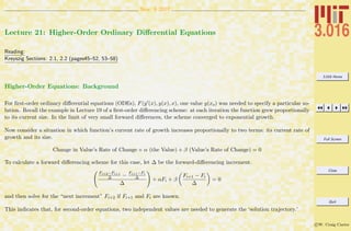
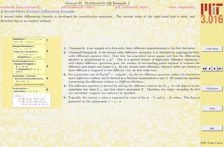
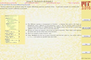
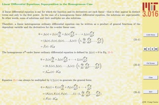
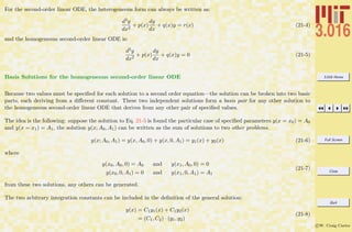
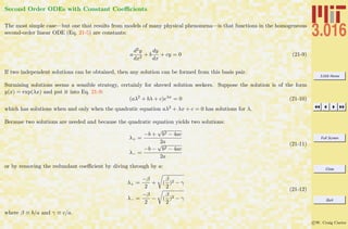
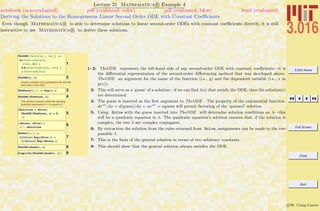
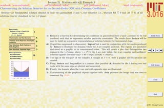
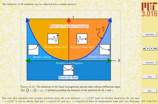
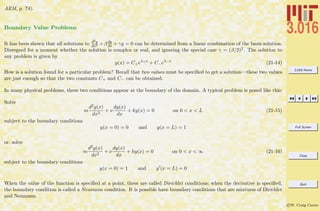
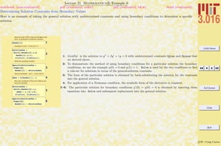
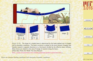
336. 3.016 Home
Full Screen
Close
Quit
c W. Craig Carter
Lecture 21 Mathematica R Example 7
A Function to Solve Beam Deflections for Common Boundary Conditions
notebook (non-evaluated) pdf (evaluated, color) pdf (evaluated, b&w) html (evaluated)
A function for solving and visualizing the deflection of a uniform beam is developed for typical boundary conditions and load distributions
Set up the ODE solution (we will specify a unit
beam stiffness) EI = 1
1
BeamEquation@y_ , x_ ,
w_, BC1_ , BC2_D :=
DSolve@8y ''''@xD ==
w@xD, BC1, BC2<,
y@xD, xD êê Flatten
AFunctions for Typical Boundary
Conditions and Beam Loading
10
BeamEquation@y, x,
noload, Clamp@y, 0, 0, 0D,
Knob@y, 1, -.1, 0DD
9y@xD Ø -0.15 x2
+ 0.05 x3
=
1: BeamEquation takes arguments for the (unknown) deflection y and its dependent argument x,
a loading density w(x), and boundary condition lists BC1 and BC2, and uses DSolve to return
replacement rules for a particular solution to the beam deflection equation (i.e., d4
y/dx4
= w(x)).
A: The boundary conditions are defined as functions that return lists of equations for many common
conditions (definitions suppressed in class-notes):
i Clamp [y,x,position,slope] fixed position and derivative at a specified point x of y.
ii Knob [y,x,position,moment] fixes the position and the moment at specified point.
iii FreeBeam [y,x] specifies that the beam is free to move at a specified point.
Particular types of applied loading functions (w(x)) are defined.
i noload [x]: no distributed load.
ii unitload [x]: unit (uniform) distributed load (i.e. 1 load unit/length).
iii midload [x] specifies that a (downward) load of magnitude 10 is applied at x = 1/2.
iv boxload [x,position, width, magnitude] specifies a uniform distributed load with magnitude
over the domain (position - width/2 < x < position + width/2)
v linearload [x] specifies a linearly increasing load is applied, starting at -250 at x = 0 and increasing
to +250 at x = 1.
10: An example of the use of BeamEquation with a clamp and a know is demonstrated.

337. 3.016 Home
Full Screen
Close
Quit
c W. Craig Carter
Lecture 21 Mathematica R Example 8
Visualization of Beam Deflections
notebook (non-evaluated) pdf (evaluated, color) pdf (evaluated, b&w) html (evaluated)
A graphical function is produced to visualize beam deflections for the specified boundary conditions and distributed loads.
1
Plot@Evaluate@
y@xD ê. BeamEquation@
y, x, noload,
Clamp@y, 0, 0, 0D,
Knob@y, 1, -.25, 0DD
D, 8x, 0, 1<D
ABeamViz: Visualization Function
3
BeamViz@unitload,
Clamp@y, 0, 0, 0D,
FreeBeam@y, 1DD
4
BeamViz@linearload,
Knob@y, 0, 0, 0D,
Knob@y, 1, 0, 0DD
5
BeamViz@boxload@Ò,
3 ê 4, 1 ê 8, -500D &,
Clamp@y, 0, 0, 0D,
Clamp@y, 1, 0, 0DD
0.2 0.4 0.6 0.8 1.0
-0.4
-0.2
0.2
0.4
1: To plot the beam deflection, the solution condition is used as rule for replacement to y(x)
A: The function BeamViz collects the solution with the visualization for beams of unit normalized
length, and uniform normalized stiffness EI.
3–4: These are examples of different loading conditions and boundary conditions are visualized as exam-
ples of BeamViz .
5: In this case, we have to force the loading condition w(x) to be a function of a single variable. Because
boxload takes four arguments, it is necessary to use it to construct a pure function.

338. 3.016 Home
Full Screen
Close
Quit
c W. Craig Carter
Lecture 21 Mathematica R Example 9
A Gratuitous Animations of Deflections of a Diving Board
notebook (non-evaluated) pdf (evaluated, color) pdf (evaluated, b&w) html (evaluated)
A diving board can be approximated as a beam of uniform stiffness which is cantilevered at one end, and has an adjustable pin near its
center. We work out a solution and visualization for a diver walking out on a diving board with the pin fixed at the center.
We wish to simulate the deflection of a diving
board as a diver walks toward the end. A
diving board may be modeled as beam with
constant cross-section. The boundary condi-
tions are that the board is clamped at the
beginning; has a pivot located somewhere
near the center; and the "diving" end . For
"competitive" diving boards, the pivot point is
adjustable. Here we fix the pivot at x=1/2.
This next function is a silly little graphic for the
walking diver.
AGraphics Functions for Animating
Board and Diver
: >
A: (Solution and Algorithm Suppressed) We start by defining a set of graphics that take a single argu-
ment to represent the diver, the argument is designed to make the diver appear to be walking.
The solution to this deflection of the diving board is not trivial. The diver is modeled as a point
load. The board is modeled as a piecewise solution for two beams that share a common boundary
condition. We will need to match boundary conditions at the pin. The method is to find a solution
in terms of an arbitrary coefficient, and then solve for the instance of that coefficient that makes the
board deflection continuous.
If the diver is located between the cantilever and the pin, then the deflection in this region is
determined with simple clamp and pin boundary conditions and the DiracDelta function for the
distributed load. From this solution, the slope at the mid-point is calculated and this value is used
as one of the boundary condition between the pin and the free-end.
If the diver is located between the pin and the free-end, the the slope at the pin is an undermined
constant first in this region and then in the region between the cantilever and the pin. Solve is
used to match the slope at the pin, and that solution is applied to the previously obtained solutions
(i.e., the solutions from DSolve.
Piecewise is used in the definition of the solution-function that is returned.
Manipulate is used to specify the position of the diver.

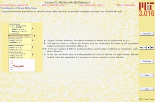
339. 3.016 Home
Full Screen
Close
Quit
c W. Craig Carter
Nov. 14 2007
Lecture 22: Differential Operators, Harmonic Oscillators
Reading:
Kreyszig Sections: 2.3,2.4, 2.7 (pages59–60, 61–69, 78–83)
Differential Operators
The idea of a function as “something” that takes a value (real, complex, vector, etc.) as “input” and returns “something else”
as “output” should be very familiar and useful.
This idea can be generalized to operators that take a function as an argument and return another function.
The derivative operator operates on a function and returns another function that describes how the function changes:
D[f(x)] =
df
dx
D[D[f(x)]] = D2
[f(x)] =
d2f
dx2
Dn
[f(x)] =
dnf
dxn
D[αf(x)] =αD[f(x)]
D[f(x) + g(x)] =D[f(x)] + D[g(x)]
(22-1)
The last two equations above indicate that the “differential operator” is a linear operator.

340. 3.016 Home
Full Screen
Close
Quit
c W. Craig Carter
The integration operator is the right-inverse of D
D[I[f(x)]] = D[ f(x)dx] (22-2)
but is only the left-inverse up to an arbitrary constant.
Consider the differential operator that returns a constant multiplied by itself
Df(x) = λf(x) (22-3)
which is another way to write the the homogenous linear first-order ODE and has the same form as an eigenvalue equation.
In fact, f(x) = exp(λx), can be considered an eigenfunction of Eq. 22-3.
For the homogeneous second-order equation,
D2
+ βD − γ [f(x)] = 0 (22-4)
It was determined that there were two eigensolutions that can be used to span the entire solution space:
f(x) = C+eλ+x
+ C−eλ−x
(22-5)
Operators can be used algebraically, consider the inhomogeneous second-order ODE
aD2
+ bD + c [y(x)] = x3
(22-6)
By treating the operator as an algebraic quantity, a solution can be found13
y(x) =
1
aD2 + bD + c
[x3
]
=
1
c
−
b
c2
D +
b2 − ac
c3
D2
−
b(b2 − 2ac)
c3
D3
+ O(D4
) x3
=
x3
c
−
3bx2
c2
+
6(b2 − ac)x
c3
−
6b(b2 − 2ac)
c3
(22-7)
13
This method can be justified by plugging back into the original equation and verifying that the result is a solution.

341. 3.016 Home
Full Screen
Close
Quit
c W. Craig Carter
which solves Eq. 22-6.
The Fourier transform is also a linear operator:
F[f(x)] =g(k) =
1
√
2π
∞
−∞
f(x)eıkx
dx
F−1
[g(k)] =f(x) =
1
√
2π
∞
−∞
g(k)e−ıkx
dk
(22-8)
Combining operators is another useful way to solve differential equations. Consider the Fourier transform, F, operating on
the differential operator, D:
F[D[f]] =
1
√
2π
∞
−∞
df(x)
dx
eikx
dx (22-9)
Integrating by parts,
=
1
√
2π
f(x) |x=∞
x=−∞ −
ık
√
2π
∞
−∞
f(x)eikx
dx (22-10)
If the Fourier transform of f(x) exists, then typically14 limx→±∞ f(x) = 0. In this case,
F[D[f]] = −ikF[f(x)] (22-11)
and by extrapolation:
F[D2
[f]] = −k2
F[f(x)]
F[Dn
[f]] = (−1)n
ın
kn
F[f(x)]
(22-12)
Operational Solutions to ODEs
Consider the heterogeneous second-order linear ODE which represent a forced, damped, harmonic oscillator that will be
discussed later in this lecture.
M
d2y(t)
dt2
+ V
dy(t)
dt
+ Ksy(t) = cos(ωot) (22-13)
14
It is not necessary that limx→±∞ f(x) = 0 for the Fourier transform to exist but it is satisfied in most every case. The condition that the
Fourier transform exists is that
R ∞
−∞
|f(x)|dx exists and is bounded.

342. 3.016 Home
Full Screen
Close
Quit
c W. Craig Carter
Apply a Fourier transform (mapping from the time (t) domain to a frequency (ω) domain) to both sides of 22-13:
F[M
d2y(t)
dt2
+ V
dy(t)
dt
+ Ksy(t)] = F[cos(ωot)]
−Mω2
F[y] − ıωV F[y] + KsF[y] =
π
2
[δ(ω − ωo) + δ(ω + ωo)]
(22-14)
because the Dirac Delta functions result from taking the Fourier transform of cos(ωot).
Equation 22-14 can be solved for the Fourier transform:
F[y] =
−π
2
[δ(ω − ωo) + δ(ω + ωo)]
Mω2 + ıωV − Ks
(22-15)
In other words, the particular solution Eq. 22-13 can be obtained by finding the function y(t) that has a Fourier transform
equal the the right-hand-side of Eq. 22-15–or, equivalently, operating with the inverse Fourier transform on the right-hand-side
of Eq. 22-15.
Mathematica R does have built-in functions to take Fourier (and other kinds of) integral transforms. However, using
operational calculus to solve ODEs is a bit clumsy in Mathematica R . Nevertheless, it may be instructive to force it—if
only as an an example of using a good tool for the wrong purpose.

343. 3.016 Home
Full Screen
Close
Quit
c W. Craig Carter
Lecture 22 Mathematica R Example 1
Linear Operators and Derivatives
notebook (non-evaluated) pdf (evaluated, color) pdf (evaluated, b&w) html (evaluated)
A check is made to see if FourierTransform obeys the rules of a linear operator (Eq. 22-1) and define rule-patterns for those cases
where it doesn’t.
Does Mathematica apply the Fourier
Transform/Derivative Rule Automagically?
1FourierTransform@
D@f@xD, 8x, 1<D, x, kD
Does Mathematica apply the rules according
to the Fourier Transform being a linear
operator?
2FourierTransform@
a f@xD + b g@xD, x, kD
Apparently not--so we make some rules that
can be applied. It may be instructive to see
how to do this.
ATwo rules are defined for Linear
Operators
4
FourierTransform@
a g@xD f@xD , x, kD êê.
ConstantRule
5
FourierTransform@
a x f@xD + b v@xD g@xD +
d p@xD, x, kD êê.
DistributeRule êê.
ConstantRule
1: As of Mathematica R 5.0, FourierTransform automatically implements Eqs. 22-12.
2: However, this will demonstrate that the “distribution-rule” isn’t implemented automatically (n.b.,
although Distribute would implement this rule).
A: Define rules so that the FourierTransform acts as a linear functional operator (definitions suppressed
in class-notes). ConstantRule is an example of a RuleDelayed ( :>) that will allow replacement
with patterns that will be evaluated when the rule is applied with ReplaceAll ( /.); in this case,
a Condition ( /;) is appended to the rule so that those cofactors which don’t depend on the
transformation variable, x, can be identified with FreeQ and those that depend on x can be identified
with MemberQ. DistributeRule uses Distribute to replace the Fourier transform of a sum with a
sum of Fourier transforms.
4–5: The linear rules are dispatched by a ReplaceRepeated ( //.) that will continue to use the
replacement until the result stops changing. These are examples of F[ag(x)] = aF[g(x)] and
F[ag(x) + bh(x)] = aF[g(x)] + bF[h(x)].

344. 3.016 Home
Full Screen
Close
Quit
c W. Craig Carter
Lecture 22 Mathematica R Example 2
Fourier Transforming the Linear-Damped-Forced Harmonic Oscillator Equation into the Frequency Domain
notebook (non-evaluated) pdf (evaluated, color) pdf (evaluated, b&w) html (evaluated)
The left- and right-hand sides of the damped harmonic oscillator ODE are Fourier transformed, producing an algebraic equation between
the the solution in Fourier-space and the Fourier k-parameter.
Here is the second-order ODE for a damped
harmonic oscillator
1
ODE2nd =
Mass D@y@tD, 8t, 2<D +
Viscosity D@y@tD, tD +
SpringK y @tD
SpringK y@tD +
Viscosity y£
@tD + Mass y££
@tD
Let's Fourier Transform the left-hand side of
a second-order ODE:
2
FrrODE2nd = Factor@
FourierTransform@
ODE2nd, t, wD êê.
DistributeRule êê.
ConstantRule
D
And now Fourier Transform the right-hand
side for a prototype "forced" oscillator with an
arbitary frequency w0. (i.e., K y'' + h y' + m y
= cos(w0 t)
3rhs = FourierTransform@
Cos@ w0 tD , t, wD
1: This is the linear second-order for the “internal forcing” term of the harmonic oscillator. One could
read this equation as Inertial Force+Frictional Force+Force to Restore to Minimal Potential Energy
or ma + ηv + kx = m¨x + η ˙x + kx
2: Fourier transforming (with FourierTransform) into the time domain converts the differential equa-
tion in the space domain into an algebraic equation in the time-domain.
3: If there is no “external force” on the harmonic oscillator, then the sum of the internal forces is zero.
For the periodically-forced harmonic-oscillator, the right-hand-side of the equation can be expanded
in a Fourier series. Here is a prototype of a right-hand-side, cos(ωot), where ωo is the forcing
frequency. The forced-damped linear equation in the time-domain is obtained by transforming the
external forces, or right-hand-side, of the harmonic oscillator.

345. 3.016 Home
Full Screen
Close
Quit
c W. Craig Carter
Lecture 22 Mathematica R Example 3
Fourier Transform Solution to the Damped-Forced Linear Harmonic Oscillator
notebook (non-evaluated) pdf (evaluated, color) pdf (evaluated, b&w) html (evaluated)
The harmonic oscillator is algebraically solved in the time-domain, and then the solution is back-transformed into the real-space domain.
1
ftsol =
Solve@FrrODE2nd ã rhs,
FourierTransform@
y@tD, t, wDD
2
DampedHOAssumptions =
w0 > 0 && Mass > 0 &&
Viscosity > 0 &&
SpringK > 0;
3
FullSimplify@
InverseFourierTransform@
FourierTransform@y@tD, t,
wD ê. Flatten@ftsolD,
w, tD, Assumptions Ø
DampedHOAssumptionsD
4
GenSol = DSolve@
Mass D@y@tD, 8t, 2<D +
Viscosity D@y@tD, tD +
SpringK y@tD ã
Cos@wo tD, y@tD, tD
5
FullSimplify@
y@tD ê. Flatten@GenSolD,
Assumptions Ø
DampedHOAssumptionsD
1: Solve is used to find the algebraic solution to the Fourier-transformed solution to the harmonic
oscillator.
2: DampedHOAssumptions is a collection of physical solution that will be passed to FullSimplify.
3: The real-space solution is obtained with InverseFourierTransform operating on the general form
FourierTransform[y[t], t, ω] as a pattern-replacement for the rule obtained by Solve. This produces
only the particular solution (i.e., the homogeneous solutions that depend on undetermined constants
is not part of the particular solution.)
4–5: Here, DSolve is used to produced the full solution for comparison to the Fourier technique. It
is the solution to the homogeneous equation plus the particular solution that was obtained by the
Fourier transform method. The solution is extracted from the solution-rule and simplified with the
DampedHOAssumptions .

346. 3.016 Home
Full Screen
Close
Quit
c W. Craig Carter
Functionals and the Functions that Minimize Them:Breaking the Cycle of Derivative and Function Mini-
mization
Equally powerful is the concept of a functional which takes a function as an argument and returns a value. For example
S[y(x)], defined below, operates on a function y(x) and returns its surface of revolution’s area for 0 < x < L:
S[y(x)] = 2π
L
0
y 1 +
dy
dx
2
dx (22-16)
This is the functional to be minimized for the question, “Of all surfaces of revolution that span from y(x = 0) to y(x = L),
which is the y(x) that has the smallest surface area?”
This idea of finding “which function maximizes or minimizes something” can be very powerful and practical.
Suppose you are asked to run an “up-hill” race from some starting point (x = 0, y = 0) to some ending point (x = 1, y = 1)
and there is a ridge h(x, y) = x2. Of all the possible routes, which is the shortest route y(x)? The solution y(x) is called the
geodesic.
As an introductory example, we write a functional that returns a scalar length associated with a curve y(x) that starts at xb
and terminates at xb.
F[y(x)] =
(xe,y(xe))
(xb,y(xb))
ds =
(xe,y(xe))
(xb,y(xb))
dx2 + dy2 =
xe
xb
1 +
dy
dx
dx (22-17)
In Equation 22-17, F takes any y(x) (with some technical restrictions, such as integrability) and returns the arc-length
associated with that y(x) between two fixed points. The geodesic is defined by the function that minimizes Equation 22-17

347. 3.016 Home
Full Screen
Close
Quit
c W. Craig Carter
0
0.2
0.4
0.6
0.8
1 0
0.2
0.4
0.6
0.8
1
0
0.25
0.5
0.75
1
0
0.2
0.4
0.6
0.8
h(x)
y1(x)
y2(x)
y
x
Figure 22-23: The terrain separating the starting point (x = 0, y = 0) and ending point
(x = 1, y = 1). What is the shortest path between the starting and ending points? If the
rate of climbing (or descending) is a known function of the slope, what is the quickest path?
Assuming a model for how much running speed slows with the steepness of the path—which
route would be quicker, one (y1(x)) that starts going up-hill at first or another (y2(x)) that
initially traverses a lot of ground quickly?
These problems have some simularity to extrema in basic calculus—what is the parameter, variable, or point at which a given
function is a maximum or a minimum. However, there is an important difference in the nature of the question that is being
asked—what is the function that minimizes or maximizes a given functional. For basic calculus, the solution, or solutions,
come from domain of possible solutions is the domain x over which the function f(x) is defined (a line). In multivariable
calculus, the solution(s) typically come from areas, volumes, and higher-dimensional spaces. For functionals, the solutions
come from a “much larger” space. There is no obvious way to enumerate the set of trajectories that begin and end at a given
point; such functions are uncountable.
The methods for finding such extremal functions derive from variational calculus, and the extension of basic calculus’ derivative

348. 3.016 Home
Full Screen
Close
Quit
c W. Craig Carter
to functionals is called the variational derivative.
Introduction to Variational Calculus: Variation of Parameters
To introduce the idea of variational calculus, we will minimize the functional Equation 22-17, but only for an enumerable set
of functions.
Suppose the starting point is xb, y(xb)) = (0, 0) and the ending point is (1, 1). Instead of choosing from all functions that
connect the two points, we consider a smaller set of quadratic polynomials:
y(x) = a + bx + cx2
(22-18)
The two boundary conditions xb and xe constrain two of the three parameters (a, b, c). Inserting Equation 22-18 into Equa-
tion 22-17, the problem is reduced to a basic calculus problem of minimizing over a single variable (e.g., b if the boundary
conditions are used to solve for a and c). This method is demonstrated in the following examples.

349. 3.016 Home
Full Screen
Close
Quit
c W. Craig Carter
Lecture 22 Mathematica R Example 4
Approximating the Geodesic
notebook (non-evaluated) pdf (evaluated, color) pdf (evaluated, b&w) html (evaluated)
The quadratic polynomials (three parameters a, b, and c) is used to match boundary conditions, leaving a single parameter b. The
constrained polynomial is used in the integral for total length, Equation 22-17.
1
h = x^2;
$Assumptions = b œ Reals;
YGen = a + b x + c x2
;
AIllustrate this surface/end points
3
YBCs = YGen ê. HSolve@
8HYGen ê. x Ø 0L ã 0,
HYGen ê. x Ø 1L ã 1<,
8a, c<D êê FlattenL
4
TotalDistanceQuad =
FullSimplify@
Integrate@Sqrt@
1 + HD@YBCs, xDL^2 +
HD@h, xDL^2D,
8x, 0, 1<DD
BInteractive Path/Length
B
Distance 2.27822
0.0
0.5
1.0
0.00.51.0 0.0
0.5
1.0
1: The shape of the surface over which the trajectories is defined as a function of x, as is the general
quadratic that will be used as the function for variation of parameters. Here, we use a kernel
default-assumption, $Assumptions, that will be automatically for functions such as Integrate and
Simplify.
A: A graphic, TheSurface , is constructed with indicated initial- and end-points.
3: Here, the quadratic approximation is constrained to its initial- and end-points with replacement and
the rule produced by Solve.
4: The will produce a closed form for the total distance as a function of a single parameter, b
B: Manipulate is used to produce an interactive graphic that illustrates the quadratic approximation
as a function of b and the computed length.

350. 3.016 Home
Full Screen
Close
Quit
c W. Craig Carter
Lecture 22 Mathematica R Example 5
Variation of Parameters for the Geodesic Approximation
notebook (non-evaluated) pdf (evaluated, color) pdf (evaluated, b&w) html (evaluated)
This example shows that the quadratic approximation obtained by variation of parameters is close to the exact geodesic that is
calculated by the calculus of variations. The method to find the exact geodesic is described below.
1Plot@TotalDistanceQuad,
8b, -2, 6<D
2
BminsolGeodesicQuad =
FindMinimum@
TotalDistanceQuad,
8b, 0, 1<D
Use the minimizing b to find the approximation.
3
GeodesicQuadSolution =
YBCs ê.
BminsolGeodesicQuad@@2DD
4
GeodesicQuadPlot =
Plot@GeodesicQuadSolution,
8x, 0, 1<,
PlotStyle Ø ThickD
0.2 0.4 0.6 0.8 1.0
0.2
0.4
0.6
0.8
1.0
1: Plotting the remaining parameter shows that a minimum exists.
2: FindMinimum returns a list with the minimal value and a rule for the minimizing b.
3–4: Using the minimizing rule for b, we can replace b in the constrained quadratic approximation and
plot it. This is the quadratic approximation to the geodesic for the given surface and boundary
conditions.

351. 3.016 Home
Full Screen
Close
Quit
c W. Craig Carter
Lecture 22 Mathematica R Example 6
Comparison of the Approximation to the Exact Geodisic
notebook (non-evaluated) pdf (evaluated, color) pdf (evaluated, b&w) html (evaluated)
The quadratic polynomial is shown to have a mininum length with respect to a single unconstrained parameter. The minimizing
approximation is computed and visualized.
The exact minimizing path can be found by
using Calculus of Variations (demonstrated
below). The solution is obtained from a
boundary-value problem which we do not take
up at this point, but it is interesting to see the
exact solution and compare it with the approxi-
mate one we obtained above. The closed-
form expression for the function that mini-
mizes the climbing time is:
1
GeodesicExact =
2 x 1 + 4 x2 + ArcSinh@2 xD
2 5 + ArcSinh@2D
AGraphical Comparisons
4
Distance@f_D := Integrate@
Sqrt@1 + HD@f, xDL^2 +
HD@h, xDL^2D, 8x, 0, 1<D
5Distance@GeodesicExactD
6
Distance@GeodesicExactD <
Distance@
GeodesicQuadSolutionD <
Distance@xD
True
1: GeodesicExact is the exact geodesic for the specified surface (h = x2
) and boundary conditions.
(This calculation is provided in a subsequent example).
A: Visual comparisons between the approximation and the exact solution show that the approximation
is quite good. This is not a general rule, and we cannot know in advance if an approximation by
variation of parameters will be good or not.
4–5: The functional is encoded in this Distance function, which takes a function of x as an argument
and integrates over 0 < x < 1.
6: This shows that the geodesic is shorter than the approximation, and the approximation is shorter
than a straight line (y(x) = x) projected onto the x–y plane.

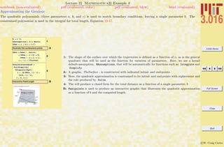
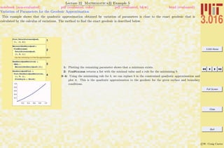
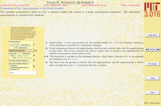
352. 3.016 Home
Full Screen
Close
Quit
c W. Craig Carter
Shortest Time Paths: The Brachiostone
The geodesic gave the shortest-distance path between two points—a related question is, “Given a velocity, what is the quickest
(shortest time) path between two points?” The answer is related the brachistochrone which is the path of most rapid descent
with constant acceleration. I don’t know what to call the shortest-time path, so I am making up a name “ brachiostone”.
Perhaps a better name would be the Fermatic, becase the curve is related to a generalized Fermat’s theorem. However, this
could be confused with fermata which is a pause of unspecified length; so I suppose that MiniFermatizoid might be the best
choice of all. However, in future editions to these notes, I am going to change the name to Brakkes’ Chrone, in honor of one
of my heros, Ken Brakke http://www.susqu.edu/brakke/. Neologisms are so entertaining—and a delightful waste of time.
For traversing a hill, it is a reasonable model for running speed to be a decreasing function of climbing-angle α, and to have
the speed fall to zero when the trajectory is “straight-up.” Thus, we select a model such as
v(s) = cos(α(s)) (22-19)
where s is the arclength along the path. The maximum speed occurs on flat ground α = 0 and running speed monotonically
falls to zero as α → π/2. To calculate the time required to traverse any path y(x) with endpoints y(0) = 0 and y(1) = 1,
ds
dt
= v(s) = cos(α(s)) =
local horizontal
local arclength
=
dx2 + dy
dx
2
dx2 + dy2 + dh2
therefore dt =
ds
v(s)
=
dx2 + dy2 + dz2
dy2 + dx2
=
1 + dy
dx
2
+ dh
dx
2
1 + dy
dx
2
dx
therefore time[y(x)] =
xe
xb
1 + dy
dx
2
+ dh
dx
2
1 + dy
dx
2
dx
(22-20)
Tthe hill h(x) = x2 can be inserted into Equation 22-20 for the time as a functional of the path between fixed points (0, 0, 0)
and (1, 1, 1).

353. 3.016 Home
Full Screen
Close
Quit
c W. Craig Carter
Lecture 22 Mathematica R Example 7
Approximating the Brachiostone by Variation of Parameters
notebook (non-evaluated) pdf (evaluated, color) pdf (evaluated, b&w) html (evaluated)
The same method for finding an approximation to the geodesic is applied to the minimum-time functional in Equation 22-20. (See
preceding text on definition of brachiostone.)
1
TotalTimeQuad =
FullSimplify@Integrate@
H1 + D@YBCs, xD^2 +
D@h, xD^2L ê
Sqrt@1 + D@YBCs, xD^2D,
8x, 0, 1<D,
Assumptions Ø b ! 1D
AVisualizing the Approximation to
the Brachiostone
4Plot@TotalTimeQuad,
8b, -2, 2<D
5
BminsolBrachioQuad =
FindMinimum@
TotalTimeQuad, 8b, 0, 1<D
6
BrachioQuadSolution =
YBCs ê.
BminsolBrachioQuad@@2DD
7
BrachioQuadPlot =
Plot@BrachioQuadSolution,
8x, 0, 1<,
PlotStyle Ø ThickD
1: The same quadratic (constrained to the boundary conditions) as was used for the geodesic is uti-
lized for the brachiostone (Equation 22-20). In this case, there is a closed-form solution for the
undetermined parameter, but this not typical for other functionals.
A: The brachiostone approximation is visualized by superposing onto the “hill” with the exact geodesic.
4: Plotting the time as a function of b indicates that there is a minimizing b.
5–7: The minimizing b is inserted back into the quadratric approximation

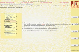
354. 3.016 Home
Full Screen
Close
Quit
c W. Craig Carter
Introduction to Calculus of Variations
Suppose the functional depends on one function of single variable, y(x), and its derivative, y (x). Furthermore, consider the
fixed end-point problem (i.e., y(xb) = yb and y(xe) = ye are specified.
The general form of the functional is:
F[y(x)] =
xe
xb
f[x, y(x), y (x)] dx (22-21)
We want to introduce a notation for functions that are “nearby” to a function y(x)15 To do this, let a function near to y(x)
be described as y(x) + v(x)∆t. (It may be useful to think of t as a time-like variable and v(x) is the instantaneous local
velocity away from y(x); but, generally, t, could be any scalar parameter.) Because y(x) is assumed to match the boundary
conditions, any admissible variation y+v∆t must also match the boundary conditions, so the ‘velocity’ v(x) at the boundaries
must vanish. Therefore, for functions near to y(x),
F[y + v∆t] =
xe
xb
f[x, y(x) + v(x)∆t, y (x) + v (x)∆t] dx (22-22)
Both sides depend on the scalar quantity ∆t, and so we will expand about ∆t = 0. We treat the integrand f(x, y, y ) as a
function of three variables (it is afterall, because f is being evaluated pointwise in the integral). Therefore, partial derivative
must appear in the expansion:
F[y] +
δF
δy ∆t=0
v∆t =
xe
xb
f[x, y(x), y (x)] dx +
xe
xb
∂f
∂y
v(x) +
∂f
∂y
v (x)
∆t=0
∆t dx (22-23)
where we use a “δ” to indicate the variational derivative of a functional. Cancelling common terms and integrating by parts,
δF
δy ∆t=0
v∆t = ∆t y(x)v(x)
xe
xb
+
xe
xb
∂f
∂y
−
d
dx
∂f
∂y ∆t=0
v(x) dx (22-24)
15
A precise definition of “closeness” of functions is somewhat arbitrary and depends on the ‘norm’ defined for functions (and because gradients
have a length and a direction, variational gradients also depend on the norm). Typically, variational calculus is introduced with the l2-norm,
f(x)·g(x) ≡
R
f(x)g(x)dx, and the resulting variation becomes δF ·v∆t =
R
[∂F/∂y −(d/dx)∂F/∂y ]v∆t which, for any h that satifies the boundary
conditions, can equal zero only if the integrand of the variation vanishes (i.e, if the variation is ‘orthogonal’ to an arbitrary h. For several applications
of other norms to materials science, see ”Variational methods for microstructural-evolution theories”, Carter W.C., Taylor J.E, Cahn J.W., JOM
(Journal of the Materials Soc.), 49(12) 30–36, 1997

355. 3.016 Home
Full Screen
Close
Quit
c W. Craig Carter
Because v(x) must vanish at the end-points, and because the terms that are being evaluated at t = 0 do not depend on t,
then
δF
δy
· v =
xe
xb
∂f
∂y
−
d
dx
∂f
∂y
v(x) dx (22-25)
Because v(x) is arbitrary (except for satisying the boundary conditions), the only way that the functional derivative can
vanish is for
∂f
∂y
−
d
dx
∂f
∂y
= 0 (22-26)
which is called the Euler equation and is the condition for a functional to be extremal with respect to a variation of its
function-argument, y(x).
We could also think of Equation 22-25 as representing the integral-sum of the instantaneous changes in the scalar value of
the functional as its function y(x) changes. The functional is stationary (i.e., a necessary condition for an extremum) if the
variational derivative vanishes everywhere on xb < x < xe. Because we have a condition as a function of a single variable, the
form of Euler’s equation in Equation 22-26 is an ordinary differential equation of derivatives of y(x) in x.
For example, consider the geodesic problem from the above example on the surface h(x) = x2, with fixed end-points y(x =
0) = 0 and y(x = 1) = 1. The functional is
F[y(x)] =
1
0
1 +
dy
dx
2
+
dh
dx
2
dx =
1
0
1 +
dy
dx
2
+ 4x2 dx (22-27)
therefore,
∂f
∂y
=0 and
∂f
∂y
=
dy
dx
1 + 4x2 + dy
dx
2
d
dx
∂f
∂y
=
d2y
dx2
1 + 4x2 + dy
dx
2
−
dy
dx 8x + 2dy
dx
d2y
dx2
1 + 4x2 + dy
dx
2 3/2
=
1 + 4x2 d2y
dx2 − 4xdy
dx
1 + 4x2 + dy
dx
2 3/2
(22-28)

356. 3.016 Home
Full Screen
Close
Quit
c W. Craig Carter
The Euler equation becomes
4xdy
dx − (1 + 4x2)d2y
dx2
(1 + 4x2 + dy
dx
2
)3/2
= 0 (22-29)
The numerator can be set equal to zero, and the result is an integrable second-order linear ODE.
This and the example for the brachiostone is demonstrated in the following examples.

357. 3.016 Home
Full Screen
Close
Quit
c W. Craig Carter
Lecture 22 Mathematica R Example 8
Euler’s equation and Exact Solution to Geodesic
notebook (non-evaluated) pdf (evaluated, color) pdf (evaluated, b&w) html (evaluated)
The variational derivative from the package VariationalMethods is used with DSolve to calculate the exact geodesic for which an
approximate solution was found above.
1Needs@
"VariationalMethods`"D
2
DistanceIntegrand = Sqrt@
H1 + HD@y@xD, xDL^2 +
HD@h, xDL^2LD
3VariationalD@
DistanceIntegrand, y@xD, xD
4
DistanceExtremalCondition =
EulerEquations@
DistanceIntegrand,
y@xD, xD
5
DistanceMinimizingFunction
= DSolve@
8DistanceExtremalConditiÖ
on, y@0D ã 0,
y@1D ã 1<, y@xD, xD
6
DistanceYExactSolution =
y@xD ê.
DistanceMinimizingFunctiÖ
on@@1DD
1: The VariationalMethods package has functions for many methods in the calculus of variations. We
will use only a few of the simpler methods in this and the following example.
2: DistanceIntegrand is the integrand for total length; it will play the role of f[x, y, y ] in Equation 22-26
3: VariationalD computes the right-hand-side of the expression in Equation 22-25.
4: EulerEquations gives the equations, for a given integrand, for the extremal solution. DistanceEx-
tremalCondition will be the ordinary differential equation, Equation 22-28.
4–5: Using DSolve to solve Euler’s equation with the boundary conditions produces the exact solution.

358. 3.016 Home
Full Screen
Close
Quit
c W. Craig Carter
Lecture 22 Mathematica R Example 9
Euler’s equation and Numerical Solution to Brachiostone
notebook (non-evaluated) pdf (evaluated, color) pdf (evaluated, b&w) html (evaluated)
The Euler’s equation for the total-time function defined in Equation 22-20 is solved by numerical methods.
This is the form of the total time's integrand as
derived above for v(s) = cos(a)
1
TimeIntegrand =
H1 + HD@y@xD, xDL^2 +
HD@h, xDL^2L ê
Sqrt@1 + HD@y@xD, xDL^2D
2
TimeExtremalCondition =
EulerEquations@
TimeIntegrand, y@xD, xD
This ODE doesn't have a closed-form solu-
tion; so we find a numerical approximation to
the solution to the Euler equation, extract it
and then plot it.
3
BrachioMinimizerNumerical =
NDSolve@
8TimeExtremalCondition,
y@0D ã 0,
y@1D ã 1<, y@xD, xD
4
BrachioNumerical = y@xD ê.
BrachioMinimizerNumerical
@@1DD
1: TimeIntegrand is the term that was derived in Equation 22-20 and used in the approximate method
for the brachiostone calculation.
2: The Euler equations for this integrand produces a non-linear second-order ODE that doesn’t have a
closed form solution.
3–4: However, a numerical solver NDSolve can be employed. In this case NDSolve runs into a few
numerical difficulties around x = 0.5, but it produces a very reasonable solution that ‘beats’ the
approximation given above.

359. 3.016 Home
Full Screen
Close
Quit
c W. Craig Carter
Lecture 22 Mathematica R Example 10
Visualizing the Brachiostone and Comparison to the Approximation Obtained by Variation of Parameters
notebook (non-evaluated) pdf (evaluated, color) pdf (evaluated, b&w) html (evaluated)
The numerical solution obtained above is plotted and compared to the approximate solution.
1
BrachioExactPlot =
Plot@BrachioNumerical,
8x, 0, 1<, PlotStyle Ø
8Thick, Darker@GreenD<D
2
GraphicsRow@
8Show@BrachioQuadPlot,
BrachioExactPlotD ,
Show@ Plot@
BrachioNumerical -
BrachioQuadSolution,
8x, 0, 1<, PlotStyle Ø
8Thickness@0.005D,
Hue@1D<DD<D
3
Time@f_D :=
Integrate@TimeIntegrand ê.
y'@xD Ø D@f, xD,
8x, 0, 1.0<D
4
N@Time@BrachioNumericalDD <
Chop@Time@
BrachioQuadSolutionDD <
Time@xD
True
1–2: This visualized the computed brachistone. It indicates that a better (and reasonable) strategy that
it is advantageous to run up-hill when the slope is small, and then traverse over a longer distance
with reduced slope (as in a “switch-back” in a hiking trail). In this case, the quadratic approximation
is still quite good, but not as good as in the geodesic.
3: This function takes a function of x for an argument and returns the total time assuming the v(s) =
cos α(s) model on a hill given by h = x2
.
4: This demonstrate that the numerical solution to the Euler equation has a shorter time than the
quadratic approximation which, in turn, is shorter than the ”projected-straight-line.” In this in-
equality, we use N with Integrate which is equivalent to using NIntegrate. The quadratic solution
has a small imaginary part that arises from numerical imprecision—this is removed with Chop.

360. 3.016 Home
Full Screen
Close
Quit
c W. Craig Carter
Harmonic Oscillators
Methods for finding general solution to the linear inhomogeneous second-order ODE
a
d2y(t)
dt2
+ b
dy(t)
dt
+ cy(t) = F(t) (22-30)
have been developed and worked out in Mathematica R examples.
Eq. 22-30 arises frequently in physical models, among the most common are:
Electrical circuits: L
d2I(t)
dt2
+ ρlo
dI(t)
dt
+
1
C
I(t) = V (t)
Mechanical oscillators: M
d2y(t)
dt2
+ ηlo
dy(t)
dt
+ Ksy(t) = Fapp(t)
(22-31)
where:
Mechanical Electrical
Second
Order
Mass M: Physical measure of the ratio
of momentum field to velocity
Inductance L: Physical measure of the
ratio of stored magnetic field to current
First
Order
Drag Coefficient c = ηlo
(η is viscosity lo is a unit displacement):
Physical measure of the ratio environ-
mental resisting forces to velocity—or
proportionality constant for energy
dissipation with square of velocity
Resistance R = ρlo
(ρ is resistance per unit material length
lo is a unit length): Physical measure of
the ratio of voltage drop to current—or
proportionality constant for power dissi-
pated with square of the current.
Zeroth
Order
Spring Constant Ks: Physical measure
of the ratio environmental force developed
to displacement—or proportionality con-
stant for energy stored with square of dis-
placement
Inverse Capacitance 1/C: Physical
measure of the ratio of voltage storage
rate to current—or proportionality con-
stant for energy storage rate dissipated
with square of the current.
Forcing
Term
Applied Voltage V (t): Voltage applied
to circuit as a function of time.
Applied Force F(t): Force applied to
oscillator as a function of time.

361. 3.016 Home
Full Screen
Close
Quit
c W. Craig Carter
For the homogeneous equations (i.e. no applied forces or voltages) the solutions for physically allowable values of the coefficients
can either be oscillatory, oscillatory with damped amplitudes, or, completely damped with no oscillations. (See Figure 21-21).
The homogeneous equations are sometimes called autonomous equations—or autonomous systems.
Simple Undamped Harmonic Oscillator
The simplest version of a homogeneous Eq. 22-30 with no damping coefficient (b = 0, R = 0, or η = 0) appears in a remarkably
wide variety of physical models. This simplest physical model is a simple harmonic oscillator—composed of a mass accelerating
with a linear spring restoring force:
Inertial Force = Restoring Force
MAcceleration = Spring Force
M
d2y(t)
dt2
= −Ksy(t)
M
d2y(t)
dt2
+ Ksy(t) = 0
(22-32)
Here y is the displacement from the equilibrium position–i.e., the position where the force, F = −dU/dx = 0. Eq. 22-32 has
solutions that oscillate in time with frequency ω:
y(t) = A cos ωt + B sin ωt
y(t) = C sin(ωt + φ)
(22-33)
where ω = Ks/M is the natural frequency of oscillation, A and B are integration constants written as amplitudes; or, C
and φ are integration constants written as an amplitude and a phase shift.

362. 3.016 Home
Full Screen
Close
Quit
c W. Craig Carter
The simple harmonic oscillator has an invariant, for the case of mass-spring system the invariant is the total energy:
Kinetic Energy + Potential Energy =
M
2
v2
+
Ks
2
y2
=
M
2
dy
dt
2
+
Ks
2
y2
=
A2
ω2 M
2
cos2
(ωt + φ) + A2 Ks
2
sin2
(ωt + φ) =
A2
(ω2 M
2
cos2
(ωt + φ) +
Mω2
2
sin2
(ωt + φ) =
A2
Mω2
= constant
(22-34)
There are a remarkable number of physical systems that can be reduced to a simple harmonic oscillator (i.e., the model can
be reduced to Eq. 22-32). Each such system has an analog to a mass, to a spring constant, and thus to a natural frequency.
Furthermore, every such system will have an invariant that is an analog to the total energy—an in many cases the invariant
will, in fact, be the total energy.
The advantage of reducing a physical model to a harmonic oscillator is that all of the physics follows from the simple harmonic
oscillator.
Here are a few examples of systems that can be reduced to simple harmonic oscillators:
Pendulum By equating the rate of change of angular momentum equal to the torque, the equation for pendulum motion
can be derived:
MR2 d2θ
dt2
+ MgR sin θ = 0 (22-35)
for small-amplitude pendulum oscillations, sin(θ) ≈ θ, the equation is the same as a simple harmonic oscillator.
It is instructive to consider the invariant for the non-linear equation. Because
d2θ
dt2
=
dθ
dt
ddθ
dt
dθ
(22-36)

363. 3.016 Home
Full Screen
Close
Quit
c W. Craig Carter
Eq. 22-35 can be written as:
MR2 dθ
dt
ddθ
dt
dθ
+ MgR sin(θ) = 0 (22-37)
d
dθ
MR2
2
dθ
dt
2
− MgR cos(θ) = 0 (22-38)
which can be integrated with respect to θ:
MR2
2
dθ
dt
2
− MgR cos(θ) = constant (22-39)
This equation will be used as a level-set equation to visualize pendulum motion.
Buoyant Object Consider a buoyant object that is slightly displaced from its equilibrium floating position. The force
(downwards) due to gravity of the buoy is ρbouygVbouy The force (upwards) according to Archimedes is ρwatergVsub where
Vsub is the volume of the buoy that is submerged. The equilibrium position must satisfy Vsub−eq/Vbouy = ρbouy/ρwater.
If the buoy is slightly perturbed at equilibrium by an amount δx the force is:
F =ρwaterg(Vsub−eq + δxAo) − ρbuoygVbuoy
F =ρwatergδxAo
(22-40)
where Ao is the cross-sectional area at the equilibrium position. Newton’s equation of motion for the buoy is:
Mbuoy
d2y
dt2
− ρwatergAoy = 0 (22-41)
so the characteristic frequency of the buoy is ω = ρwatergAo/Mbouy.
Single Electron Wave-function The one-dimensional Schr¨odinger equation is:
d2ψ
dx2
+
2m
2
(E − U(x)) ψ = 0 (22-42)
where U(x) is the potential energy at a position x. If U(x) is constant as in a free electron in a box, then the one-
dimensional wave equation reduces to a simple harmonic oscillator.
In summation, just about any system that oscillates about an equilibrium state can be reduced to a harmonic oscillator.

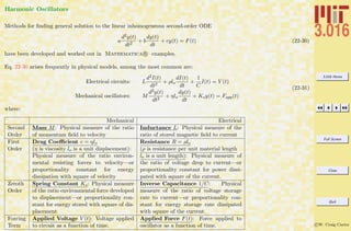
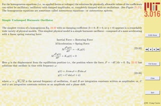
364. 3.016 Home
Full Screen
Close
Quit
c W. Craig Carter
Index
:= delayed evaluation, 46
→
rules, 35
.
Mathematica’s matrix multiplication, 85
., 92
/.
replacement, 35
/., 44, 325
//., 325
/;, 44, 325
:->, 44
:=, 45, 225
:>, 325
;, 39
<<, 57, 58
=, 31, 45, 225
==, 31
>>, 57
[], 32
$Assumptions, 331
$RecursionLimit, 47
Assumptions
use in Simplify, 51
Integrate
using Assumptions, 52
Simplify
using Assumptions, 51
Simplify doesn’t simplify
√
x2?, 51
{}, 34
Abs, 107, 256
AbsoluteOptions, 73, 74
academic honesty
MIT policy, 7
AFunction, 235
All, 34
Ampere’s law, 229
amplitude vectors, 242
angle, 206
Animate, 72, 73
animation
example projection into three dimensions, 209
of random walk, 73
animation example
a vector and its trajectory, 144
animations
if each frame is expensive to compute, 194
of time-dependent phenomena, 71
anisotropic surface energy
example of integrating over surface, 213
Annotation, 65
annotation
example
in three-dimensional graphics, 103
Apart, 51
Append, 304
AppendTo, 75

365. 3.016 Home
Full Screen
Close
Quit
c W. Craig Carter
Approxfunction, 165
ApproxPlot, 165
ArcCos, 31
arclength, 155
as a parameter, 156
area vector, 127
Arg, 107
arguments with default values, 77
array of charges
visualization example, 67
ArrayPlot, 254, 256
AScalarFunction, 161
assigned reading, 10
Assuming, 239
Assumptions, 51, 149, 219
assumptions
simplifying roots, 51
asymptotic behavior, 281
AtomDensityWithDefect, 261
autonomous systems, 343
avian, 232
AvocadoColors, 226
axes, 104
AxesLabel, 33, 60
axis labels, 33
bagpipe, 232
BarChart, 66
BarCharts, 66
BarLabels, 66
BarOrientation, 66
BaseStyle, 33, 60
BasicMathInput, 60
basis, 123
basis functions, 243
basis vectors, 100
eigenvalue representations, 137
beam boundary conditions
clamped, 317
free, 316
point load, 317
beam deflections, 318
beam equation, 315
BeamEquation, 318
BeamViz, 319
Beethoven, 232
Bendy, 157
Bernoulli equation, 298
BernoulliEquation, 299
Boomerang, 235
Boston
distance to Paris, 178
BotContribution, 223
boundary conditions
Dirichlet and Neumann, 313
boundary values
in second order ODEs, 313
boxload, 318, 319
brachiostone, 334
brachistochrone, 334
Brakke, Ken
The Surface Evolver, 180
Brakkes’ Chrone, 334

366. 3.016 Home
Full Screen
Close
Quit
c W. Craig Carter
C[1], 297
C[1],C[2],etc, 284
C[N], 296
calculus of many variables, 160
Calendar, 58
calendar
course, 11
homework, 9
Cartesian, 186
CartesianCoordinatesofCity, 178
Cases, 44, 66
chain rule
for several variables, 161
change of variables
in first-order non-linear ODE, 299
ChangeofChangeper∆, 303
Changeper∆, 303
changing variables
jacobian, 190
characteristic length, time for diffusion equation, 149
ChemicalElements, 64
Chop, 98, 110, 341
CircAps, 263
Circle, 69, 235
CityData, 178
Clamp, 318
Clear, 27, 28
codimension, 153
Coefficient, 51, 143
coefficient matrix
form in Mathematica, 92
Collect, 33, 51, 131
ColOct, 102
ColorData, 67, 68, 150
ColorFunction, 63, 67, 68, 150, 173, 206, 207, 255, 256
ColorFunctionScaling, 68, 72, 194
columns of a matrix, 85
common errors in Mathematica, 26
common tangent construction
visualization of, 74
CommonTangentConstruction, 77, 78
commutation
physical interpretation, 99
commute, 99
commuting matrices
physical interpretation, 99
Complex, 48
complex conjugate, 108
complex numbers
opearations on
polar representation, 109
operations on, 107
polar representation, 109
raising to a power, 111
geometrical interpretation, 111
relations to trignometric functions, 111
spanning vectors for, 105
complex plane, 108
complex roots to polynomial equations
examples, 112
complex values
in plots, 112
ComplexExpand, 107, 112
compliance tensor, 91

367. 3.016 Home
Full Screen
Close
Quit
c W. Craig Carter
computation speed
using memory to increase, 47
computational efficiency
linear systems of equations, 93
ComputationalGeometry, 75
Condition, 44, 325
condition pattern matching, 48
conditional definition (/;), 49
conditions
finding parameters subject to constraint, 311
conjugation
as a reflection in the complex plane, 108
conservative, irrotational, curl free fields, 182
ConstantRule, 325
ConstFunction, 211
constraints
determining parametric conditions, 311
ContourPlot, 68, 149, 173, 194, 200, 225, 226
ContourPlot3D, 211
Contours, 68, 194, 211
ContrastGraphics, 255
convex hull, 75
ConvexHull, 75
convolution of two functions, 252
convolution theorem, 252
physical interpretation, 253
coordinate systems
gradients and divergence computations, 179
Coordinate Transformations, 177
coordinate transformations, 177
CoordinatesFromCartesian, 177
CoordinatesToCartesian, 177
corners, 104
course calendar, 11
cplot, 194
cplots, 194
CrazyFun, 165
Cross, 143
cross product, 143
geometric interpretation, 142
CrossProduct, 213
crystal point group, 104
crystal structures
relative fractions among elements, 66
Curl, 186
curl
interpretations, 180
curl free, irrotational, conservative fields, 182
curl of a vector functions and path independence, 185
CurlOfOneStooge, 188
current directory, 57
curvature
formula in terms of arclength, 155
grain boundary, 289
curvature vector, 155
CurvatureOfGraph, 206
curve
local orthonormal frame, 156
curves and surfaces, 152
displaying together
example, 154
curves in space
examples of, 144, 146
Cylinder, 144

368. 3.016 Home
Full Screen
Close
Quit
c W. Craig Carter
CylinderContribution, 221
CylinderIntegrandθζ, 220
CylinderIntegranddθ, 221
CylinderIntegrandUpperZdθ, 221
cylindrical coordinate system
vectors in, 79
cylindrical coordinates, 177
form of gradient and divergence, 179
D, 33, 40, 52, 146, 277
DampedHOAssumptions, 327
damping factors, 343
Darker, 301
data
using mouse-over to annotate, 65
data visualization, 64
DateList, 58
DayOfWeek, 58
Degree, 178
delayed assignment, 45
delayed assignment :=, 26
delayed evaluation :=, 46
delayed evaluation :=
when not to use in function definitions, 225
delayed ruleset, 44
DeleteCases, 66
delta functions, 251
DeMoivre’s formula, 109
density conservation
Parseval’s theorem, 252
density fields of extensive quantities, 158
density—melting point
histogram for elements, 66
derivatives
example, 52
derivatives of integrals, 189
derivatives of scalar functions, 158
Det, 87, 92, 95, 143
determinant, 87
determinants, 92
properties of, 96
diagonalize a matrix, 123
difference relation, 303
DifferenceRelation, 303
differential equations, 268
differential forms in thermodynamics, 292
differential operators, 321
Diffraction
simulated, 259
three-dimensional representations of two-dimensional data,
260
diffraction, 249
interactive simulation of lattice diffraction, 266
simulated, 258
DiffractionMicroscopy, 263, 265–267
diffusion equation
example of visualizing, 72
example planar solution rectangular initial conditions, 149
dimensional scaling, 72
dimensionless forms
example of creating, 219
Dimensions, 34, 85, 112
Dirac delta function
Fourier transforms, 324

369. 3.016 Home
Full Screen
Close
Quit
c W. Craig Carter
Dirac delta functions, 251
Dirac-delta function
as point load on beam, 315
DiracDelta, 320
Directive, 154, 211
Directory, 57
Dirichlet boundary conditions, 313
discrete Fourier transforms with Mathematica, 258
DisplayForm, 34
DistanceExtremalCondition, 339
DistanceIntegrand, 339
Distribute, 325
DistributeRule, 325
Div, 219
divergence
example calculation and visualization, 175
interpretations, 174
divergence, 175
divergence theorem, 215
example of Hamaker interaction, 219
example of London Dispersion Interaction, 219
relation to accumulation at a point, 216
Divisors, 42
Do, 39
Drawing Tools Widget, 69
Drop, 75
DSolve, 284, 285, 287, 296, 297, 299, 300, 318, 320, 327, 339
Dynamic, 135, 194
dynamic graphics
enclosed within Manipulate, 135
DynamicModule, 135
efficiency
storing intermediate iteration values, 270
eigenbasis, 137
transformations to, 123
eigenframe representation of surface patch, 201
eigenfunction, 322
Eigensystem, 115
eigensystems
example of four spring-connected masses, 118
harmonic oscillator, 116
lattice vibrations, 117
one-dimensional Shr¨odinger wave equation, 119
stress and strain, 130
eigenvalue
of an operator, 322
EigenValues, 28
Eigenvalues, 28, 115
Eigenvectors, 115
eigenvectors, eigenvalues, and eigensystems for matrix equa-
tions, 113
Einstein summation convention, 90
elastic energy density, 91
electrical circuits as harmonic oscillators, 342
electrostatic potential
above a triangular patch of constant charge density, 194
element properties
visualization, 64
ElementData, 64
Eliminate, 89
embedded curve, 160
embedded curves in surfaces
visualization example, 154

370. 3.016 Home
Full Screen
Close
Quit
c W. Craig Carter
embedded surface, 160
embedding space, 152
energy dissipations and quadratic forms, 136
entropy
ideal entropy of mixing, 49
Euler equation, 337
Euler integration, 273
EulerEquations, 339
Evaluate
using in function definitions, 179
Evaluate, 28, 62, 112, 179, 206, 221, 224, 225, 277, 301
even and odd functions, 236
EvenAmplitudeVector, 243
EvenAmplitudeVectors, 242
EvenBasisVector, 243
EvenTerms, 242
Evolve, 271
Example function
AFunction, 235
AScalarFunction, 161
ApproxPlot, 165
Approxfunction, 165
AtomDensityWithDefect, 261
BeamEquation, 318
BeamViz, 319
Bendy, 157
BernoulliEquation, 299
Boomerang, 235
BotContribution, 223
CartesianCoordinatesofCity, 178
ChangeofChangeper∆, 303
Changeper∆, 303
CircAps, 263
Clamp, 318
ColOct, 102
CommonTangentConstruction, 77, 78
ConstFunction, 211
ConstantRule, 325
ContrastGraphics, 255
CrazyFun, 165
CurlOfOneStooge, 188
CurvatureOfGraph, 206
CylinderContribution, 221
CylinderIntegrandθζ, 220
CylinderIntegrandUpperZdθ, 221
CylinderIntegranddθ, 221
DampedHOAssumptions, 327
DifferenceRelation, 303
DiffractionMicroscopy, 263, 265–267
DistanceExtremalCondition, 339
DistanceIntegrand, 339
DistributeRule, 325
EvenAmplitudeVectors, 242
EvenAmplitudeVector, 243
EvenBasisVector, 243
EvenTerms, 242
Evolve, 271
ExplFun, 271
ExpleFun, 270
FCC, 104
FPlot, 243
FlowerPot, 154
FourierRowK0, 259
FourierRow, 258, 259

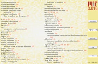
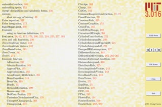
371. 3.016 Home
Full Screen
Close
Quit
c W. Craig Carter
FreeBeam, 318
FuncEx, 274, 284
GenlSol, 314
GeodesicExact, 333
Gmolar, 75
GrainStructure, 264
GraphFunction, 206
GrowList, 304, 305
ImagePlot, 256
KZeroAtCenter, 259
KZeroMiddle, 259
Knob, 318
LatLong, 178
LeavingKansas, 181
MagicCircles[t,n], 63
ManipulateTruncatedFourierSeries, 245
NoisyLattice, 262
NormalizeRules, 72
Note, 231
OddAmplitudeVector, 242, 243
OddBasisVector, 243
OddTerms, 242
OrbitOrbit[r,t,n], 63
PVecLondon, 219
PathDepInt, 186
Pform, 107
PlotM1, 275
PlotTrajs, 272
PrettyFlower, 157
PushMethod1, 274, 275
PushMethod2, 277
RanRest, 233
RandMat, 98
RandomInstruments, 233
RandomNotesandRests, 233
RandomNotes, 233
ReduceHalfHalf, 244
ReducedFunction, 244, 246
ScaleRules, 149, 219
SheetOLatticeCharge, 67
SimplePot, 179
SomeNoise, 262
SphericalCoordinatesofCity, 178
Spots3DRow, 260
Spots3D, 260
Stooge, 188
SurfaceParametric, 210
SurfaceTension, 213
TheODE, 310
TheSurface, 331
ThreeHolePotential, 173, 175
TimeIntegrand, 340
TopContribution, 222
ToutesDesLoups, 70
Traj, 271, 272
TrianglePotentialNumeric, 194
UnitNormal, 213
VanishOnCylinder, 188
VectorFunction, 186
Vines, 154
XLogX, 49
XVector, 144
angle, 206
avian, 232

372. 3.016 Home
Full Screen
Close
Quit
c W. Craig Carter
axes, 104
bagpipe, 232
boxload, 318, 319
corners, 104
cplots, 194
cplot, 194
divergence, 175
faces, 104
factorial, 48
fccmodel, 104
fccsites, 104
gline, 73
gradfield, 173, 175
gtext, 73
highcontrast, 255, 260
identity, 103
linearload, 318
midload, 318
modcircledemo, 235
modmatdemo, 235
mohrs, 134
ncplot, 200
noload, 318
normalcontrast, 255
notes, 231, 232
note, 231
octa, 102
pface, 209
piano, 232
potential, 173
purenote, 231, 232
randomwalk, 73
ref[010], 103
rot90[001], 103
scaledconc, 149
simtrans, 123
srad, 104
transoct, 103
unitload, 318
vp, 208
wulffline, 70
xlogx, 74
Exclusions, 62, 226
executing command with shift-enter
difference between entering text, 29
Expand, 32, 33, 51, 164
ExpleFun, 270
ExplFun, 271
exponential growth and decay, 270
expressions to functions
converting, 224
extensive quantities
density fields, 158
extent of chemical reaction, 151
extremal functions, 328
faces, 104
Factor, 33, 51, 87
factorial, 48
factorial function
examples of defining, 47
fast Fourier transforms, 258
fast fourier transforms, 257
FCC, 104

373. 3.016 Home
Full Screen
Close
Quit
c W. Craig Carter
FCC crystal
visualization of, 104
fccmodel, 104
fccsites, 104
fermata, 334
Fermatic, 334
Fick’s first law, 148, 150
Fick’s second law, 216
fields of intensive quantities, 158
FilePrint, 57
filestream, 57
Filling, 62
filling
between curves, 62
FindInstance, 186
FindMinimum, 40, 332
FindRoot, 40, 55
finite differences, 274
implicit methods, 277
first-order explicit finite differencing, 273
first-order finite difference operator, 303
first-order ordinary differential equations
geometry, 279
Flatten, 104, 284
FlowerPot, 154
flux, 148
visualization of, 150
visualization of flux through surface, 215
For, 39, 40
force
relations to stress, 127
forces
in harmonic oscillator model, 343
Fourier series, 237
complex form, 247, 249
example functions for computing, 242
example of convergence of truncated, 243
mapping the periodic domain to (-1/2,1/2)., 244
plausibility of infinite sum, 237
the orthogonality trick, 238
Fourier transform
as a linear operator, 323
as a method to solve ODEs, 323
as limit of infinite domain Fourier series, 250
Fourier transforms, 248
higher dimensional, 250
Fourier transforms on graphical images, 267
FourierCosCoefficient, 244
FourierRow, 258, 259
FourierRowK0, 259
FourierSeries, 244
FourierSinCoefficient, 244
FourierTransform, 325, 326
FourierTrigSeries, 244
FPlot, 243
FreeBeam, 318
FreeQ, 325
Frenet equations, 156
freq, 231
frequency
harmonic oscillator, 343
FrontEnd, 29, 30
FullSimplify, 33, 206, 219, 327
FuncEx, 274, 284

374. 3.016 Home
Full Screen
Close
Quit
c W. Craig Carter
Function, 206
function basis, 307
function decomposition into odd and even parts, 236
function definitions
restrictions on the arguments, 48
function definitions in Mathematica
when to use = or :=, 224
functionals, 328
functions
creating in Mathematica, 43
defining with patterns, 45
sound of, 231
storing intermediate values, 270
functions from expressions, 224
functions in programming, 37
functions of functions, 328
functions that remember previously calculated values., 47
fundamental theorem of calculus
generalizations to higher dimensions, 214
relation to divergence and Stokes’ theorem, 214
fundamental theorem of differential and integral calculus, 196
Gauss’ law, 229
GenlSol, 314
geodesic, 328
GeodesicExact, 333
Geodesy, 178
GeometricTransformation, 104
Gibbs phenomenon, 246
gline, 73
Glow, 102, 207
Gmolar, 75
Grad, 179
grad, div, and curl, 171
gradfield, 173, 175
gradient field, 148
gradient fields
visualization of, 150
gradient of scalar function
path independence, 185
gradients, 161, 168
example calculation and visualization, 173
grading policy, 5, 8
grain boundary, 265
grain boundary energy, 289
grain boundary mobility, 290
grain growth, 288
grains
simulation for diffraction, 264
GrainStructure, 264
Gram-Schmidt, 123
GramSchmidt, 123
graph surfaces
visualization example, 206
GraphFunction, 206
graphical primitives, 134
Graphics, 69, 235
graphics
building up descriptive graphics step-by-step, 311
graphical interaction
simple example, 61
graphics primitives, 69
mesh control, 61
reflection from default light sources, 102

375. 3.016 Home
Full Screen
Close
Quit
c W. Craig Carter
graphics in mathematica
examples, 59
Graphics Object, 69
Graphics Primitives, 69
Graphics3D, 102, 103, 208, 209, 280
GraphicsColumn, 235
GraphicsGrid, 103, 207
GraphicsRow, 301
Green’s function, 149
Green’s theorem in the plane
relation to Stoke’s theorem, 197
turning integrals over simple closed regions to their bound-
aries, 195
visual interpretation, 196
visualization, 214
GreenBrownTerrain, 68
GrowList, 304, 305
gtext, 73
Hamaker Interaction between cylinder and point, 226
harmonic oscillator
buoys, 345
damped forced ODE, 323
force interpretion, 326
Fourier transform of, 326
pendulum, 344
single electron wave function, 345
solutions using Fourier transforms, 323
harmonic oscillators, 342
instances in different physical phenomena, 342
harmonics, 248
heat capacity at constant volume
example of changing variables, 191
heat flux and temperature gradients, 169
help browser, 36
hermits and skew-hermits, 121
heterogeneous linear first-order ODE, 294
highcontrast, 255, 260
Histogram3D, 28, 66
Histograms, 28, 66
homework calendar, 9
homogeneous linear first-order ODE, 294
homogeneous second order ordinary differential equations, 302
homogeneous second-order linear ODE
constant coefficients, 308
Hue, 62, 68, 102, 112, 206
hydrostatic stress, 128
hyper-surface, 153
ideal entropy of mixing, 49
identity, 103
identity matrix, 86
If, 42
Im, 107, 112, 301
image depth, 71
ImagePlot, 256
ImageSize, 33, 65, 256
importing data, 56
increment structure, 39
Initialization, 246
input and output, 56
input/output, 56
Integer, 44, 48
integrals

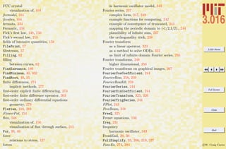
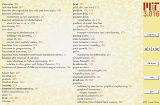
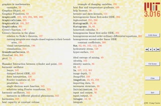
376. 3.016 Home
Full Screen
Close
Quit
c W. Craig Carter
example, 52
Integrate, 33, 52, 55, 193, 199, 239, 331
integrating factors, 292
use in thermodynamics, 293
integration
over surface, 212
integration along a path, 184
integration along curve
using arclength, 156
integration constants
form in Mathematica, 284
form of in Mathematica, 296
integration over irregularly shaped domain
example, 193
intensive fields
chemical potential, 158
pressure, 158
temperature, 158
intermediate output, 39
InterpolatingFunction, 300, 301
InterpolationFunction, 301
InterpolationOrder, 208
intial iteration value, 39
invariant
in harmonic oscillator, 344
Inverse, 87, 93
inverse Fourier transform, 324
InverseFourierTransform, 327
inversion functions
Mathematica warning, 300
inverting parametric form of curve, 156
irrotational, curl free, conservative fields, 182
isobars and the weather, 169
jacobian, 190
Join, 104
K[N], 296
Ken Brakke, 334
kernel, 30
killing vectors, 95
kinetic coefficient, 279
Knob, 318
KZeroAtCenter, 259
KZeroMiddle, 259
l2-norm, 336
lab reports
format, 4
LabelStyle, 65
LakeColors, 226
Laplacian
example calculation and visualization, 175
late policy, 9
LatLong, 178
lattice images
simulated, 254
lattice vibrations
diffraction from, 262
LeavingKansas, 181
lecture notes
use of, 10
Length, 34, 85
length minimizing path
geodesic, 328

377. 3.016 Home
Full Screen
Close
Quit
c W. Craig Carter
level set surfaces
visualization example, 211
LIFI-FILI, 193
light sources, 102
Lighting, 102, 207
Limit, 49, 52, 239
limits
example, 52
line integration, 156
linear equations
adding homogeneous solutions to the nonhomogeneous so-
lutions, 94
existence of solutions, 90
linear first-order ODEs
integral form of solution, 298
linear independence, 88
linear operators
defining rules for, 325
linear ordinary differential equations, 293
linear superposition of basis functions, 307
linear system of equations, 90
linear systems of equations
computational efficiency, 93
linear transformation of vectors, 82
linear transformations, 101
defining rules for, 325
visualization examples, 102
linear vector spaces, 100
linearization, 166
linearload, 318
LinearSolve, 93, 95
liner differential equations
superposition of solutions, 306
List, 34, 48
ListAnimate, 72, 149, 194, 209, 210
ListInterpolation, 209
ListLinePlot, 64, 65
ListPlot, 40, 64, 65, 271, 272, 275, 305
ListPlot3D, 208, 260
local orthonormal frame on curve, 156
localized variables, 42, 304
LocatorPane, 135
Log, 39, 40
logical equalities, 92
logical equality, 27
loops in programming, 37
magic integral theorems, 195
MagicCircles[t,n], 63
magnetic fields
magnetization and, 229
Manipulate
economy of, 263
Manipulate, 61, 63, 70, 78, 103, 135, 144, 146, 211, 245, 246,
263, 271, 320, 331
ManipulateTruncatedFourierSeries, 245
Markov chains, 270
materials science and mathematics, 2
Mathematica
availability, 3
common mistakes, 26
getting information, 36
help browser, 36
Mathematica function

378. 3.016 Home
Full Screen
Close
Quit
c W. Craig Carter
., 92
/., 44, 325
//., 325
/;, 44, 325
:-¿, 44
:=, 45, 225
:¿, 325
;, 39
¡¡, 57, 58
==, 31
=, 31, 45, 225
¿¿, 57
AbsoluteOptions, 73, 74
Abs, 107, 256
All, 34
Animate, 72, 73
Annotation, 65
Apart, 51
AppendTo, 75
Append, 304
ArcCos, 31
Arg, 107
ArrayPlot, 254, 256
Assuming, 239
Assumptions, 51, 149, 219
AvocadoColors, 226
AxesLabel, 33, 60
BarChart, 66
BarLabels, 66
BarOrientation, 66
BaseStyle, 33, 60
BasicMathInput, 60
C[1],C[2],etc, 284
C[1], 297
C[N], 296
Cartesian, 186
Cases, 44, 66
Chop, 98, 110, 341
Circle, 69, 235
CityData, 178
Clear, 27, 28
Coefficient, 51, 143
Collect, 33, 51, 131
ColorData, 67, 68, 150
ColorFunctionScaling, 68, 72, 194
ColorFunction, 63, 67, 68, 150, 173, 206, 207, 255, 256
ComplexExpand, 107, 112
Complex, 48
Condition, 44, 325
ContourPlot3D, 211
ContourPlot, 68, 149, 173, 194, 200, 225, 226
Contours, 68, 194, 211
ConvexHull, 75
CoordinatesFromCartesian, 177
CoordinatesToCartesian, 177
CrossProduct, 213
Cross, 143
Curl, 186
Cylinder, 144
DSolve, 284, 285, 287, 296, 297, 299, 300, 318, 320, 327,
339
Darker, 301
DateList, 58
DayOfWeek, 58

379. 3.016 Home
Full Screen
Close
Quit
c W. Craig Carter
Degree, 178
DeleteCases, 66
Det, 87, 92, 95, 143
Dimensions, 34, 85, 112
DiracDelta, 320
Directive, 154, 211
Directory, 57
DisplayForm, 34
Distribute, 325
Divisors, 42
Div, 219
Do, 39
Drop, 75
DynamicModule, 135
Dynamic, 135, 194
D, 33, 40, 52, 146, 277
EigenValues, 28
Eigensystem, 115
Eigenvalues, 28, 115
Eigenvectors, 115
ElementData, 64
Eliminate, 89
EulerEquations, 339
Evaluate, 28, 62, 112, 179, 206, 221, 224, 225, 277, 301
Exclusions, 62, 226
Expand, 32, 33, 51, 164
Factor, 33, 51, 87
FilePrint, 57
Filling, 62
FindInstance, 186
FindMinimum, 40, 332
FindRoot, 40, 55
Flatten, 104, 284
For, 39, 40
FourierCosCoefficient, 244
FourierSinCoefficient, 244
FourierTransform, 325, 326
FourierTrigSeries, 244
FreeQ, 325
FullSimplify, 33, 206, 219, 327
Function, 206
GeometricTransformation, 104
Glow, 102, 207
Grad, 179
GramSchmidt, 123
Graphics3D, 102, 103, 208, 209, 280
GraphicsColumn, 235
GraphicsGrid, 103, 207
GraphicsRow, 301
Graphics, 69, 235
GreenBrownTerrain, 68
Histogram3D, 28, 66
Hue, 62, 68, 102, 112, 206
If, 42
ImageSize, 33, 65, 256
Im, 107, 112, 301
Initialization, 246
Integer, 44, 48
Integrate, 33, 52, 55, 193, 199, 239, 331
InterpolatingFunction, 300, 301
InterpolationFunction, 301
InterpolationOrder, 208
InverseFourierTransform, 327
Inverse, 87, 93

380. 3.016 Home
Full Screen
Close
Quit
c W. Craig Carter
Join, 104
K[N], 296
LabelStyle, 65
LakeColors, 226
Length, 34, 85
Lighting, 102, 207
Limit, 49, 52, 239
LinearSolve, 93, 95
ListAnimate, 72, 149, 194, 209, 210
ListInterpolation, 209
ListLinePlot, 64, 65
ListPlot3D, 208, 260
ListPlot, 40, 64, 65, 271, 272, 275, 305
List, 34, 48
LocatorPane, 135
Log, 39, 40
Manipulate, 61, 63, 70, 78, 103, 135, 144, 146, 211, 245,
246, 263, 271, 320, 331
MatrixForm, 28, 34, 57, 85
MatrixRank, 89, 95
MatrixTransform, 123
MaxRecursion, 61
Max, 208
MemberQ, 325
MeshFunctions, 149, 206, 227
MeshStyle, 61
Mesh, 61
Min, 208
Missing, 64
Module, 42, 70, 135, 304
Mod, 235
NDSolve, 301, 340
NIntegrate, 55, 194, 200, 221
NSolve, 55
Needs, 58
NestListWhile, 274, 275
NestList, 274
NestWhile, 304, 305
Nest, 40, 274, 277
NonNegative, 48
Normalize, 123
Normal, 52, 164, 165
Norm, 178, 213
Notebook, 27
NullSpace, 89
NumberQ, 34, 48
Numerator, 51
Octahedron, 102
Opacity, 104, 154, 211
Options, 33
O, 52, 164
PLotLabel, 33
ParameticPlot3D, 146
ParametricPlot3D, 144, 154, 210
ParametricPlot, 63, 132
Part, 34
Permutations, 34, 99
PieChart, 66
Piecewise, 320
Pi, 107
Play, 231
Plot3D, 67, 72, 149, 173, 206, 207, 209, 227
PlotJoined, 64
PlotLabel, 256

381. 3.016 Home
Full Screen
Close
Quit
c W. Craig Carter
PlotMarkers, 64
PlotPoints, 61, 67, 68
PlotRange, 33, 60, 63, 73, 144, 208, 227
PlotStyle-¿Thick, 49
PlotStyle, 60, 62, 63, 112, 301
PlotVectorField, 150, 175
Plot, 28, 33, 49, 55, 60–62, 69, 72, 235, 301
Polygons, 102
Polygon, 103
PolyhedronData, 102
PopupWindow, 65
Positive, 48
PossibleZeroQ, 49
PowerExpand, 299
PrependTo, 75
PrimeQ, 42
Prime, 42
Print, 39, 42
ProgressIndicator, 194, 200
Quotient, 259
RandomReal, 57, 73
Rational, 48
Real, 48
Reduce, 311
RegionFunction, 67, 226, 227
RegionPlot, 74, 311
ReplaceAll, 44, 325
ReplaceRepeated, 325
Replace, 35
Re, 107, 112, 301
Riffle, 232
RotateRight, 259
Rotate, 104
RotationTransform, 103
Round, 110
RuleDelayed, 325
Save, 57
ScaleFactor, 150
Select, 34
SeriesData, 52
Series, 52, 164, 165
SetDirectory, 57
Short, 112
Show, 69, 70, 73, 102, 150, 226, 227, 311
Sign, 49
Simplify, 32, 33, 51–53, 87, 107, 299, 331
Solution, 53
Solve, 53, 89, 92, 95, 115, 284, 299, 310, 314, 320, 327,
331
Sort, 34, 75
SoundNote, 232
Sound, 231
Specularity, 154
Sphere, 104
SphericalDistance, 178
SphericalPlot3D, 213
SpheroidalDistance, 178
Split, 75
StatusArea, 65
StringQ, 48
Sum, 44, 53
Symbol, 48
Table, 34, 39, 62, 64, 70, 72, 75, 103, 194, 208–210, 233,
254

382. 3.016 Home
Full Screen
Close
Quit
c W. Craig Carter
Tally, 66
TextStyle, 33
Text, 103
Thickness, 62, 112
Thread, 231, 232
TickStyle, 60
Timing, 47, 194, 200
Together, 51
Tooltip, 65
Translate, 104, 146
Transpose, 34, 66, 85, 123
TrigReduce, 131
VariationalD, 339
VectorFieldPlot3D, 181
VectorFieldPlot, 281, 282
ViewPoint, 103
While, 39
[], 32
$Assumptions, 331
$RecursionLimit, 47
{}, 34
freq, 231
purenote, 231
solution, 301
Mathematica package
BarCharts, 66
Calendar, 58
ChemicalElements, 64
ComputationalGeometry, 75
FourierSeries, 244
Geodesy, 178
Histograms, 28, 66
PieCharts, 66
PolyhedronOperations, 102
VariationalMethods, 339
VectorAnalysis, 177–179, 186, 213, 219
VectorFieldPlots, 150, 175, 181, 281
Mathematica Packages, 28
mathematica packages
example, 58
Mathematica warning
inverse functions, 300
mathematical constant, 107
matrices, 81
as a linear transformation operation, 82
all eigenvalues with unit magnitude, 120
all imaginary eigenvalues, 119
all real eigenvalues, 119
column and row spaces, 81
multiplication, 84
similarity transformations, 124
special, 119
Hermitian, 119
Orthonormal, 120
Skew-Hermitian, 119
Unitary, 120
summation convention, 82
transpose combined with matrix multiplication, 83
transpose operation on, 83
matrix
as list of lists, 34
nullity, 89
rank, 89
matrix eigensystems

383. 3.016 Home
Full Screen
Close
Quit
c W. Craig Carter
calculating, 114
examples of symbolic computation, 115
matrix eigenvalue spectrum, 121
matrix eigenvalues
characteristic equation, 114
matrix eigenvalues and eigenvectors
interpretation, 113
matrix eigenvectors
geometric interpretation of, 116
matrix equations and existence of solution, 88
matrix invariant, 131
matrix inversion, 86
matrix multiplication (.)
in Mathematica, 85
matrix operations
example of extracting odd-numbered columns, 34
matrix syntax
in Mathematica, 85
matrix transformations
rotation, reflection, inversion, 122
MatrixForm, 28, 34, 57, 85
MatrixRank, 89, 95
MatrixTransform, 123
Max, 208
maximum stable time-step, 275
MaxRecursion, 61
Maxwell relations
relation to integrability conditions, 292
Maxwell’s equations, 228
Maxwell’s relations, 185
melting point–density
histogram for elements, 66
MemberQ, 325
memory
storing intermediate function values to increase speed, 47
Mesh, 61
mesh, 61
MeshFunctions, 149, 206, 227
MeshStyle, 61
Message Window, 47
MIDI sounds, 232
midload, 318
Min, 208
MiniFermatizoid, 334
Missing, 64
MIT’s Department of Materials Science and Engineering, 2
mnomics
stress and strain, 129
Mod, 235
modcircledemo, 235
modmatdemo, 235
Module, 42, 70, 135, 304
modules in programming to limit variable scope, 42
Mohr’s circle of stress, 133
example and derivation, 132
mohrs, 134
momentum and wavenumber, 248
mosquitoes, 169
multidimensional integration, 189
naming convention for functions, 32
ncplot, 200
NDSolve, 301, 340
Needs, 58

384. 3.016 Home
Full Screen
Close
Quit
c W. Craig Carter
Nest, 40, 274, 277
NestList, 274
NestListWhile, 274, 275
NestWhile, 304, 305
Neumann boundary conditions, 313
Newton’s law of cooling, 279
NIntegrate
equivalence to N and Integrate, 341
NIntegrate, 55, 194, 200, 221
NoisyLattice, 262
noload, 318
non-commutative, 99
non-dimensional model, 149
non-dimensional parameters, 279
non-dimensionalize variables, 72
non-embeddable, 153
non-vanishing curl, 186
NonNegative, 48
Norm, 178, 213
norm
vector, 81
Normal, 52, 164, 165
normalcontrast, 255
Normalize, 123
normalized to unit vectors, 123
normalized variables
diffusion equation example, 149
NormalizeRules, 72
normalizing variables, 72
Note, 231
note, 231
Notebook, 27
notes
frequencies of, 231
sound, 231
waveforms for, 231
notes, 231, 232
NSolve, 55
null space, 89, 95
nullity, 95
matrix, 89
NullSpace, 89
NumberQ, 34, 48
Numerator, 51
numerical analysis, 286
numerical approximation to zero, 98
numerical efficiency
example application of Green’s theorem, 200
Numerical Instability, 275
numerical interpolation, 300
numerical objects
difference from symbolic objects, 31
numerical precision
demonstration of effects, 98
examples with complex numbers, 110
numerical solutions and integrals
examples, 55
numerical solutions to non-linear differential equations, 300
plotting results, 301
O, 52, 164
octa, 102
Octahedron, 102
odd and even functions, 236

385. 3.016 Home
Full Screen
Close
Quit
c W. Craig Carter
OddAmplitudeVector, 242, 243
OddBasisVector, 243
OddTerms, 242
Ode to Joy, 232
Opacity, 104, 154, 211
operations on complex numbers, 107
operators
algebraic operations on, 322
as methods to solve ODEs, 323
differential, 321
optimal path, 332
optional arguments, 77
Options, 33
OrbitOrbit[r,t,n], 63
order of approximation, 164
ordinary differential equation
homogeneous second order, 302
ordinary differential equations
examples, 268
first order
approximation by finite differences, 274
integration constants, 283
separable equations, 283
ordinary first-order differential equation
for two-dimensional grain growth, 290
orientation dependence of properties, 125
orthogonal function basis, 241
orthogonal transformations, 121
orthogonality of sines and cosines, 238
demonstration, 239
orthogonality relation for the trigonometric functions, 238
output suppressed with t, 39
Packages
loading in Mathematica, 28
packages
using
example, 58
Palette, 30
ParameticPlot3D, 146
parametric plots, 63
parametric surfaces
visualization example, 210
ParametricPlot, 63, 132
ParametricPlot3D, 144, 154, 210
Paris
distance to Boston, 178
Parseval’s theorem, 252
Part, 34
partial and total derivatives, 147
partial derivatives, 161
particular solution, 327
path independence, 185
path independence on a restricted subspace, 188
path integrals
examples, 186
path-dependence
conditions for, 185
example for non-conservative field, 186
path-independence
examples of vector integrands, 187
PathDepInt, 186
pattern matching, 44
pattern qualifier, 44
patterns

386. 3.016 Home
Full Screen
Close
Quit
c W. Craig Carter
conditions on matching, 48
in symbolic programming languages, 38
using to program in Mathematica, 37
patterns in Mathematica, 44
peeking at very long expressions, 112
periodic extension of function with finite domain, 235
periodic functions, 230
periodic poetry, 230
Permutations, 34, 99
pface, 209
Pform, 107
phase diagrams
visualization of common tangent construction, 74
phase field models of microstructural evolution, 211
physical models, 288
Pi, 107
piano, 232
Piecewise, 320
PieChart, 66
PieCharts, 66
pitchfork structure, 112
pixels, 71
floating in three dimensions, 208
Play, 231
Plot
options of, 33
Plot, 28, 33, 49, 55, 60–62, 69, 72, 235, 301
Plot3D, 67, 72, 149, 173, 206, 207, 209, 227
PlotJoined, 64
PLotLabel, 33
PlotLabel, 256
PlotM1, 275
PlotMarkers, 64
PlotPoints, 61, 67, 68
PlotRange, 33, 60, 63, 73, 144, 208, 227
plots
annotating, 33
changing appearance, 60
changing the appearance of individual curves, 62
data, 64
excluding points, 62
filling, 62
labeling, 60
multiple curves, 62
over non-rectangular regions, 67
parametric, 63
superposition of curves, 62
ticks, 60
two dimensions
examples, 60
options, 60
PlotStyle, 60, 62, 63, 112, 301
PlotStyle->Thick, 49
PlotTrajs, 272
PlotVectorField, 150, 175
polar form of a complex number, 107
polycrystal
diffraction from, 265
simulation for diffraction, 264
Polygon, 103
Polygons, 102
PolyhedronData, 102
PolyhedronOperations, 102
polynomials

387. 3.016 Home
Full Screen
Close
Quit
c W. Craig Carter
manipulating, 51
pop-up dialogue
example of use, 221
PopupWindow, 65
position vector, 79
Positive, 48
PossibleZeroQ, 49
post-fix operator, 34
potential
1/r, 173
potential, 173
potential from charged patch
Green’s theorem and numerical efficiency, 199
potentials and force fields, 169
PowerExpand, 299
PrependTo, 75
PrettyFlower, 157
Prime, 42
PrimeQ, 42
Print, 39, 42
program loops, 39
programming
procedural, 39
progress monitor, 194
ProgressIndicator, 194, 200
prolate spheroidal coordinates
form of gradient and divergence, 179
Pure Function, 173, 274
pure function, 32, 63
example, 305
Pure Functions, 40, 255
purenote, 231, 232
purenote, 231
PushMethod1, 274, 275
PushMethod2, 277
PVecLondon, 219
quadratic forms, 136
quadric surface
representation of rank-2 tensor properties, 137
Quotient, 259
RandMat, 98
random music, 233
random rational numbers
matrix of, 99
random real matrix
example, 98
random walk, 73
RandomInstruments, 233
RandomNotes, 233
RandomNotesandRests, 233
RandomReal, 57, 73
randomwalk, 73
rank, 95
matrix, 89
RanRest, 233
Rational, 48
rational forms, 51
Re, 107, 112, 301
Real, 48
reciprocal lattice, 262
recursion in programming, 38
recursive graphics function, 165

388. 3.016 Home
Full Screen
Close
Quit
c W. Craig Carter
Reduce, 311
ReducedFunction, 244, 246
ReduceHalfHalf, 244
ref[010], 103
RegionFunction, 67, 226, 227
RegionPlot, 74, 311
Replace, 35
ReplaceAll, 44, 325
replacement ˙, 35
replacement in Mathematica, 44
ReplaceRepeated, 325
representing functions with sums of other functions, 236
restricting matches on patterns, 48
Riffle, 232
RLC circuits, 342
roots of equations
numerical
example, 55
roots of polynomial equations
example of dealing with complex numbers, 112
rot90[001], 103
Rotate, 104
RotateRight, 259
rotation of coordinate systems, 125
RotationTransform, 103
Round, 110
round-off error, 98
rows of a matrix, 85
rule-replacement
example for an ODE, 299
RuleDelayed, 325
rules
as a result of Solve, 53
example of usage to transform polyhedra, 103
resulting from Solve, 53
rules →, 35
Save, 57
saving work, 56
scalar and vector products, 139
scalar function of positions
example
concentration, 158
density, 158
energy density, 158
scalar potential
curl of gradient of, 182
scaledconc, 149
ScaleFactor, 150
ScaleRules, 149, 219
scaling
diffusion equation example, 149
example of method, 219
non-dimensional parameters, 279
Schr¨odinger static one-dimensional equation
example of second order differential equation, 268
scope, 42
reduced variable scope by using modules, 42
scoping
of variables, 42
second-order finite difference operator, 303
second-order linear ODE
heterogeneous and homogeneous forms, 306
second-order ODEs

389. 3.016 Home
Full Screen
Close
Quit
c W. Craig Carter
linear with constant coefficients
solution derivation, 310
Select, 34
Series, 52, 164, 165
SeriesData, 52
SetDirectory, 57
SheetOLatticeCharge, 67
Short, 112
Show, 69, 70, 73, 102, 150, 226, 227, 311
shrinkage of spherical grain, 290
Sign, 49
similarity transformation
example with stress tensor, 131
similarity transformations, 124
SimplePot, 179
Simplify, 32, 33, 51–53, 87, 107, 299, 331
using with assumptions that symbols are real, 107
simply-connected paths, 185
simtrans, 123
simulated lattice images, 254
singularities
example of removing for numerical evaluation, 181
removing from plots, 62
skew-hermits, 121
software
use in this class, 3
Solution, 53
solution, 301
solution behavior map
second order ODEs with constant coefficients, 312
solution to the singular homogeneous linear equation, 95
Solve, 53, 89, 92, 95, 115, 284, 299, 310, 314, 320, 327, 331
solving equations, 53
SomeNoise, 262
Sort, 34, 75
Sound, 231
SoundNote, 232
sources and sinks
accumulation and divergence theorem, 216
space-filling manifolds, 272
spanning set of vectors, 100
spatial field, 148
special matrices, 119
Specularity, 154
Sphere, 104
spherical coordinates, 177
form of gradient and divergence, 179
SphericalCoordinatesofCity, 178
SphericalDistance, 178
SphericalPlot3D, 213
SpheroidalDistance, 178
spinodal
visualization of, 74
Split, 75
Spots3D, 260
Spots3DRow, 260
square roots of squared expressions
simplification, 51
srad, 104
stability of a system, 168
state function
conditions for, 185
StatusArea, 65
stiffness tensor, 91

390. 3.016 Home
Full Screen
Close
Quit
c W. Craig Carter
Stoke’s theorem
relation to Green’s theorem in the plane, 197
Stokes’ theorem, 228
visualization, 215
Stooge, 188
strain, 91
definition, 129
dilation, 130
graphic representation, 129
stress, 91
definition, 127
hydrostatic, 128
principal axes, 130
relation to forces, 127
stresses and strains, 127
StringQ, 48
style sheets, 30
StyleSheets, 30
Sum, 44, 53
summation convention, 82
Einstein, 90
superposition of solutions, 306
surface
Gaussian curvature, 202
mean curvature, 202
surface gradients, 161
surface integral, 212
surface of revolution, 328
surface patch
analysis, 201
SurfaceParametric, 210
surfaces
representation of first-order ODE embedded in 3D, 279
representations, 201
table of tangent planes, normals, and curvature, 203
SurfaceTension, 213
switch-backs
hiking, 341
switches
use in programming, 42
switches in programming, 37
Symbol, 48
symbolic algebraic and computational software, 3
symbolic differentiation
naive examples for polynomials, 44
symbolic objects
difference from numerical objects, 31
symmetry operations
visualization of, 103
syntax errors in Mathematica, 26
systems of quadratic equations
example, 53
Table, 34, 39, 62, 64, 70, 72, 75, 103, 194, 208–210, 233, 254
Tally, 66
tangent plane, 212
tangent to a curve, 145
tangent vector
visualization of, 146
Taylor expansions
removing unwanted higher-order terms, 164
Taylor series, 162
vector form, 162
TEM diffraction patterns and image reconstruction

391. 3.016 Home
Full Screen
Close
Quit
c W. Craig Carter
simulations of, 263
tensor property relations in materials, 124
tensors
representation as lists, 34
Text, 103
textbook, 10
TextStyle, 33
texture
example of surface visualization, 154
TheODE, 310
thermodynamic notation, 159
thermodynamics, 159, 164
differential forms in, 292
path independence and state functions, 185
use of jacobian, 190
TheSurface, 331
Thickness, 62, 112
Thread, 231, 232
threadable function, 87, 146
threadable functions, 34
three-dimensional graphics
adding text, example, 103
ThreeHolePotential, 173, 175
TickStyle, 60
time domain and frequency domain, 324
time-dependent fields, 148
TimeIntegrand, 340
Timing, 47, 194, 200
Together, 51
Tooltip, 65
TopContribution, 222
topographical map, 158
total and partial derivatives, 147
total derivatives, 161
ToutesDesLoups, 70
trailing order, 52
Traj, 271, 272
transformation
to eigenbasis, 123
transformation of matrix to new coordinate system, 127
transformation to diagonal system, 137
Translate, 104, 146
transoct, 103
Transpose, 34, 66, 85, 123
transpose and matrix multiplication, 83
transpose of a matrix, 83
TrianglePotentialNumeric, 194
trignometric functions
relations to trignometric functions, 111
TrigReduce, 131
two-dimensional diffusion equation, 148
uniqueness of solutions for nonhomogeneous system of equa-
tions, 94
uniqueness up-to to an irrotational field, 187
unit binormal, 156
unit tangent to curve, 155
unit vectors, 81
unitload, 318
UnitNormal, 213
universal behavior, 279
vacancies
simulated diffuse scattering from, 261

392. 3.016 Home
Full Screen
Close
Quit
c W. Craig Carter
VanishOnCylinder, 188
variable initialization, 39
variable scope in programming languages, 37
variational calculus, 329
variational derivative, 330, 336
VariationalD, 339
VariationalMethods, 339
vector
composition, 80
multiplication by a scalar, 80
polar form, 80
vector derivatives, 171
vector functions with vanishing curl on restricted subspace,
188
vector norm, 81
vector product, 143
VectorAnalysis, 177–179, 186, 213, 219
VectorFieldPlot, 281, 282
VectorFieldPlot3D, 181
VectorFieldPlots, 150, 175, 181, 281
VectorFunction, 186
vectors, 79
differentiation, 145
ViewPoint, 103
Vines, 154
visual picture of curl, 182
visualization example
random walk, 73
visualization of linear transformations, 102
volume of captured bubble in a fixed container, 215
vp, 208
wave-numbers
in Fourier series, 237
wave-vector, 251
wavenumber, 248
While, 39
working directory, 57
Wulff construction
example mathematica function to draw, 70
Wulff shape, 70
Wulff theorem, 213
wulffline, 70
XLogX, 49
xlogx, 74
XVector, 144
zeroes of a function
numerical solution, 40