Gm2511821187

M.R. Odekunle, A.O. Adesanya, J. Sunday / International Journal of Engineering Research and
Applications (IJERA) ISSN: 2248-9622 www.ijera.com
Vol. 2, Issue 5, September-October 2012, pp.1182-1187
4-Point Block Method for Direct Integration of First-Order
Ordinary Differential Equations

M.R. Odekunle*, A.O. Adesanya*, J. Sunday**
*(Department of Mathematics, Modibbo Adama University of Technology, Yola, Nigeria)
**(Department of Mathematical Sciences, Adamawa State University, Mubi, Nigeria)

ABSTRACT
This research paper examines the development and application of block methods.
derivation and implementation of a new 4-point More recently, authors like [9], [10], [11], [12],
block method for direct integration of first-order [13], [14], [15], [16], have all proposed LMMs to
ordinary differential equations using generate numerical solution to (1). These authors
interpolation and collocation techniques. The proposed methods in which the approximate
approximate solution is a combination of power solution ranges from power series, Chebychev’s,
series and exponential function. The paper Lagrange’s and Laguerre’s polynomials. The
further investigates the properties of the new advantages of LMMs over single step methods have
integrator and found it to be zero-stable, been extensively discussed by [17].
consistent and convergent. The new integrator In this paper, we propose a new
was tested on some numerical examples and Continuous Linear Multistep Method (CLMM), in
found to perform better than some existing ones. which the approximate solution is the combination
of power series and exponential function. This work
Keywords: Approximate Solution, Block Method, is an improvement on [4].
Exponential Function, Order, Power Series
AMS Subject Classification: 65L05, 65L06, 65D30 2. METHODOLOGY: CONSTRUCTION
OF THE NEW BLOCK METHOD
1. INTRODUCTION Interpolation and collocation procedures
Nowadays, the integration of Ordinary are used by choosing interpolation point s at a grid
Differential Equations (ODEs) is carried out using point and collocation points r at all points giving
some kinds of block methods. Therefore, in this rise to   s  r  1 system of equations whose
paper, we propose a new 4-point block method for
coefficients are determined by using appropriate
the solution of first-order ODEs of the form:
procedures. The approximate solution to (1) is taken
y '  f ( x, y), y(a)    a  x  b (1) to be a combination of power series and exponential
where f is continuous within the interval of function given by:
4 5
 jxj
y( x)   a j x j  a5 
integration [a, b] . We assume that f satisfies
(3)
Lipchitz condition which guarantees the existence j 0 j 0 j!
and uniqueness of solution of (1). The problem (1)
with the first derivative given by:
occurs mainly in the study of dynamical systems
4 5
 j x j 1
and electrical networks. According to [1] and [2],
y '( x)   ja j x j 1  a5  (4)
equation (1) is used in simulating the growth of
j 0 ( j  1)!
j 1
populations, trajectory of a particle, simple
where a j ,   for j  0(1)5 and y ( x) is
j
harmonic motion, deflection of a beam etc.
Development of Linear Multistep Methods (LMMs) continuously differentiable. Let the solution of (1)
for solving ODEs can be generated using methods
such as Taylor’s series, numerical integration and be sought on the partition  N : a  x0 < x1 < x 2 < .
collocation method, which are restricted by an . . < x n < xn 1 < . . .< x N = b , of the integration
assumed order of convergence, [3]. In this work, we
will follow suite from the previous paper of [4] by  
interval a, b , with a constant step-size h , given
deriving a new 4-point block method in a multistep by, h  xn 1  xn , n  0,1,..., N .
collocation technique introduced by [5].
Block methods for solving ODEs have Then, substituting (4) in (1) gives:
initially been proposed by [6], who used them as 4 5
 j x j 1
starting values for predictor-corrector algorithm, [7] f ( x, y)   ja j x j 1  a5  (5)
developed Milne’s method in form of implicit j 0 j 1 ( j  1)!
methods, and [8] also contributed greatly to the

1182 | P a g e

Now, interpolating (3) at point xn  s , s  0 and A  [a0 , a1 , a2 , a3 , a4 , a5 ]T
collocating (5) at points xn  r , r  0(1)4 , leads to U  [ yn , f n , f n 1 , f n  2 , f n 3 , f n  4 ]T
the following system of equations: and
AX  U (6)
where
   2 xn  3 xn  4 xn  5 xn 
2 3 4 5

1 xn 2
xn 3
xn 4
xn  1   xn      
  2 6 24 120  
   3 xn  4 xn  5 xn 
2 3 4 
0 1 2 xn 2
3xn 3
4 xn     xn 
2
   
  2 6 24  
 
0   3 xn 1  4 xn 1  5 xn 1  
2 3 4

    xn 1   
2 3 2
 1 2 xn 1 3 xn 1 4 xn 1 
 2 6 24  
X  
   3 xn  2  4 xn  2  5 xn  2  
2 3 4

0     xn  2    
2 3 2
1 2 xn  2 3 xn  2 4 xn  2
  2 6 24  

0   3 xn 3  4 xn 3  5 xn 3  
2 3 4
   2 xn 3    
2 3
1 2 xn 3 3 xn 3 4 xn 3 
  2 6 24  
 
   3 xn  4  4 xn  4  5 xn  4  
2 3 4

    xn  4   
2 3 2
0 1 2 xn  4 3 xn  4 4 xn  4 
  2 6 24   
Solving (6), for a j ' s, j  0(1)5 and substituting Ym   yn1 , yn 2 , yn3 , yn 4 
T

back into (3) gives a continuous linear multistep
y n   yn 3 , yn 2 , yn 1 , yn 
T
method of the form:
F(Ym )   f n 1 , f n  2 , f n 3 , f n  4 
4
y ( x )   0 ( x ) yn  h   j ( x ) f n  j
T
(7)
j 0
f (y n )   f n3 , f n2 , f n1 , f n 
T

where  0  1 and the coefficients of
f n  j gives:
1 0 0 0 0 0 0 1
0 
1 0 0 0 0 0 1
1  A(0)  , E ,
0  (6t 5  75t 4  350t 3  750t 2  720t )  0 0 1 0 0 0 0 1
720
    
0 0 0 1 0 0 0 1
(12t  135t  520t  720t ) 
1
1   5 4 3 2

360   251 
 0 0 0 
1  
720

 2  (3t 5  30t 4  95t 3  90t 2 ) 
60  0 0 0
29 
1   90 
3   (12t 5  105t 4  280t 3  240t 2 )  d  
360 0 27 
 0 0
1   80 
4  (6t  45t  110t  90t )
5 4 3 2
 
720 
 14
0 0 0 
(8)  45 
where t  ( x  xn ) h . Evaluating (7) at
t  1(1)4 gives a block scheme of the form:
A(0) Ym  Ey n  hdf (y n )  hbF (Ym ) (9)
where

1183 | P a g e

 323 11 53 19  Expanding (10) using Taylor series and comparing
 360 30 360 720  the coefficients of h gives:
  L  y ( x); h  c0 y ( x)  c1hy '( x)  c2 h 2 y ''( x)
 62 4 2 1 
 45   ...  c p h p y p ( x)  c p 1h p 1 y p 1 ( x)  ...
15 45 90
b 
 51 9 21 3  (11)
 40 10 40 80  3.1.1 Definition
 64 8 64 14  The linear operator L and the associated
  continuous linear multistep method (7) are said to
 45 15 45 45  be of order p if
3. ANALYSIS OF BASIC
c0  c1  c2  ...  c p and c p 1  0. c p 1 is
PROPERTIES OF THE NEW BLOCK
METHOD called the error constant and the local truncation
3.1 Order of the New Block Method error is given by:
Let the linear operator L  y( x); h tnk  cp1h( p1) y( p1) ( xn )  O(h p2 ) (12)
associated with the block (9) be defined as: For our method:
L y( x); h  A(0)Ym  Eyn  hdf ( yn )  hbF (Ym )
(10)
 251 323 11 53 19 
 720 360 30 360 720   f n 
1 0   yn 1  1  
0 0
 29 62 4 2 1   f 
0  
1 0 0   yn  2  1  90 90  
 n 1 
L  y ( x); h        yn   h 
45 15 45
 f n2   0
0 0 1 0   yn 3  1  27 51 9 21 3   
   
 80 80   f n 3 
0 0 0 1  yn  4  1 40 10 40
 
 14 64 8 64 14   f n  4 
 
 45 45 15 45 45 
(13)
Expanding (13) in Taylor series gives:
  ( h) j j 251h '  h j 1 j 1  323 j 11 53 19 
 j ! yn  yn  yn   yn  (1)  (2) j  (3) j  (4) j 
 j 0 720 j 0 j !  360 30 360 720 
 (2h) j
 j
29h ' 
h j 1
 62 4 2 1   0
 yn  yn  yn   ynj 1  (1) j  (2) j  (3) j  (4) j    
 j 0 j ! 90 j 0 j !  45 15 45 90   0
  (3h) j 27 h '  h j 1 j 1  51 j 9   0
21 j 3 j
 yn  yn 
j
yn   yn  (1)  (2)  (3)  (4) 
j
  
 j 0 j ! 80 j 0 j!  40 10 40 80   0
  j 1 
 (4h) y j  y  14h y '  h y j 1  64 (1) j  8 (2) j  64 (3) j  14 (4) j 
j

 j ! n
 j 0
n
45
n  j ! n  45
j 0  15 45 45

 

(14)
 c1  c2  c3  c4  c5  0, c6  1.88(02), 1.11(02), 1.88(02),  8.47(03)  .
T
Hence, c0
Therefore, the new block method is of order five.

3.2 Zero Stability
3.2.1 Definition every root satisfying zs  1 have multiplicity not
The block method (9) is said to be zero-
exceeding the order of the differential equation.
stable, if the roots zs , s  1, 2,..., k of the first
Moreover, as h  0,  ( z )  z ( z  1) where
r  
characteristic polynomial  ( z) defined by
 is the order of the differential equation, r is the
 ( z )  det( zA (0)  E) satisfies zs  1 and

1184 | P a g e

 ( z , h)   ( z )  h ( z )  0 satisfies
(0)
order of the matrices A and E (see [11] for
details). zs  1, s  1, 2,..., n where
For our new integrator,
f
1 0 0 0 0 0 0 1 h   h and   .
0 1 0 0 0 0 0 1 y
 ( z)  z     0 (15) We shall adopt the boundary locus method for the
0 0 1 0 0 0 0 1 region of absolute stability of the block method.
    Substituting the test equation y '   y into the
0 0 0 1 0 0 0 1
block formula gives,
 ( z )  z 3 ( z  1)  0,  z1  z2  z3  0, z4  1 A (0) Ym (r )  Ey n (r )  h Dyn (r )  h BYm (r )
. Hence, the new block method is zero-stable.
(16)
3.3 Convergence
Thus:
The new block method is convergent by
consequence of Dahlquist theorem below.  A(0)Ym (r )  Eyn (r ) 
h( r , h)     (17)
3.3.1 Theorem [18]  Dyn (r )  BYm (r ) 
The necessary and sufficient conditions Writing (17) in trigonometric ratios gives:
that a continuous LMM be convergent are that it be  A(0)Ym ( )  Eyn ( ) 
consistent and zero-stable. h( , h)     (18)
 Dyn ( )  BYm ( ) 
3.4 Region of Absolute Stability where r  ei . Equation (18) is our
3.4.1 Definition
characteristic/stability polynomial. Applying (18) to
The method (9) is said to be absolutely
our method, we have:
stable if for a given h , all the roots z s of the
characteristic polynomial
(cos 2 )(cos 3 )(cos  )  (cos 2 )(cos 3 )(cos 4 )(cos )
h( , h)  (19)
1 1
(cos 2 )(cos 3 )(cos  )  (cos 2 )(cos 3 )(cos 4 )(cos )
5 5
which gives the stability region shown in fig. 1 below.

5
y
4

3

2

1

-5 -4 -3 -2 -1 1 2 3 4 5
-1 x
-2

-3

-4

-5

Fig. 1: Region of Absolute Stability of the 4-Point Block Method

4. NUMERICAL IMPLEMENTATIONS EOAS- Error in [4]
We shall use the following notations in the tables EBM- Error in [13]
below; EMY- Error in [12]
ERR- |Exact Solution-Computed Result|

1185 | P a g e

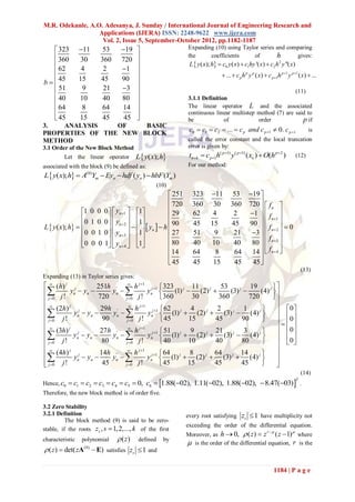
Problem 1 This problem was solved by [12] and [4].
Consider a linear first order IVP: They adopted block methods of order four to solve
y '   y, y(0)  1, 0  x  2, h  0.1 (20) the problem (20). We compare the result of our
with the exact solution: new block method (9) (which is of order five) with
their results as shown in table 1 below.
y ( x)  e x (21)

Table 1: Performance of the New Block Method on y '   y, y(0)  1, 0  x  1, h  0.1
_____________________________________________________________________________________
x Exact solution Computed Solution ERR EOAS EMY
---------------------------------------------------------------------------------------------------------------------------------------
0.1000 0.9048374180359595 0.9048374025462963 1.5490(-08) 2.3231(-07) 2.5292(-06)
0.2000 0.8187307530779818 0.8187307437037037 9.3743(-09) 1.0067(-07) 2.0937(-06)
0.3000 0.7408182206817178 0.7408182037500000 1.6932(-08) 3.2505(-07) 2.0079(-06)
0.4000 0.6703200460356393 0.6703200296296297 1.6406(-08) 4.6622(-07) 1.6198(-06)
0.5000 0.6065306597126334 0.6065306344848305 2.5228(-08) 3.4071(-07) 3.1608(-06)
0.6000 0.5488116360940264 0.5488116163781553 1.9716(-08) 4.8161(-07) 2.7294(-06)
0.7000 0.4965853037914095 0.4965852802878691 2.3504(-08) 5.6328(-07) 2.5457(-06)
0.8000 0.4493289641172216 0.4493289421226676 2.1995(-08) 4.4956(-07) 2.1713(-06)
0.9000 0.4065696597405991 0.4065696328791496 2.6862(-08) 5.3518(-07) 3.1008(-06)
1.0000 0.3678794411714423 0.3678794189516900 2.2220(-08) 5.7870(-07) 2.7182(-06)
---------------------------------------------------------------------------------------------------------------------------------------
Problem 2 This problem was solved by [13] and [4].
Consider a linear first order IVP: They adopted a self-starting block method of order
y '  xy, y(0)  1, 0  x  2, h  0.1 (22) six and four respectively to solve the problem (22).
with the exact solution: We compare the result of our new block method (9)
(which is of order five) with their results as shown
x2
in table 2.
y ( x)  e 2 (23)
Table 2: Performance of the New Block Method on y '  xy, y(0)  1, 0  x  1, h  0.1
_____________________________________________________________________________________
x Exact solution Computed Solution ERR EOAS EBM
---------------------------------------------------------------------------------------------------------------------------------------
0.1000 1.0050125208594010 1.0050122069965277 3.1386(-07) 5.2398(-07) 5.29(-07)
0.2000 1.0202013400267558 1.0202011563888889 1.3364(-07) 1.6913(-07) 1.77(-07)
0.3000 1.0460278599087169 1.0460275417187499 3.1819(-07) 8.7243(-07) 8.99(-07)
0.4000 1.0832870676749586 1.0832870577777778 9.8972(-09) 3.0098(-06) 3.09(-06)
0.5000 1.1331484530668263 1.1331477578536935 6.9521(-07) 1.7466(-06) 1.91(-06)
0.6000 1.1972173631218102 1.1972169551828156 4.0794(-07) 4.1710(-06) 4.48(-06)
0.7000 1.2776213132048868 1.2776205400192113 7.7319(-07) 9.6465(-06) 1.02(-05)
0.8000 1.3771277643359572 1.3771270561253053 7.0821(-07) 6.7989(-06) 7.74(-05)
0.9000 1.4993025000567668 1.4992996318515335 2.8682(-06) 1.2913(-05) 1.44(-05)
1.0000 1.6487212707001282 1.6487192043043850 2.0664(-06) 2.6575(-05) 2.93(-05)
---------------------------------------------------------------------------------------------------------------------------------------

5. CONCLUSION natural laws of growth and decay. Pacific
In this paper, we have proposed a new 4- Journal of Science and Technology, 12(1),
point block numerical method for the solution of 237-243, 2011.
first-order ordinary differential equations. The block [2] P. Kandasamy, K. Thilagavathy and K.
integrator proposed was found to be zero-stable, Gunavathy, Numerical methods (S. Chand
consistent and convergent. The new method was also and Company, New Delhi-110 055, 2005).
found to perform better than some existing methods. [3] J. O. Ehigie, S. A. Okunugo, and A. B.
Sofoluwe, A generalized 2-step continuous
implicit linear multistep method of hybrid
type. Journal of Institute of Mathematics
References and Computer Science, 2(6), 362-372, 2010.
[1] J. Sunday, On Adomian decomposition [4] M. R. Odekunle, A. O. Adesanya and J.
method for numerical solution of ordinary Sunday, A new block integrator for the
differential equations arising from the solution of initial value problems of first-

1186 | P a g e

order ordinary differential equations, differential equation, Intern. J. Comp. Math,
International Journal of Pure and Applied 77, 117-124, 2001.
Science and Technology, 11(2), 92-100, [18] G. G. Dahlquist, Numerical integration of
2012. ordinary differential equations, Math.
[5] P. Onumanyi, D. O. Awoyemi, S. N. Jator Scand., 4(1), 33-50, 1956.
and U. W. Sirisena, New linear multistep
methods with continuous coefficients for
first Order IVPS, Journal of the Nigerian
Mathematical Society, 13, 37-51, 1994.
[6] W. E. Milne, Numerical solution of
differential equations (New York, Willey,
1953).
[7] J. B. Rosser, A Runge-Kutta method for all
Seasons. SIAM Review, 9, 417-452, 1967. .
[8] L. F. Shampine and H. A. Watts, Block
implicit one-step Methods, Mathematics of
Computation, 23(108), 731-740, 1969.
[9] J. C. Butcher, Numerical Methods for
Ordinary Differential Equation (West
Sussex: John Wiley & Sons, 2003).
[10] Zarina, B. I., Mohammed, S., Kharil, I. and
Zanariah, M, Block Method for Generalized
Multistep Adams Method and Backward
Differentiation Formula in solving first-
order ODEs, Mathematika, 25-33, 2005.
[11] D. O. Awoyemi, R. A. Ademiluyi and E.
Amuseghan, Off-grids exploitation in the
development of more accurate method for
the solution of ODEs, Journal of
Mathematical Physics, 12, 379-386, 2007.
[12] U. Mohammed, and Y. A. Yahaya, Fully
implicit four point block backward
difference formula for solving first-order
initial value problems, Leonardo Journal of
Sciences, 16(1) ,21-30, 2010.
[13] A. M. Badmus and D. W. Mishelia, Some
uniform order block method for the solution
of first-order ordinary differential equations,
Journal of Nigerian Association of
Mathematical Physics, 19 ,149-154, 2011.
[14] E. A. Areo, R. A. Ademiluyi, and P.O.
Babatola, Three steps hybrid linear multistep
method for the solution of first-order initial
value problems in ordinary differential
equations, Journal of Mathematical Physics,
19, 261-266, 2011.
[15] E. A. Ibijola, Y. Skwame and G. Kumleng,
Formulation of hybrid method of higher
step-sizes through the continuous multistep
collocation, American Journal of Scientific
and Industrial Research, 2, 161-173, 2011.
[16] J. P. Chollom, I. O. Olatunbosun, and S. A.
Omagu, A class of A-stable block explicit
methods for the solution of ordinary
differential equations. Research Journal of
Mathematics and Statistics, 4(2), 52-56,
2012.
[17] D. O. Awoyemi, A new sixth-order
algorithm for general second-order ordinary

1187 | P a g e

Gm2511821187

More Related Content

What's hot

Viewers also liked

Similar to Gm2511821187

Gm2511821187