Local Vibrational Modes

Local Mode Analysis
D Setiawan
Computational and Theoretical Chemistry Group Workshop
Southern Methodist University
dsetiawan@smu.edu
December 18, 2014
D Setiawan (CATCO Workshop) Local Mode Analysis December 18, 2014 1 / 41

Overview
1 Part I: Local Mode Analysis
2 Part II: Running the Local Mode Program
3 Part III: Bar Diagrams
4 Part IV: Adiabatic Connection Scheme

How to Measure a Chemical Bond Strength?
Bond Dissociation Energy (BDE)?
1532 Current Organic Chemistry, 2010, Vol. 14, No. 15 Cremer and Kraka
to an analysis of the reaction path direction and its curvature [115-
124].
molecules, especially when hetero atoms are involved, these
requirements are seldom fulfilled. However, even if the
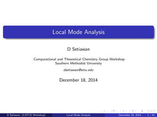
Fig. (2). Schematic representation of a Morse potential for the dissociation of the bond AB in HpA BHq. Bond dissociation energy BDE, intrinsic bond
dissociation energy IBDE, fragment stabilisation energy ES=EDR+EGR, density reorganization energy EDR, geometry relaxation energy EGR, and compressibility
limit distance dc are indicated.
D.Cremer & E. Kraka, Curr. Org. Chem., 2010, 14, 1524

How to Measure a Chemical Bond Strength?
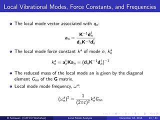
A Better Measure: Intrinsic BDE
1532 Current Organic Chemistry, 2010, Vol. 14, No. 15 Cremer and Kraka
to an analysis of the reaction path direction and its curvature [115-
124].
molecules, especially when hetero atoms are involved, these
requirements are seldom fulfilled. However, even if the
requirements would be fulfilled, the bond order defined in this way
Fig. (2). Schematic representation of a Morse potential for the dissociation of the bond AB in HpA BHq. Bond dissociation energy BDE, intrinsic bond
dissociation energy IBDE, fragment stabilisation energy ES=EDR+EGR, density reorganization energy EDR, geometry relaxation energy EGR, and compressibility
limit distance dc are indicated.
D.Cremer & E. Kraka, Curr. Org. Chem., 2010, 14, 1524

Vibrational Spectroscopy: A Tool for Measuring IBDE
Molecular vibrations can probe the strength of chemical bonds
Vibrational frequency and force constant of a stretching vibration is
related to the bond strength
Problem:
Normal vibrational modes are always delocalized as a result of
kinematic coupling (mass-coupling)
e.g. mode-mode couplings among stretching + bending + torsion
modes
Consequences:
Normal modes from IR/Raman spectrums are not useful in describing
chemical bonding
informations are diﬃcult to decipher in terms of internal parameter
modes, e.g. a particular stretching mode

Solution: Local Vibrational Modes
Normal modes are only electronically decoupled and therefore they are
still delocalized & cannot describe an individual (local) bond.
There have been many eﬀorts to derive a “local” vibrational modes
(see D.Cremer & E. Kraka, Curr. Org. Chem., 2010, 14, 1524)

Part I : Local Mode Analysis

Konkoli-Cremer Local Vibrational Modes
Solving mass-decoupled Euler-Lagrange equations, driven by changes
in an associated internal coordinate:
setting all masses equal to zero with the exception of those of the
molecular fragment (e.g., bond AB)
It’s been proved that this is equivalent to requiring the adiabatic
relaxation of the rest of the molecule after displacement of the
speciﬁc internal coordinates (e.g., bond AB)
Z. Konkoli & D. Cremer, Int. J. Quant. Chem., 1998, 67, 1

Normal Vibrational Frequencies (1)
Vibrational secular equation expressed in Cartesian coordinates:
Fx
L = MLΛ
Fx
, force constant matrix
L, collections of (re-normalized) normal vibrational eigenvectors, lµ
M, mass matrix
Λ, diagonal matrix with eigenvalues λµ = (2πcω)2

Normal Vibrational Frequencies (2)
Vibrational secular equation expressed in internal coordinates:
Fq
D = G−1
DΛ
Fq
, force constant matrix (in terms of internal coordinates, qn)
D, collections of (re-normalized) normal vibrational eigenvectors, dµ
G, Wilson matrix; gives kinetic energy in terms of internal coordinates
Λ, diagonal matrix with eigenvalues λµ = (2πcω)2

Cartesian & Internal Coordinates
Relationship between L and D:
L = CD
C is pseudo-inverse of B matrix;
B is ﬁrst derivatives matrix of internal coordinates qn w.r.t. Cartesian
coordinates:
C = M−1
B†
G−1
in which:
Bni =
∂qn(x)
∂xi x=x0

Some Important Relationships...
Normalization Cartesian Internal Equals to:
Coordinates Coordinates
Normalized
˜L†M˜L ˜D†G−1 ˜D I
˜L†Fx˜L ˜D†Fq ˜D Λ
Re-normalized
L†ML D†G−1D MR
L†FxL D†FqD K
K, is the diagonal normal force constant matrix
MR, is the reduced mass matrix, which elements are the
re-normalization constant MR
µ = 1
˜l†
µ
˜lµ
; i.e.
L = ˜L(MR
)
1
2

Local Vibrational Modes, Force Constants, and Frequencies
The local mode vector associated with qn:
an =
K−1d†
n
dnK−1d†
n
The local mode force constant ka of mode n, ka
n
ka
n = a†
nKan = (dnK−1
d†
n)−1
The reduced mass of the local mode an is given by the diagonal
element Gnn of the G matrix.
Local mode mode frequency, ωa:
(ωa
n)2
=
1
(2πc)2
ka
nGnn

Part II: Running the Local Mode Program

Setting-up The Local Mode Program @ SMUHPC-3
Set-up The Local-Mode Program
export PATH=/users/chem/Software/ALM:$PATH
Set-up The Local-Mode Analysis Script
export PATH=/users/chem/Software/Python/bin/python:$PATH
alias alm-analysis=’python /users/chem/Software/ALM-scripts/local mode analysis.py’

Running The Local Mode Program
General Syntax
alm.exe -b <input.alm >output.alm.out

The Local Mode Program: Input Keywords
The manual is available at
SMUHPC:/users/chem/Software/ALM/manual
The example ﬁles at:
/users/chem/Software/ALM/CATCO-Workshop/
CONTROL
$contrl
qcprog=”ProgramName”
iprint=2
iredun=1
isymm=1
$end

The Local Mode Program: Input Keywords
DATA
$qcdata
fchk=”ﬁlename.type”
$end
LOCAL MODE DESCRIPTIONS
$LocMod $End
2 1 0 0 PP
2 1 5 0 PPH
7 2 1 5 HPPH

Output: Local Mode Frequencies, Force Const., etc.

Output: Normal Mode Decomposition

Part III: Bar Diagrams

Bar Diagrams
Normal Mode Decomposition Bar Diagram:
The decomposition of each normal modes into its local mode
components
Inverted Bar Diagram:
Possible association of local modes to multiple diﬀerent normal modes
Important Notes: For creating Bar Diagrams and Adiabatic
Connection Scheme (ACS), complete set of (3N-6) internal modes
need to be supplied!

Bar Diagram from ALM Analysis Scripts: Syntaxes
Normal Mode Decomposition Bar Diagram Syntax
alm-analysis output.alm.out
alm-analysis output.alm.out “1,3”
alm-analysis output.alm.out 1
Inverted Bar Diagram Syntax
alm-analysis output.alm.out

Bar Diagram from ALM Analysis Scripts: Output
The numerical argument in the syntax represent the modes to be
highlighted (yellow-colored)
Highlight mode has not yet implemented for the Inverted Bar Diagram
Output: Bar Diagrams (PDF), Normal Modes Decomposition Table
(TeX)

Normal Mode Decomposition Bar Diagram

Normal Mode Decomposition (Highlighted)

Inverted Bar Diagram

Part IV: Adiabatic Connection Scheme

Adiabatic Connection Scheme (ACS)
Demonstrating the relationship of normal and local vibrational modes
Gives information about mass-coupling between local modes
Expressed in Decius’ compliance constants, Γn = 1
ka
n
:
(Γq
)−1 ˜D = G−1 ˜DΛ
G˜R = Γq ˜RΛ
which then matrix Γq
and G can be partitioned into its diagonal and
off-diagonal parts:
(Gd + λGod)˜Rλ = (Γq
d + λΓq
od)˜RλΛλ
The off-diagonal parts can be switched off by choosing scaling factor
λ = 0, thus a local (adiabatic) mode description is given.

ACS from ALM Analysis Scripts: Syntaxes
Adiabatic Connection Scheme Syntax
alm-analysis output.alm.out job-ACSF.dat N
N = number of ACS plots to be made (i.e. division into diﬀerent
frequency regions), default N = 1

ACS: Lower Frequencies Region
0.0 0.1 0.2 0.3 0.4 0.5 0.6 0.7 0.8 0.9 1.0
Scaling Factor λ
0
150
300
450
600
750
900
1050
1200
LocalModeFrequenicesωa[cm−1
]
NormalModeFrequenciesωµ[cm−1
]
ωa(11),ωa(10),ωa(18)
ωa(8),ωa(9),ωa(1)
ωa(6),ωa(7)
ωa(15),ωa(16),ωa(14),ωa(17)
ωa(12),ωa(13)
ω1(Bu),ω2(Ag),ω3(Au)
ω4(Au),ω5(Bg)
ω6(Ag)
ω7(Bu),ω8(Ag)
ω9(Au),ω10(Bu),ω11(Bg)
ω12(Ag),ω13(Ag)
ω14(Bu)
pnicogen

ACS: High Frequencies Region
0.0 0.1 0.2 0.3 0.4 0.5 0.6 0.7 0.8 0.9 1.0
Scaling Factor λ
2412
2416
2420
2424
2428
2432
2436
2440
2444
LocalModeFrequenicesωa[cm−1
]
NormalModeFrequenciesωµ[cm−1
]
ωa(3),ωa(2),ωa(5),ωa(4)
ω15(Ag)
ω16(Bu)
ω17(Bg)
ω18(Au)
pnicogen

ACS Analysis from the ALM Scripts: Output
Output: ACS Plot(s) (PDF), Normal Modes Decomposition Table
(TeX), ACS Table (TeX)
The job-ACSF.dat ﬁle can also be plotted with DataGraph for a
publication-quality plots

ACS DataGraph: Low Frequencies Region
NormalModeFrequenciesωμ[cm-1
]
P1
H7 H5
F3 P2
H6H8
F4
ω1(Bu)
ω2(Ag)ω3(Au)
ω6(Ag)
ω5(Bg)
ω4(Au)
P2 P1
F4-P2 P1
F3-P1 P2
F3-P1 P2-F4
H8-P2 P1
H5-P1 P2
A.C.
LocalModeFrequenciesωa
[cm-1
]
100
200
300
400
500
Scaling Factor λ
0 0.1 0.2 0.3 0.4 0.5 0.6 0.7 0.8 0.9 1.0

ACS DataGraph: Mid Frequencies Region
]
P1
H7 H5
F3 P2
H6H8
F4
ω8(Ag)ω7(Bu)
ω9(Au)
ω11(Bg)
ω10(Bu)
ω12(Ag)ω13(Ag)
ω14(Bu)
F4-P2
F3-P1
H-P-F
H-P-H
[cm-1
]
800
900
1000
1100
Scaling Factor λ
0 0.1 0.2 0.3 0.4 0.5 0.6 0.7 0.8 0.9 1.0

ACS DataGraph: High Frequencies Region
]
P1
H7 H5
F3 P2
H6H8
F4
ω15(Ag)ω16(Bu)
ω18(Au)
ω17(Bg)
H-P
[cm-1
]
2420
2430
2440
Scaling Factor λ
0 0.1 0.2 0.3 0.4 0.5 0.6 0.7 0.8 0.9 1.0

Complete Set of Internal Modes
General rules: N bonds, (N-1) bond angles, (N-2) bond dihedrals
We have to account for each unique internal coordinate.
For the high symmetry systems this is easy;
For the low symmetry systems one has to run the job twice or 3
times and replace the coordinates to get all unique force constants.
This can be particularly tedious for ring molecules where we have to
make more than one (extra) run.

Complete Set of Internal Modes
One must not violate some redundancy rules:
In a planar system, we must give angles that add up to 360◦
The third angle must be used in a second run after replacing one of the
previous ones.
The same holds for the 6 angles of a tetrahedral center.
If one needs the 6th
angle, another angle must be replaced by this
angle in a second run.
In 5-ring systems we can only take 2 ring bendings and 2 ring torsions
at a time (N-3) so that the 5th ring bending angle has to be done in a
2nd run.
With curvilinear coordinates this would be straightforward, however
there are no curvilinear coordinates in the force ﬁeld program yet.
Hence they need all unique bending and torsional constants of the
ring.

Questions?

Exercises
SMUHPC-3:
/users/chem/Software/ALM/CATCO-Workshop/exercises
Comparing the local mode analysis results:
Do local mode analysis for pnicogen dimer calculated at CCSD(T) level
with CFOUR
Do another local mode analysis for pnicogen dimer calculated at DFT
level, corrected with the CCSD(T) frequencies
Compare the two results
Do the local mode analysis (include the ACS plots and Bar Diagrams)
for: Acetic Acid & Maleic Anhydride
C2
C1
H6
H8
H7
O4O3
H5
C5 C4
C2
O1
C3
O6O7
H9 H8

Hints: Input Keywords
DATA, Program=”CFour”
$qcdata
fchk=”CFOUR.out”
$end
Experimental Freq.
$ExpFreq MODE=1 $End
1 78.0408 Bu
2 94.6217 Ag
3 113.7508 Au

Local Vibrational Modes

More Related Content

What's hot

Viewers also liked

Similar to Local Vibrational Modes

Recently uploaded

Local Vibrational Modes