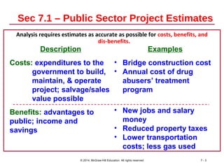
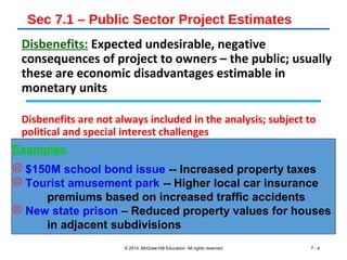
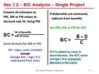
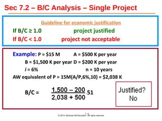
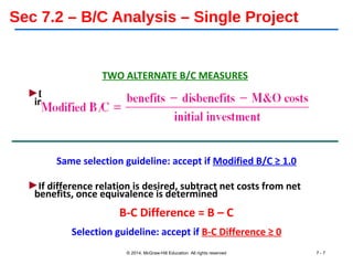
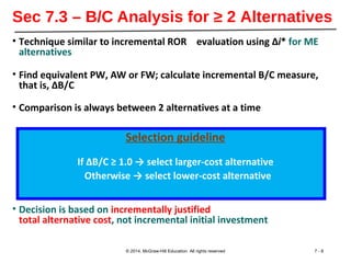
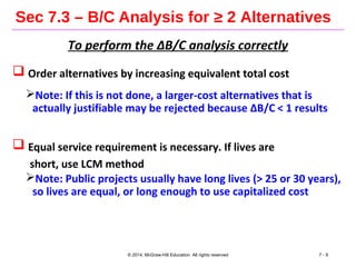
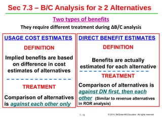
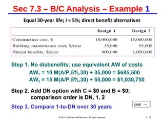
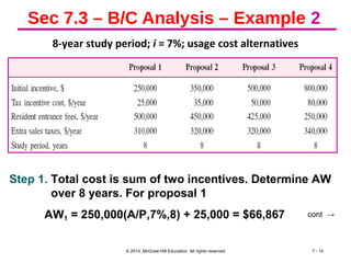
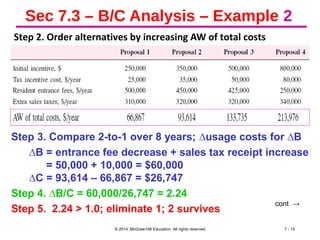
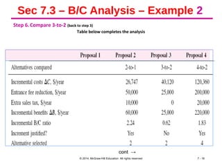
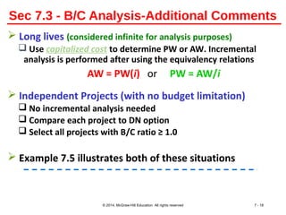
© 2014, McGraw-Hill Education All rights reserved7 - 1
Slides to accompany Blank and Tarquin
Basics of Engineering Economy, 2nd
ed.
Basics of Engineering Economy
by
Leland Blank and Anthony Tarquin
Slides to accompanySlides to accompany
Chapter 7
Benefit/Cost Analysis
and Public Sector Projects
Chapter 7 – Benefit/Cost Analysis
PURPOSE
Learn about
and perform a benefit/cost
analysis
TOPICS
B/C analysis of single project
B/C analysis of 2 or more
alternatives
© 2014, McGraw-Hill Education All rights reserved7 - 2
Sec 7.1 – Public Sector Project Estimates
Analysis requires estimates as accurate as possible for costs, benefits, and
dis-benefits.
© 2014, McGraw-Hill Education All rights reserved 7 - 3
Description
Costs: expenditures to the
government to build,
maintain, & operate
project; salvage/sales
value possible
Benefits: advantages to
public; income and
savings
Examples
• Bridge construction cost
• Annual cost of drug
abusers’ treatment
program
• New jobs and salary
money
• Reduced property taxes
• Lower transportation
costs; less gas used
Sec 7.1 – Public Sector Project Estimates
Disbenefits: Expected undesirable, negative
consequences of project to owners – the public; usually
these are economic disadvantages estimable in
monetary units
Disbenefits are not always included in the analysis; subject to
political and special interest challenges
© 2014, McGraw-Hill Education All rights reserved 7 - 4
Examples
 $150M school bond issue -- Increased property taxes
 Tourist amusement park -- Higher local car insurance
premiums based on increased traffic accidents
 New state prison – Reduced property values for houses
in adjacent subdivisions
Sec 7.2 – B/C Analysis – Single Project
Convert all estimates to
PW, AW or FW values at
discount rate i%. Using PW
PW of benefits
PW of costs
Same formula for AW or FW
All + signs, costs included
exceptexcept
Salvage has – sign; it is
subtracted from costs
If disbenefits are estimated,
subtract from benefits
Use PW, AW or FW for B/C
If D is added to costs in
denominator, the B/C value
changes, but economic
decision is the same
© 2014, McGraw-Hill Education All rights reserved 7 - 5
Sec 7.2 – B/C Analysis – Single Project
Guideline for economic justification
If B/C ≥ 1.0 project justified
If B/C < 1.0 project not acceptable
Example: P = $15 M A = $500 K per year
B = $1,500 K per year D = $200 K per year
i = 6% n = 10 years
AW equivalent of P = 15M(A/P,6%,10) = $2,038 K
B/C = = 0.51
© 2014, McGraw-Hill Education All rights reserved
7 - 6
Sec 7.2 – B/C Analysis – Single Project
TWO ALTERNATE B/C MEASURES
►Determine PW, AW or FW equivalent; denominator is only
initial investment with any salvage estimate
Same selection guideline: accept if Modified B/C ≥ 1.0
►If difference relation is desired, subtract net costs from net
benefits, once equivalence is determined
B-C Difference = B – C
Selection guideline: accept if B-C Difference ≥ 0
© 2014, McGraw-Hill Education All rights reserved 7 - 7
Sec 7.3 – B/C Analysis for ≥ 2 Alternatives
• Technique similar to incremental ROR evaluation using ∆i* for ME
alternatives
• Find equivalent PW, AW or FW; calculate incremental B/C measure,
that is, ∆B/C
• Comparison is always between 2 alternatives at a time
Selection guideline
If ∆B/C ≥ 1.0 → select larger-cost alternative
Otherwise → select lower-cost alternative
• Decision is based on incrementally justified
total alternative cost, not incremental initial investment
© 2014, McGraw-Hill Education All rights reserved 7 - 8
Sec 7.3 – B/C Analysis for ≥ 2 Alternatives
To perform the ∆B/C analysis correctly
 Order alternatives by increasing equivalent total cost
Note: If this is not done, a larger-cost alternatives that is
actually justifiable may be rejected because ∆B/C < 1 results
 Equal service requirement is necessary. If lives are
short, use LCM method
Note: Public projects usually have long lives (> 25 or 30 years),
so lives are equal, or long enough to use capitalized cost
© 2014, McGraw-Hill Education All rights reserved 7 - 9
Sec 7.3 – B/C Analysis for ≥ 2 Alternatives
Two types of benefits
They require different treatment during ∆B/C analysis
© 2014, McGraw-Hill Education All rights reserved7 - 10
USAGE COST ESTIMATES
DEFINITION
Implied benefits are based
on difference in cost
estimates of alternatives
TREATMENT
Comparison of alternatives
is against each other only
DIRECT BENEFIT ESTIMATES
DEFINITION
Benefits are actually
estimated for each alternative
TREATMENT
Comparison of alternatives is
against DN first, then each
other (Similar to revenue alternatives
in ROR analysis)
Sec 7.3-B/C Analysis for ≥ 2 ME Alternatives
PROCEDURE FOR ∆B/C OF MUTUALLY EXCLUSIVE ALTERNATIVES
1. Determine equivalent value for costs, benefits (and
disbenefits, if estimated)
2. Order alternatives by increasing total equivalent cost (for
direct benefit alternatives, add DN first)
3. For each pair of alternatives (call them 2 and 1), determine
incremental C and B over LCM. For usage cost alternative,
∆B = usage cost2 – usage cost1
4. Determine ∆B/C or ∆(B-D)/C
5. If ∆B/C ≥ 1.0, B is survivor; otherwise, A is survivor
6. Compare survivor with next alternative; continue steps (3) –
(5) until only 1 alternative remains
© 2014, McGraw-Hill Education All rights reserved7 - 11
Sec 7.3 – B/C Analysis – Example 1
Equal 30-year life; i = 5%; direct benefit alternatives
© 2014, McGraw-Hill Education All rights reserved 7 - 12
Step 1. No disbenefits; use equivalent AW of costs
AW1 = 10 M(A/P,5%,30) + 35,000 = $685,500
AW2 = 15 M(A/P,5%,30) + 55,000 = $1,030,750
Step 2. Add DN option with C = $0 and B = $0;
comparison order is DN, 1, 2
Step 3. Compare 1-to-DN over 30 years
cont →
Sec 7.3 – B/C Analysis – Example 1
Step 4. ∆B/C = 800,000/685,500 = 1.17
Step 5. 1.17 > 1, eliminate DN; 1 is survivor
Step 6. Compare 2-to-1 (back to step 3)
Step 3. Compare 2-to-1
∆B = 1,050,000 – 800,000 = $250,000
∆C = 1,030,750 – 685,500 = $345,250
Step 4. ∆B/C = 250,000/345,250 = 0.72
Step 5. 0.72 < 1, eliminate 2; 1 is survivor
Step 6. Select design 1
© 2014, McGraw-Hill Education All rights reserved 7 - 13
Sec 7.3 – B/C Analysis – Example 2
8-year study period; i = 7%; usage cost alternatives
© 2014, McGraw-Hill Education All rights reserved 7 - 14
cont →
Step 1. Total cost is sum of two incentives. Determine AW
over 8 years. For proposal 1
AW1 = 250,000(A/P,7%,8) + 25,000 = $66,867
Sec 7.3 – B/C Analysis – Example 2
Step 2. Order alternatives by increasing AW of total costs
© 2014, McGraw-Hill Education All rights reserved 7 - 15
cont →
Step 3. Compare 2-to-1 over 8 years; ∆usage costs for ∆B
∆B = entrance fee decrease + sales tax receipt increase
= 50,000 + 10,000 = $60,000
∆C = 93,614 – 66,867 = $26,747
Step 4. ∆B/C = 60,000/26,747 = 2.24
Step 5. 2.24 > 1.0; eliminate 1; 2 survives
Sec 7.3 – B/C Analysis – Example 2
Step 6.Compare 3-to-2 (back to step 3)
Table below completes the analysis
© 2014, McGraw-Hill Education All rights reserved 7 - 16
cont →
Sec 7.3 – B/C Analysis – Example 2
Results of comparisons
•Compare 3-to-2: ∆B/C = 25,000/40,120 = 0.62
Proposal 2 survives
•Compare 4-to-2: ∆B/C = 220,000/120,360 = 1.83
Proposal 2 eliminated; 4 survives
Conclusion: Select Proposal 4
© 2014, McGraw-Hill Education All rights reserved 7 - 17
Sec 7.3 - B/C Analysis-Additional Comments
 Long lives (considered infinite for analysis purposes)
 Use capitalized cost to determine PW or AW. Incremental
analysis is performed after using the equivalency relations
AW = PW(i) or PW = AW/i
 Independent Projects (with no budget limitation)
 No incremental analysis needed
 Compare each project to DN option
 Select all projects with B/C ratio ≥ 1.0
 Example 7.5 illustrates both of these situations
© 2014, McGraw-Hill Education All rights reserved 7 - 18

Lo4a(arif)

  • 1.
    © 2014, McGraw-HillEducation All rights reserved7 - 1 Slides to accompany Blank and Tarquin Basics of Engineering Economy, 2nd ed. Basics of Engineering Economy by Leland Blank and Anthony Tarquin Slides to accompanySlides to accompany Chapter 7 Benefit/Cost Analysis and Public Sector Projects
  • 2.
    Chapter 7 –Benefit/Cost Analysis PURPOSE Learn about and perform a benefit/cost analysis TOPICS B/C analysis of single project B/C analysis of 2 or more alternatives © 2014, McGraw-Hill Education All rights reserved7 - 2
  • 3.
    Sec 7.1 –Public Sector Project Estimates Analysis requires estimates as accurate as possible for costs, benefits, and dis-benefits. © 2014, McGraw-Hill Education All rights reserved 7 - 3 Description Costs: expenditures to the government to build, maintain, & operate project; salvage/sales value possible Benefits: advantages to public; income and savings Examples • Bridge construction cost • Annual cost of drug abusers’ treatment program • New jobs and salary money • Reduced property taxes • Lower transportation costs; less gas used
  • 4.
    Sec 7.1 –Public Sector Project Estimates Disbenefits: Expected undesirable, negative consequences of project to owners – the public; usually these are economic disadvantages estimable in monetary units Disbenefits are not always included in the analysis; subject to political and special interest challenges © 2014, McGraw-Hill Education All rights reserved 7 - 4 Examples  $150M school bond issue -- Increased property taxes  Tourist amusement park -- Higher local car insurance premiums based on increased traffic accidents  New state prison – Reduced property values for houses in adjacent subdivisions
  • 5.
    Sec 7.2 –B/C Analysis – Single Project Convert all estimates to PW, AW or FW values at discount rate i%. Using PW PW of benefits PW of costs Same formula for AW or FW All + signs, costs included exceptexcept Salvage has – sign; it is subtracted from costs If disbenefits are estimated, subtract from benefits Use PW, AW or FW for B/C If D is added to costs in denominator, the B/C value changes, but economic decision is the same © 2014, McGraw-Hill Education All rights reserved 7 - 5
  • 6.
    Sec 7.2 –B/C Analysis – Single Project Guideline for economic justification If B/C ≥ 1.0 project justified If B/C < 1.0 project not acceptable Example: P = $15 M A = $500 K per year B = $1,500 K per year D = $200 K per year i = 6% n = 10 years AW equivalent of P = 15M(A/P,6%,10) = $2,038 K B/C = = 0.51 © 2014, McGraw-Hill Education All rights reserved 7 - 6
  • 7.
    Sec 7.2 –B/C Analysis – Single Project TWO ALTERNATE B/C MEASURES ►Determine PW, AW or FW equivalent; denominator is only initial investment with any salvage estimate Same selection guideline: accept if Modified B/C ≥ 1.0 ►If difference relation is desired, subtract net costs from net benefits, once equivalence is determined B-C Difference = B – C Selection guideline: accept if B-C Difference ≥ 0 © 2014, McGraw-Hill Education All rights reserved 7 - 7
  • 8.
    Sec 7.3 –B/C Analysis for ≥ 2 Alternatives • Technique similar to incremental ROR evaluation using ∆i* for ME alternatives • Find equivalent PW, AW or FW; calculate incremental B/C measure, that is, ∆B/C • Comparison is always between 2 alternatives at a time Selection guideline If ∆B/C ≥ 1.0 → select larger-cost alternative Otherwise → select lower-cost alternative • Decision is based on incrementally justified total alternative cost, not incremental initial investment © 2014, McGraw-Hill Education All rights reserved 7 - 8
  • 9.
    Sec 7.3 –B/C Analysis for ≥ 2 Alternatives To perform the ∆B/C analysis correctly  Order alternatives by increasing equivalent total cost Note: If this is not done, a larger-cost alternatives that is actually justifiable may be rejected because ∆B/C < 1 results  Equal service requirement is necessary. If lives are short, use LCM method Note: Public projects usually have long lives (> 25 or 30 years), so lives are equal, or long enough to use capitalized cost © 2014, McGraw-Hill Education All rights reserved 7 - 9
  • 10.
    Sec 7.3 –B/C Analysis for ≥ 2 Alternatives Two types of benefits They require different treatment during ∆B/C analysis © 2014, McGraw-Hill Education All rights reserved7 - 10 USAGE COST ESTIMATES DEFINITION Implied benefits are based on difference in cost estimates of alternatives TREATMENT Comparison of alternatives is against each other only DIRECT BENEFIT ESTIMATES DEFINITION Benefits are actually estimated for each alternative TREATMENT Comparison of alternatives is against DN first, then each other (Similar to revenue alternatives in ROR analysis)
  • 11.
    Sec 7.3-B/C Analysisfor ≥ 2 ME Alternatives PROCEDURE FOR ∆B/C OF MUTUALLY EXCLUSIVE ALTERNATIVES 1. Determine equivalent value for costs, benefits (and disbenefits, if estimated) 2. Order alternatives by increasing total equivalent cost (for direct benefit alternatives, add DN first) 3. For each pair of alternatives (call them 2 and 1), determine incremental C and B over LCM. For usage cost alternative, ∆B = usage cost2 – usage cost1 4. Determine ∆B/C or ∆(B-D)/C 5. If ∆B/C ≥ 1.0, B is survivor; otherwise, A is survivor 6. Compare survivor with next alternative; continue steps (3) – (5) until only 1 alternative remains © 2014, McGraw-Hill Education All rights reserved7 - 11
  • 12.
    Sec 7.3 –B/C Analysis – Example 1 Equal 30-year life; i = 5%; direct benefit alternatives © 2014, McGraw-Hill Education All rights reserved 7 - 12 Step 1. No disbenefits; use equivalent AW of costs AW1 = 10 M(A/P,5%,30) + 35,000 = $685,500 AW2 = 15 M(A/P,5%,30) + 55,000 = $1,030,750 Step 2. Add DN option with C = $0 and B = $0; comparison order is DN, 1, 2 Step 3. Compare 1-to-DN over 30 years cont →
  • 13.
    Sec 7.3 –B/C Analysis – Example 1 Step 4. ∆B/C = 800,000/685,500 = 1.17 Step 5. 1.17 > 1, eliminate DN; 1 is survivor Step 6. Compare 2-to-1 (back to step 3) Step 3. Compare 2-to-1 ∆B = 1,050,000 – 800,000 = $250,000 ∆C = 1,030,750 – 685,500 = $345,250 Step 4. ∆B/C = 250,000/345,250 = 0.72 Step 5. 0.72 < 1, eliminate 2; 1 is survivor Step 6. Select design 1 © 2014, McGraw-Hill Education All rights reserved 7 - 13
  • 14.
    Sec 7.3 –B/C Analysis – Example 2 8-year study period; i = 7%; usage cost alternatives © 2014, McGraw-Hill Education All rights reserved 7 - 14 cont → Step 1. Total cost is sum of two incentives. Determine AW over 8 years. For proposal 1 AW1 = 250,000(A/P,7%,8) + 25,000 = $66,867
  • 15.
    Sec 7.3 –B/C Analysis – Example 2 Step 2. Order alternatives by increasing AW of total costs © 2014, McGraw-Hill Education All rights reserved 7 - 15 cont → Step 3. Compare 2-to-1 over 8 years; ∆usage costs for ∆B ∆B = entrance fee decrease + sales tax receipt increase = 50,000 + 10,000 = $60,000 ∆C = 93,614 – 66,867 = $26,747 Step 4. ∆B/C = 60,000/26,747 = 2.24 Step 5. 2.24 > 1.0; eliminate 1; 2 survives
  • 16.
    Sec 7.3 –B/C Analysis – Example 2 Step 6.Compare 3-to-2 (back to step 3) Table below completes the analysis © 2014, McGraw-Hill Education All rights reserved 7 - 16 cont →
  • 17.
    Sec 7.3 –B/C Analysis – Example 2 Results of comparisons •Compare 3-to-2: ∆B/C = 25,000/40,120 = 0.62 Proposal 2 survives •Compare 4-to-2: ∆B/C = 220,000/120,360 = 1.83 Proposal 2 eliminated; 4 survives Conclusion: Select Proposal 4 © 2014, McGraw-Hill Education All rights reserved 7 - 17
  • 18.
    Sec 7.3 -B/C Analysis-Additional Comments  Long lives (considered infinite for analysis purposes)  Use capitalized cost to determine PW or AW. Incremental analysis is performed after using the equivalency relations AW = PW(i) or PW = AW/i  Independent Projects (with no budget limitation)  No incremental analysis needed  Compare each project to DN option  Select all projects with B/C ratio ≥ 1.0  Example 7.5 illustrates both of these situations © 2014, McGraw-Hill Education All rights reserved 7 - 18