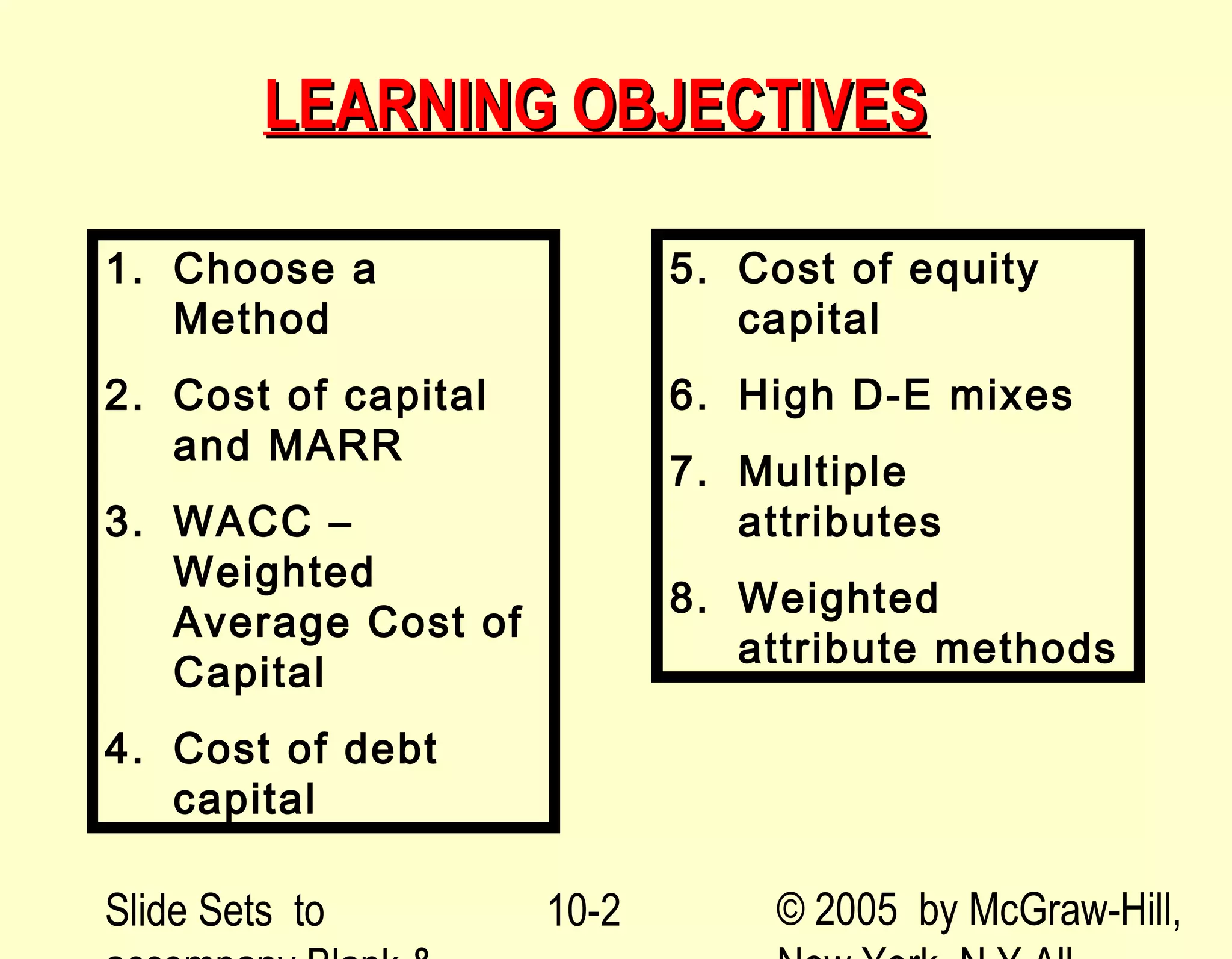
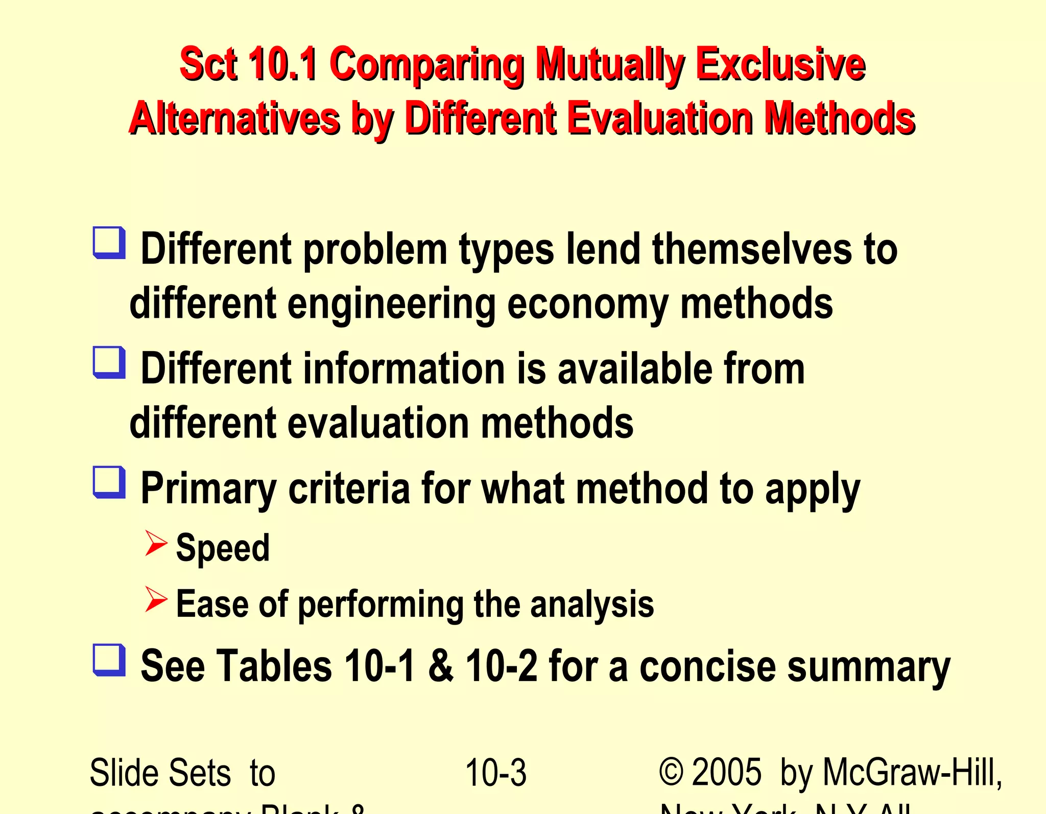
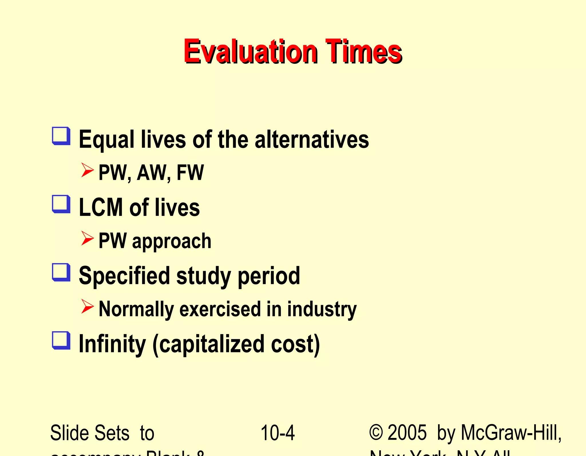
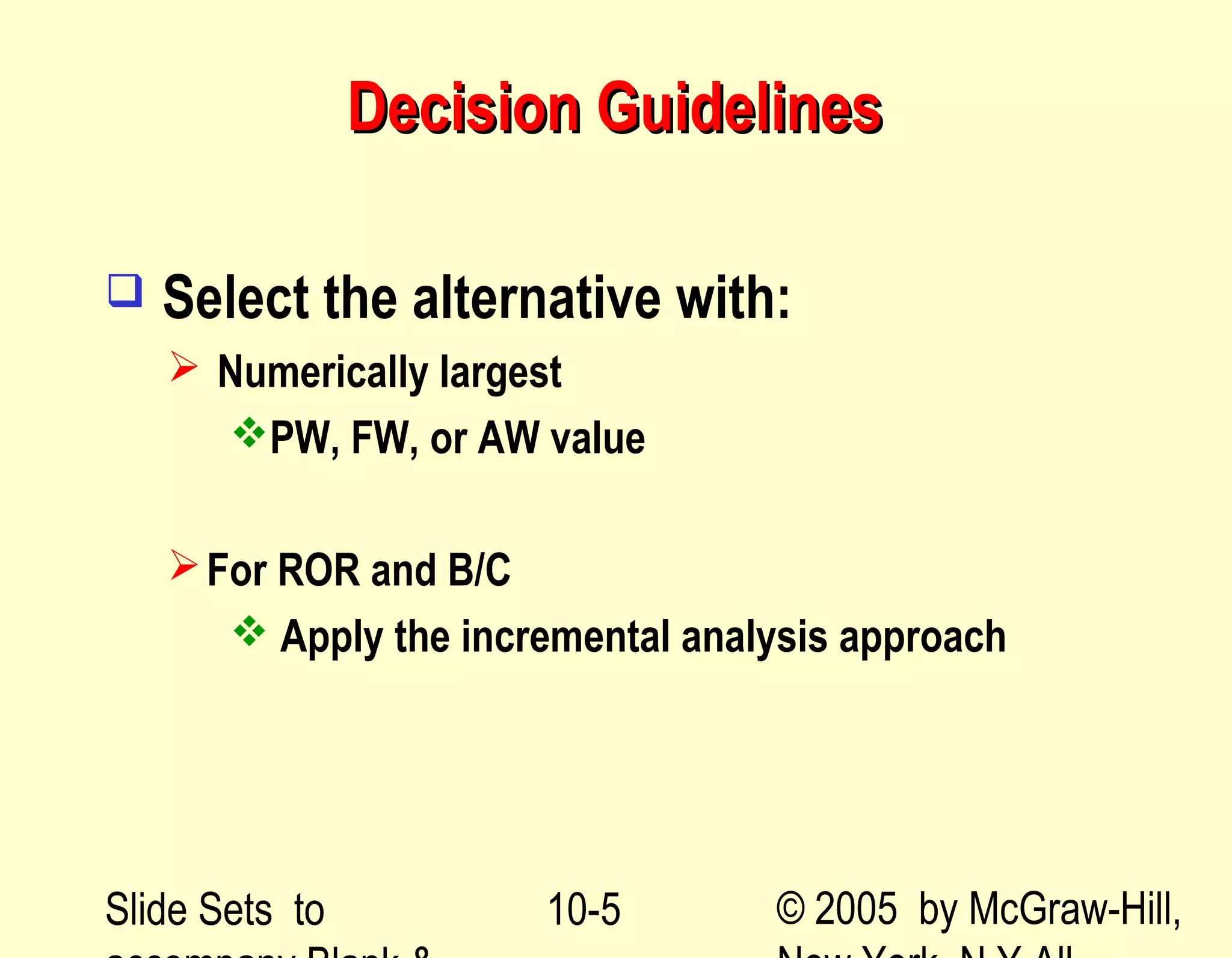
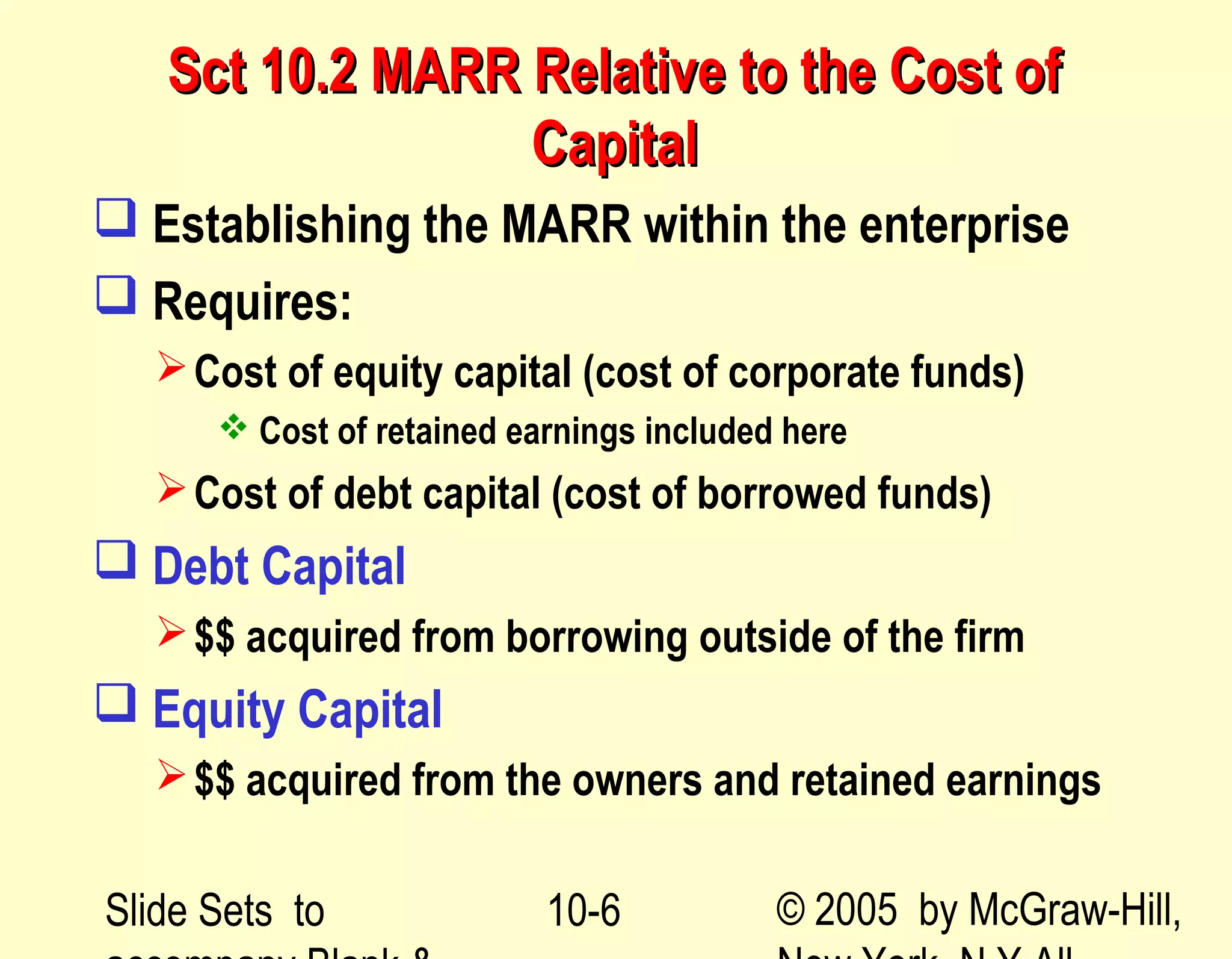
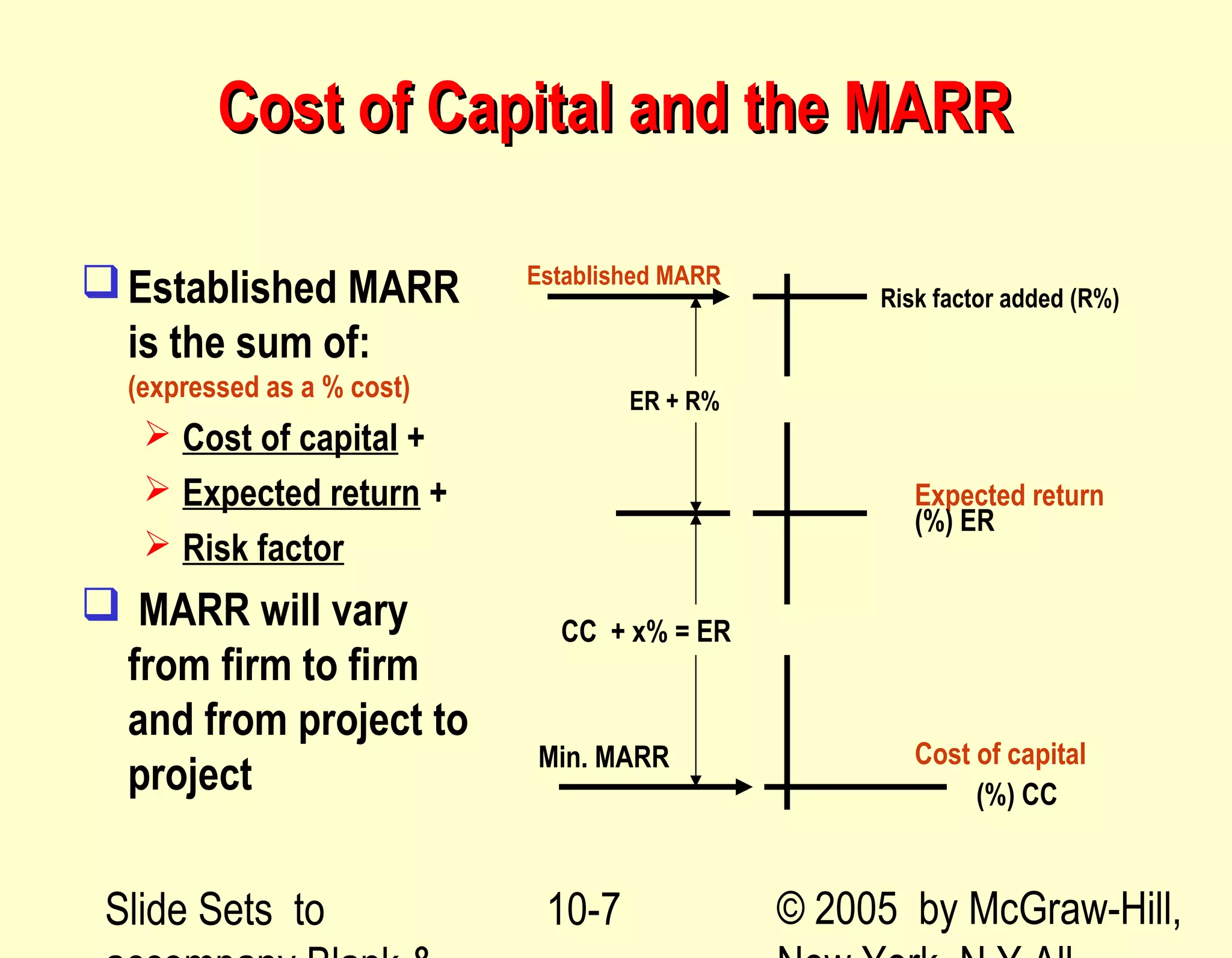
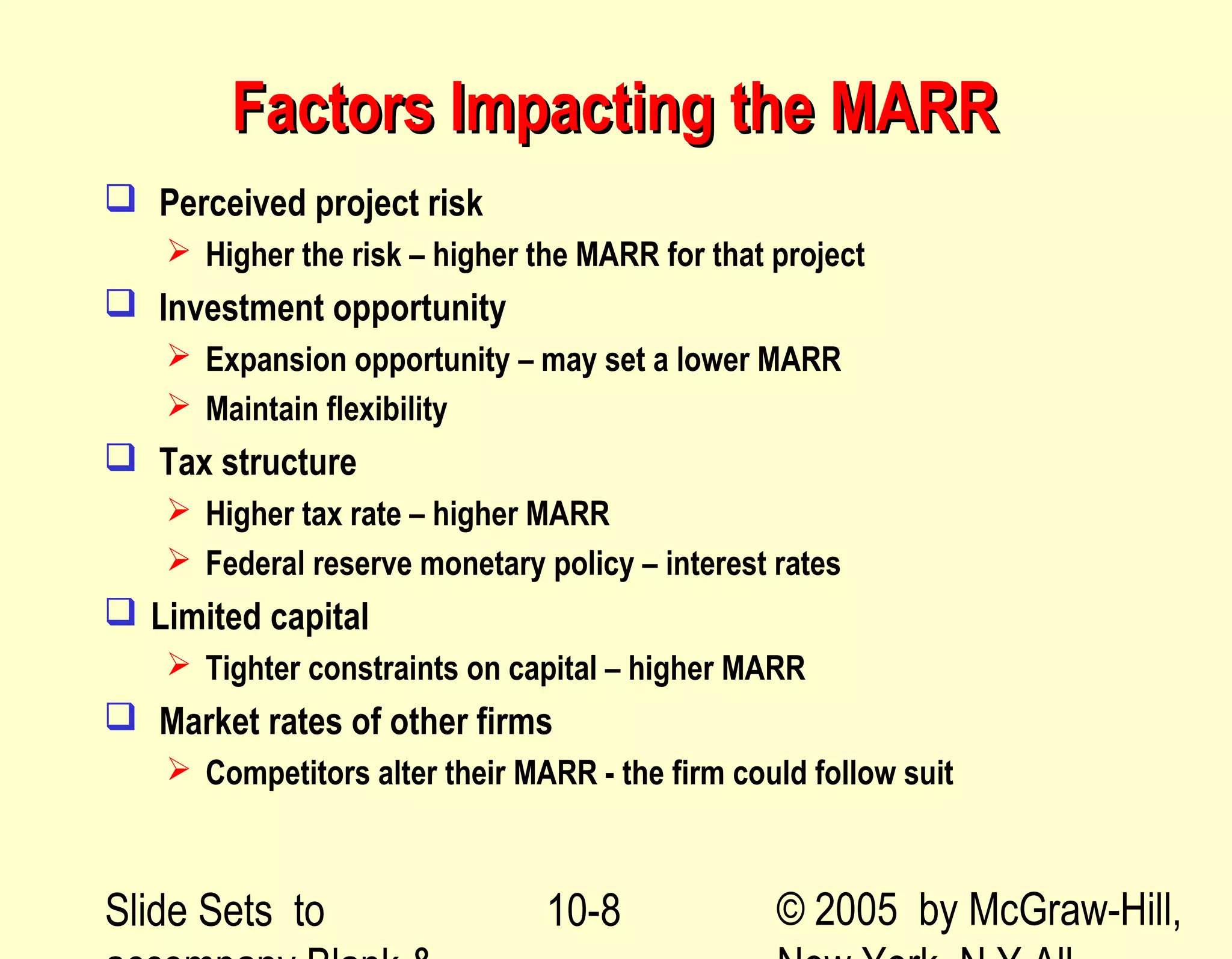
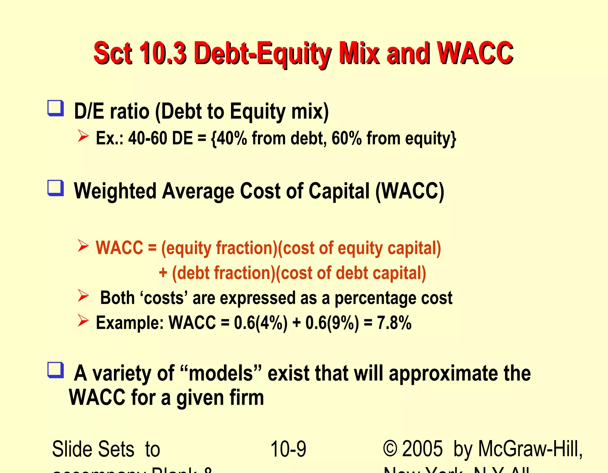
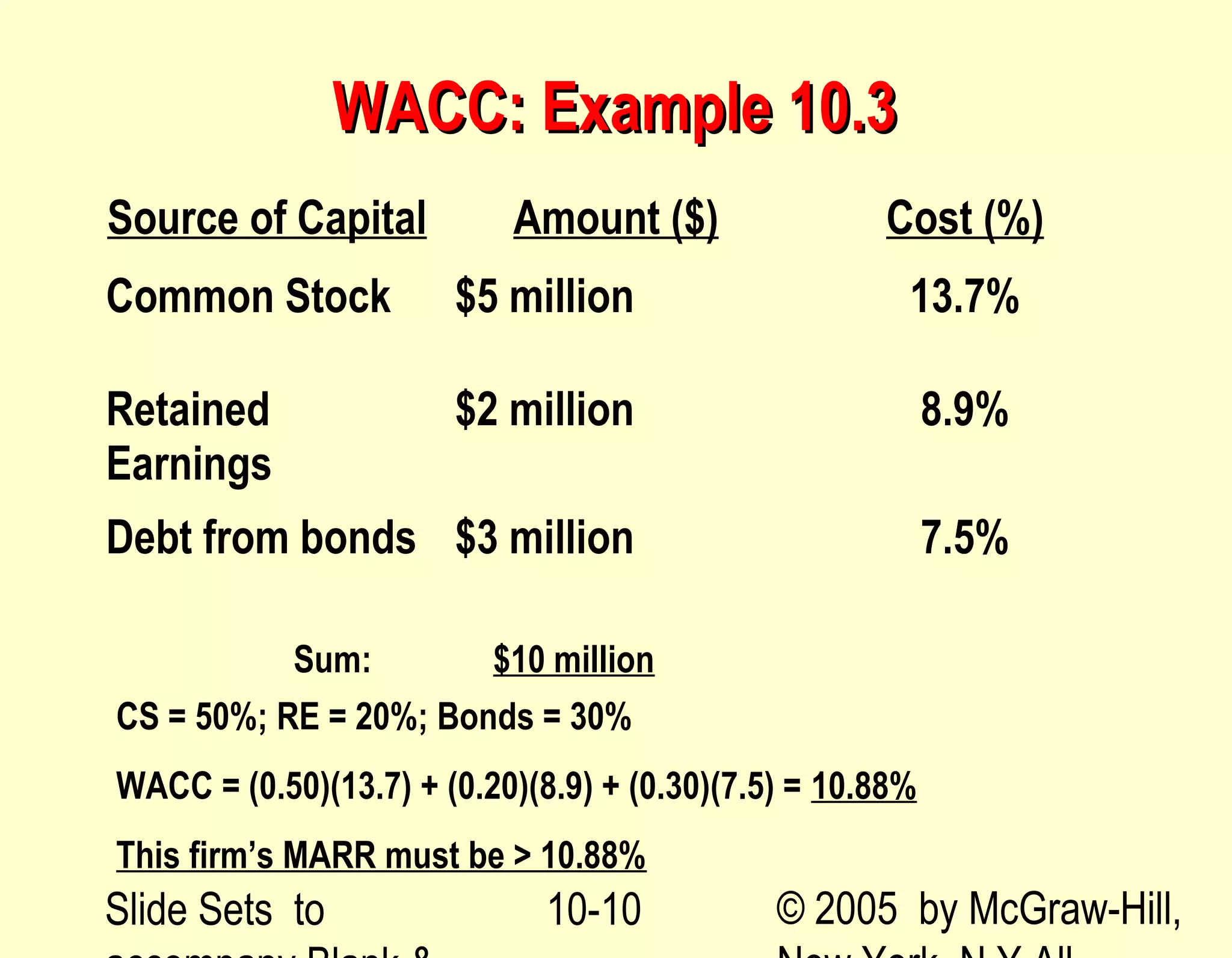
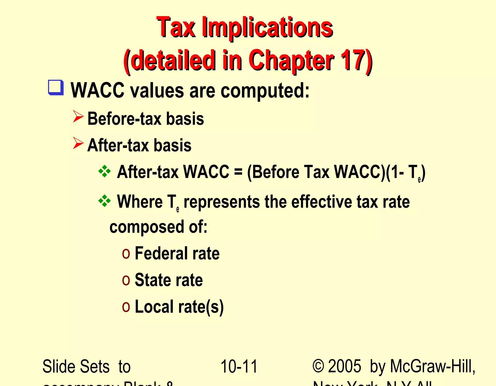
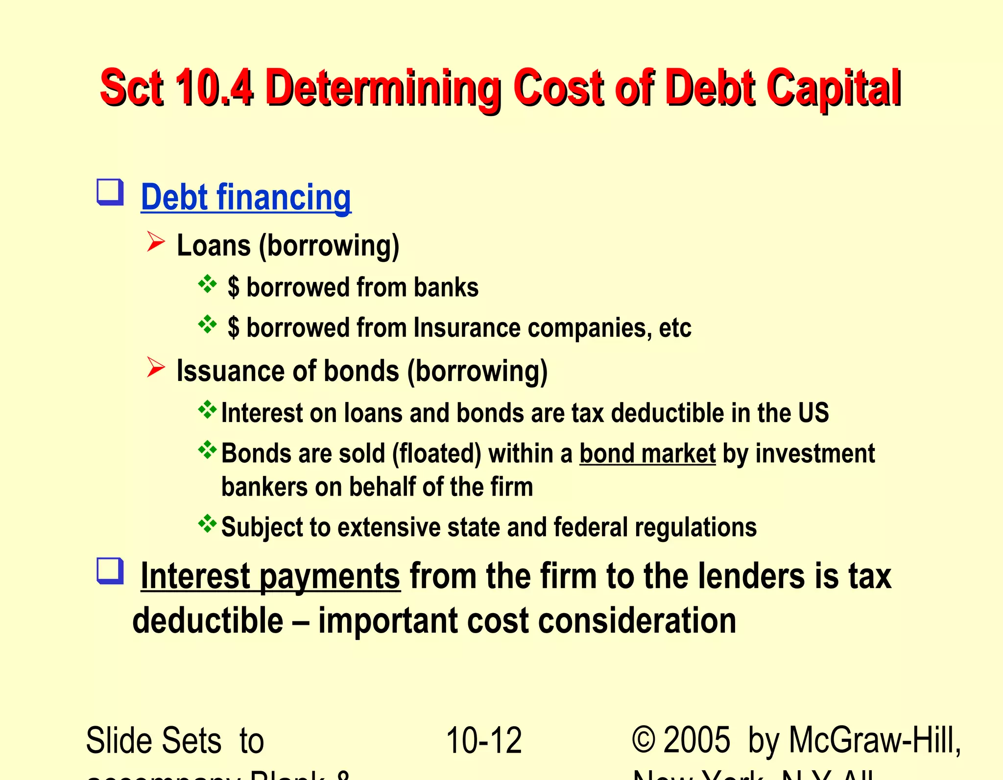
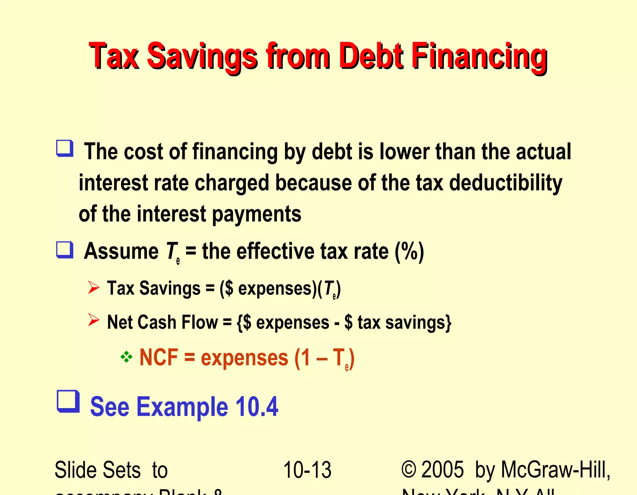
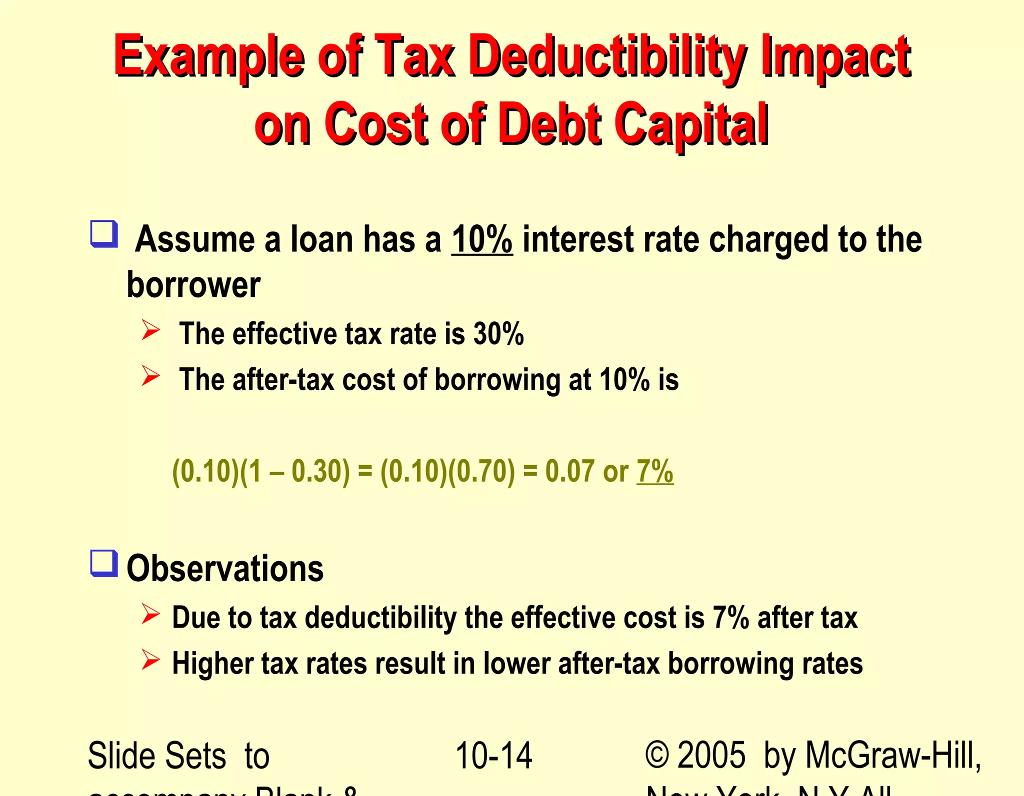
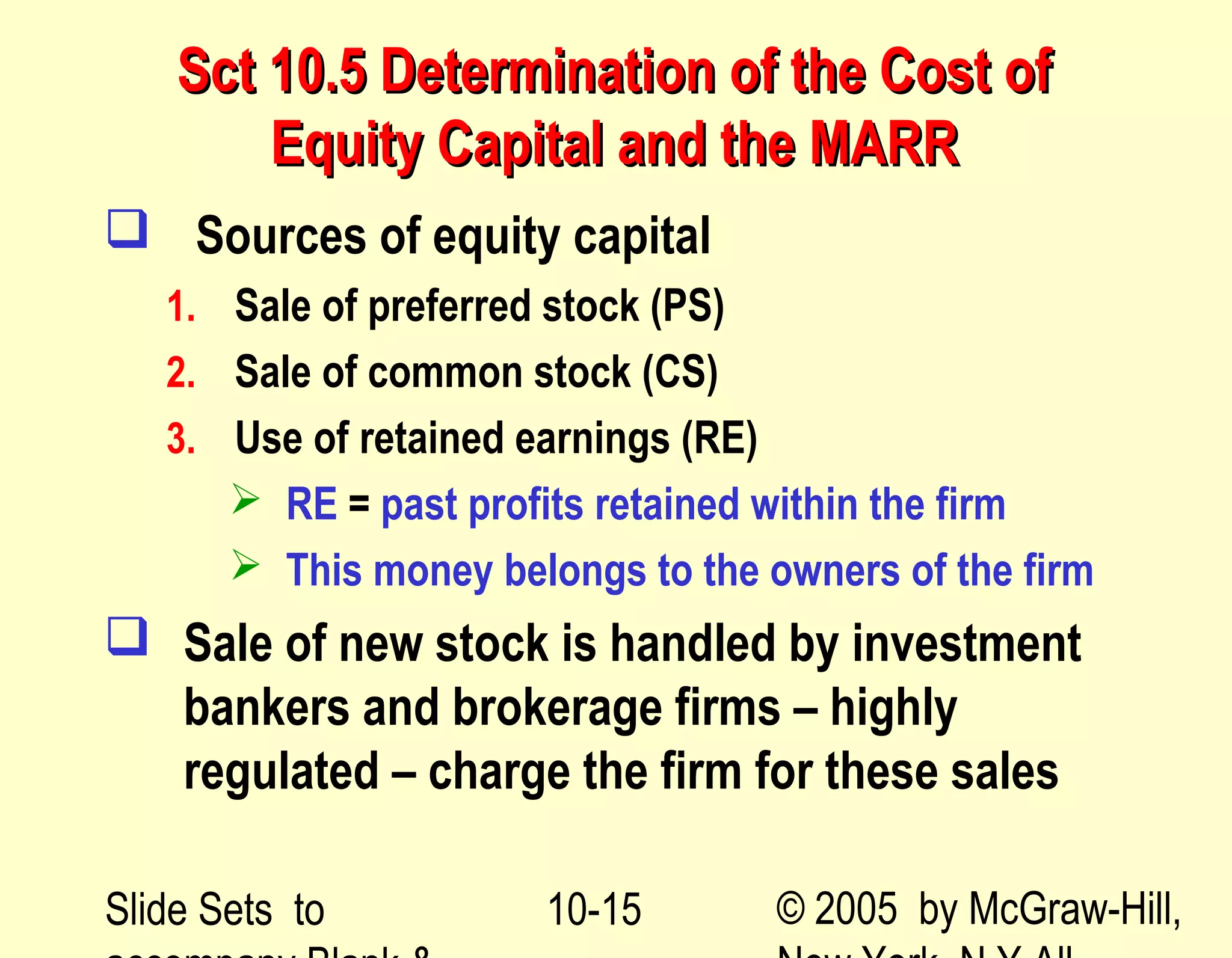
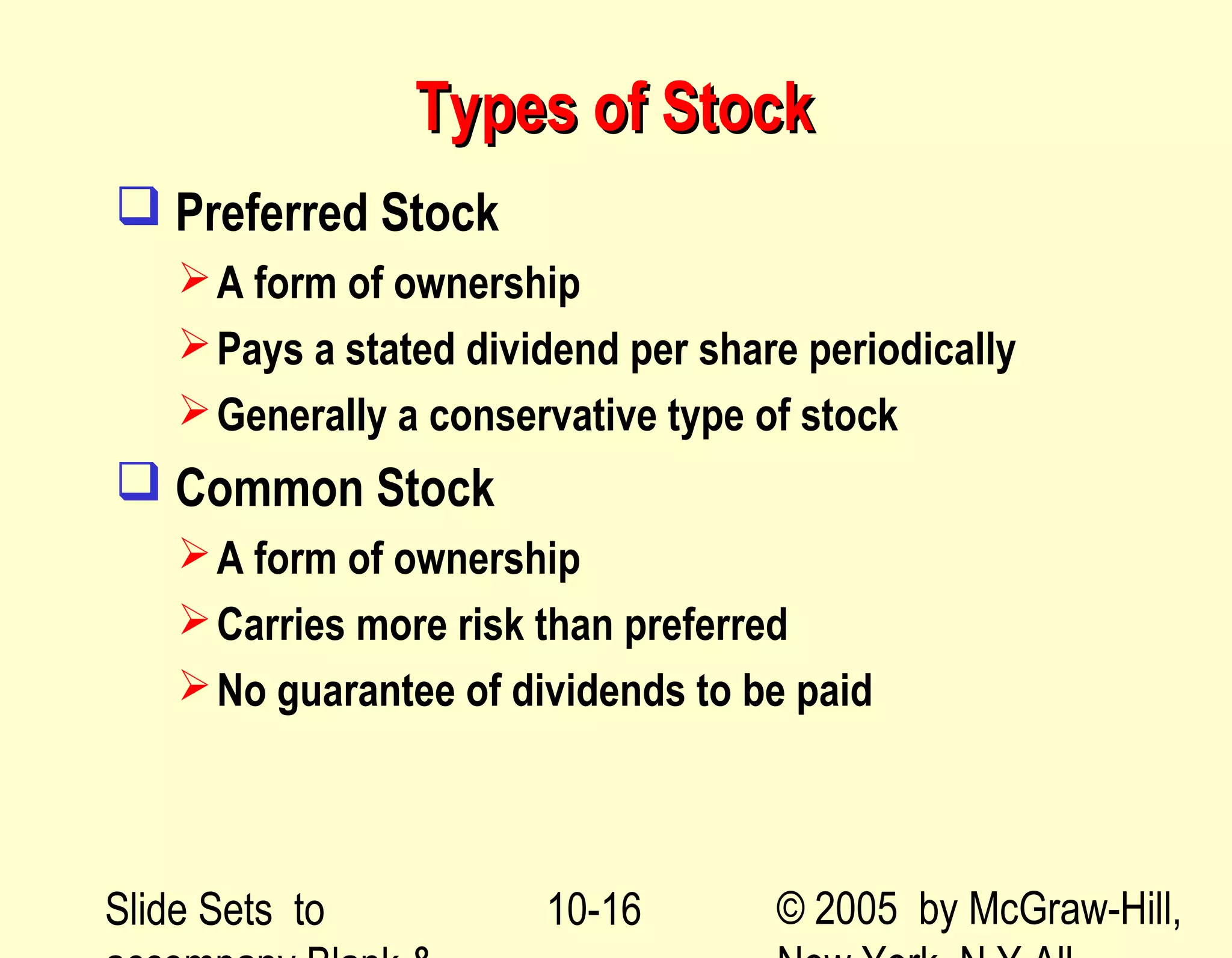
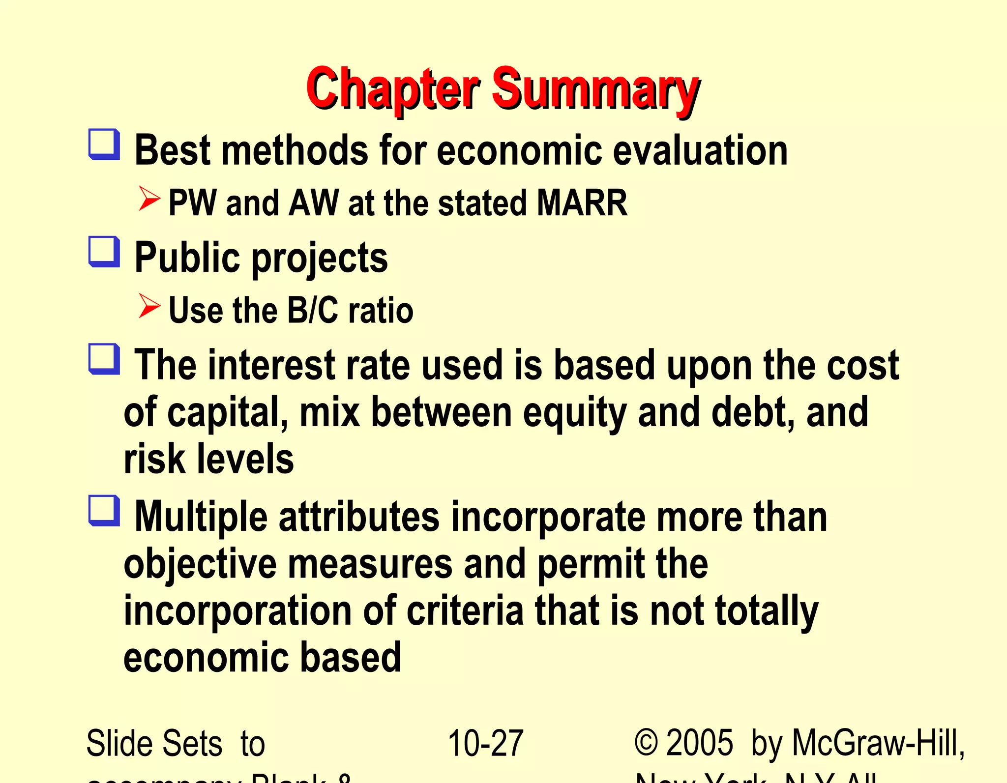
The document provides an executive summary of Chapter 10 from a textbook on engineering economy. It covers several key topics from the chapter, including different evaluation methods for comparing alternatives, determining the minimum attractive rate of return (MARR), accounting for debt and equity in the weighted average cost of capital (WACC), and methods for multi-attribute decision analysis. The summary highlights the importance of selecting the appropriate evaluation method based on problem characteristics, and calculating the MARR and WACC to evaluate investment opportunities.

1. Slide Sets to © 2005 by McGraw-Hill,10-1
Developed By:
Dr. Don Smith, P.E.
Department of Industrial
Engineering
Texas A&M University
College Station, Texas
Executive Summary Version
Chapter 10
Making Choices: The
Method, MARR, and
Multiple Attributes

2. Slide Sets to © 2005 by McGraw-Hill,10-2
LEARNING OBJECTIVESLEARNING OBJECTIVES
1. Choose a
Method
2. Cost of capital
and MARR
3. WACC –
Weighted
Average Cost of
Capital
4. Cost of debt
capital
5. Cost of equity
capital
6. High D-E mixes
7. Multiple
attributes
8. Weighted
attribute methods

3. Slide Sets to © 2005 by McGraw-Hill,10-3
Sct 10.1 Comparing Mutually ExclusiveSct 10.1 Comparing Mutually Exclusive
Alternatives by Different Evaluation MethodsAlternatives by Different Evaluation Methods
 Different problem types lend themselves to
different engineering economy methods
 Different information is available from
different evaluation methods
 Primary criteria for what method to apply
Speed
Ease of performing the analysis
 See Tables 10-1 & 10-2 for a concise summary

4. Slide Sets to © 2005 by McGraw-Hill,10-4
Evaluation TimesEvaluation Times
 Equal lives of the alternatives
PW, AW, FW
 LCM of lives
PW approach
 Specified study period
Normally exercised in industry
 Infinity (capitalized cost)

5. Slide Sets to © 2005 by McGraw-Hill,10-5
Decision GuidelinesDecision Guidelines
 Select the alternative with:
 Numerically largest
PW, FW, or AW value
For ROR and B/C
 Apply the incremental analysis approach

6. Slide Sets to © 2005 by McGraw-Hill,10-6
Sct 10.2 MARR Relative to the Cost ofSct 10.2 MARR Relative to the Cost of
CapitalCapital
 Establishing the MARR within the enterprise
 Requires:
Cost of equity capital (cost of corporate funds)
 Cost of retained earnings included here
Cost of debt capital (cost of borrowed funds)
 Debt Capital
$$ acquired from borrowing outside of the firm
 Equity Capital
$$ acquired from the owners and retained earnings

7. Slide Sets to © 2005 by McGraw-Hill,10-7
Cost of Capital and the MARRCost of Capital and the MARR
Established MARR
is the sum of:
(expressed as a % cost)
 Cost of capital +
 Expected return +
 Risk factor
 MARR will vary
from firm to firm
and from project to
project
Cost of capital
(%) CC
Min. MARR
Expected return
(%) ER
CC + x% = ER
Established MARR
Risk factor added (R%)
ER + R%

8. Slide Sets to © 2005 by McGraw-Hill,10-8
Factors Impacting the MARRFactors Impacting the MARR
 Perceived project risk
 Higher the risk – higher the MARR for that project
 Investment opportunity
 Expansion opportunity – may set a lower MARR
 Maintain flexibility
 Tax structure
 Higher tax rate – higher MARR
 Federal reserve monetary policy – interest rates
 Limited capital
 Tighter constraints on capital – higher MARR
 Market rates of other firms
 Competitors alter their MARR - the firm could follow suit

9. Slide Sets to © 2005 by McGraw-Hill,10-9
Sct 10.3 Debt-Equity Mix and WACCSct 10.3 Debt-Equity Mix and WACC
 D/E ratio (Debt to Equity mix)
 Ex.: 40-60 DE = {40% from debt, 60% from equity}
 Weighted Average Cost of Capital (WACC)
 WACC = (equity fraction)(cost of equity capital)
+ (debt fraction)(cost of debt capital)
 Both ‘costs’ are expressed as a percentage cost
 Example: WACC = 0.6(4%) + 0.6(9%) = 7.8%
 A variety of “models” exist that will approximate the
WACC for a given firm

10. Slide Sets to © 2005 by McGraw-Hill,10-10
WACC: Example 10.3WACC: Example 10.3
Source of Capital Amount ($) Cost (%)
Common Stock $5 million 13.7%
Retained
Earnings
$2 million 8.9%
Debt from bonds $3 million 7.5%
CS = 50%; RE = 20%; Bonds = 30%
WACC = (0.50)(13.7) + (0.20)(8.9) + (0.30)(7.5) = 10.88%
This firm’s MARR must be > 10.88%
Sum: $10 million

11. Slide Sets to © 2005 by McGraw-Hill,10-11
Tax ImplicationsTax Implications
(detailed in Chapter 17)(detailed in Chapter 17)
 WACC values are computed:
Before-tax basis
After-tax basis
 After-tax WACC = (Before Tax WACC)(1- Te)
 Where Te represents the effective tax rate
composed of:
o Federal rate
o State rate
o Local rate(s)

12. Slide Sets to © 2005 by McGraw-Hill,10-12
Sct 10.4 Determining Cost of Debt CapitalSct 10.4 Determining Cost of Debt Capital
 Debt financing
 Loans (borrowing)
 $ borrowed from banks
 $ borrowed from Insurance companies, etc
 Issuance of bonds (borrowing)
Interest on loans and bonds are tax deductible in the US
Bonds are sold (floated) within a bond market by investment
bankers on behalf of the firm
Subject to extensive state and federal regulations
 Interest payments from the firm to the lenders is tax
deductible – important cost consideration

13. Slide Sets to © 2005 by McGraw-Hill,10-13
Tax Savings from Debt FinancingTax Savings from Debt Financing
 The cost of financing by debt is lower than the actual
interest rate charged because of the tax deductibility
of the interest payments
 Assume Te = the effective tax rate (%)
 Tax Savings = ($ expenses)(Te)
 Net Cash Flow = {$ expenses - $ tax savings}
 NCF = expenses (1 – Te)
 See Example 10.4

14. Slide Sets to © 2005 by McGraw-Hill,10-14
Example of Tax Deductibility ImpactExample of Tax Deductibility Impact
on Cost of Debt Capitalon Cost of Debt Capital
 Assume a loan has a 10% interest rate charged to the
borrower
 The effective tax rate is 30%
 The after-tax cost of borrowing at 10% is
(0.10)(1 – 0.30) = (0.10)(0.70) = 0.07 or 7%
Observations
 Due to tax deductibility the effective cost is 7% after tax
 Higher tax rates result in lower after-tax borrowing rates

15. Slide Sets to © 2005 by McGraw-Hill,10-15
Sct 10.5 Determination of the Cost ofSct 10.5 Determination of the Cost of
Equity Capital and the MARREquity Capital and the MARR
 Sources of equity capital
1. Sale of preferred stock (PS)
2. Sale of common stock (CS)
3. Use of retained earnings (RE)
 RE = past profits retained within the firm
 This money belongs to the owners of the firm
 Sale of new stock is handled by investment
bankers and brokerage firms – highly
regulated – charge the firm for these sales

16. Slide Sets to © 2005 by McGraw-Hill,10-16
Types of StockTypes of Stock
 Preferred Stock
A form of ownership
Pays a stated dividend per share periodically
Generally a conservative type of stock
 Common Stock
A form of ownership
Carries more risk than preferred
No guarantee of dividends to be paid

17. Slide Sets to © 2005 by McGraw-Hill,10-17
Cost of Equity CapitalCost of Equity Capital
 Cost of equity capital generally applies some
form of a dividend growth model or valuation
model
Basic model
 “g” is the estimated annual increase in
returns to the shareholders
e
1
e
first-year dividend
R expected growth rate
price of the stock
DV
R =
P
g
= +
+

18. Slide Sets to © 2005 by McGraw-Hill,10-18
Capital Asset Pricing Model -- CAPMCapital Asset Pricing Model -- CAPM
 Re for equity capital is specified by
Re = risk-free return + premium above risk-free return
Re = Rf + β(Rm – Rf)
β = volatility of firm’s common stock relative to other stocks
ο β = 1 is the norm
Rm = return on stocks is a defined market portfolio as measured
by a prescribed index
Rf = quoted US Treasury Bill rate (considered a safe investment)
(Rm – Rf) = premium paid above the safe or “risk-free” rate
 See Example 10.6

19. Slide Sets to © 2005 by McGraw-Hill,10-19
Sct 10.6 Effect of Debt-Equity Mix onSct 10.6 Effect of Debt-Equity Mix on
Investment RiskInvestment Risk
 D-E mix (Review Section 10.3)
 As the proportion of debt increasesDue to t the
calculated cost of capital tends to decrease
 Tax advantage of deducting interest
 But…..leverage offered by larger percentage of debt
capital increases the risks of funding future projects
within the company
 Too much debt is a “bad thing”
 Objective – strive for a balance between debt and
equity funding

20. Slide Sets to © 2005 by McGraw-Hill,10-20
Too Much Debt…..Too Much Debt…..
 Use of larger percentages of debt capital
increases the risk that is assumed by
Investors (owners) and
Lenders
 Over time, investor confidence in the firm may
diminish and the value of the stock could well
decline
Difficult to attract new investment funds
Lenders will charge higher and higher interest
rates to hedge the risk

21. Slide Sets to © 2005 by McGraw-Hill,10-21
Sct 10.7 Multiple Attribute Analysis:Sct 10.7 Multiple Attribute Analysis:
Identification and Importance of Each AttributeIdentification and Importance of Each Attribute
 Refer back to Chapter 1 and
7-steps in Figure 10-5
 Up to now we have focused on one attribute
of a decision making problem
Economic attribute!
 Complex problems possess more than one
attribute
Multiple attribute analysis is often required
Quantitative attributes
Subjective attributes

22. Slide Sets to © 2005 by McGraw-Hill,10-22
Identification of Key AttributesIdentification of Key Attributes
 Must ID the key attributes
Comparison
Input from experts
Surveys
Group discussion
Delphi methods
 Tabulate and then agree on the critical mix of
subjective and objective attributes

23. Slide Sets to © 2005 by McGraw-Hill,10-23
Importance of Each AttributeImportance of Each Attribute
 Determine the extent of importance of each
attribute
Implies some form of weighting – wi
Given m attributes we want:
1
1.0
m
i
i
W
=
=∑
Value ratings Vi j
Tabular format of attributes
vs. alternatives
Weights for each
attribute

24. Slide Sets to © 2005 by McGraw-Hill,10-24
Weighting MethodologiesWeighting Methodologies
 Equal Weighting
 All defined attributes are assigned equal weights
 Default model
 May or may not be appropriate
 Rank Order
 m attributes are ranked in order of increasing importance (1
= least important; 2, 3, ….)
 Weighted Rank Order
 m attributes ranked in order of importance and apply:
1
i
i m
i
i
s
W
s
=
=
∑

25. Slide Sets to © 2005 by McGraw-Hill,10-25
Value Rating of AttributesValue Rating of Attributes
 Each alternative is assigned a value rating – Vij
for each attribute i
Can apply a scale of 0-100
Can apply a Likert Scale
4-5 graduations (prefer an even number of choices)e.g.
o Very Poor
o Poor
o Good
o Very good
See Table 10.4

26. Slide Sets to © 2005 by McGraw-Hill,10-26
Sct 10.8 Evaluation Measure for MultipleSct 10.8 Evaluation Measure for Multiple
AttributesAttributes
 Weighted Attribute Method
 Selection guideline
Choose the alternative with the largest Rjvalue
 Assumes increasing weights mean more important
attributes
Increasing Vij mean better performance for a given
alternative
 See Example 10.10
1
n
j i ij
j
R WV
=
= ∑

27. Slide Sets to © 2005 by McGraw-Hill,10-27
Chapter SummaryChapter Summary
 Best methods for economic evaluation
PW and AW at the stated MARR
 Public projects
Use the B/C ratio
 The interest rate used is based upon the cost
of capital, mix between equity and debt, and
risk levels
 Multiple attributes incorporate more than
objective measures and permit the
incorporation of criteria that is not totally
economic based

28. Slide Sets to © 2005 by McGraw-Hill,10-28
Chapter 10Chapter 10
End of SetEnd of Set