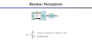
Review: Perceptron
S
x1
x2
x3
w1
w2
w3
>0? y
Properties of Perceptrons
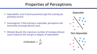
§ Separability: true if some parameters get the training set
perfectly correct
§ Convergence: if the training is separable, perceptron will
eventually converge (binary case)
§ Mistake Bound: the maximum number of mistakes (binary
case) related to the margin or degree of separability
Separable
Non-Separable
Problems with the Perceptron
§ Noise: if the data isn’t separable,
weights might thrash
§ Averaging weight vectors over time
can help (averaged perceptron)
§ Mediocre generalization: finds a
“barely” separating solution
§ Overtraining: test / held-out
accuracy usually rises, then falls
§ Overtraining is a kind of overfitting
Improving the Perceptron
Non-Separable Case: Deterministic Decision
Even the best linear boundary makes at least one mistake
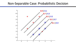
Non-Separable Case: Probabilistic Decision
0.5 | 0.5
0.3 | 0.7
0.1 | 0.9
0.7 | 0.3
0.9 | 0.1
How to get deterministic decisions?
§ Perceptron scoring:
§ If positive à classifier says: 1.0 probability this is class +1
§ If negative à classifier says: 0.0 probability this is class +1
§ Step function
§ z = output of perceptron
H(z) = probability the class is +1, according to the classifier
z = w · f(x)
z = w · f(x)
z = w · f(x)
0
1
H(z)
z
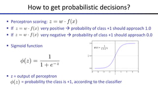
How to get probabilistic decisions?
§ Perceptron scoring:
§ If very positive à probability of class +1 should approach 1.0
§ If very negative à probability of class +1 should approach 0.0
§ Sigmoid function
§ z = output of perceptron
= probability the class is +1, according to the classifier
z = w · f(x)
z = w · f(x)
z = w · f(x)
(z) =
1
1 + e z
(z) =
1
1 + e z
Probabilistic Decisions: Example
where w is some weight constant (vector) we have to learn,
and wx is the dot product of w and x
§ Suppose w = [–3, 4, 2] and x = [1, 2, 0]
§ What label will be selected if we classify deterministically?
§ wx = –3+8+0 = 5
§ 5 is positive, so the classifier guesses the positive label
§ What are the probabilities of each label if we classify probabilistically?
§ 1 / (1 + e–5) = 0.9933 probability of positive label
§ 1 – 0.9933 = 0.0067 probability of negative label
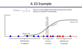
A 1D Example
definitely blue
(x negative)
definitely red
(x positive)
not sure
(x near 0)
where w is some weight constant (1D vector) we have to learn
(assume w is positive in this example)
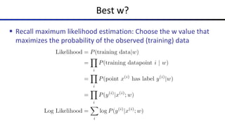
Best w?
§ Recall maximum likelihood estimation: Choose the w value that
maximizes the probability of the observed (training) data
Best w?
§ Recall maximum likelihood estimation: Choose the w value that
maximizes the probability of the observed (training) data
Best w?
§ Maximum likelihood estimation:
with:
max
w
ll(w) = max
w
X
i
log P(y(i)
|x(i)
; w)
P(y(i)
= +1|x(i)
; w) =
1
1 + e w·f(x(i))
P(y(i)
= 1|x(i)
; w) = 1
1
1 + e w·f(x(i))
= Logistic Regression
Logistic Regression Example
§ What function are we trying to maximize for this training data?
§ Data point [2, 1] is class +1
§ Data point [0, –2] is class +1
§ Data point [–1, –1] is class –1
max
w
ll(w) = max
w
X
i
log P(y(i)
|x(i)
; w)
P(y(i)
= +1|x(i)
; w) =
1
1 + e w·f(x(i))
P(y(i)
= 1|x(i)
; w) = 1
1
1 + e w·f(x(i))
+
–
+
Logistic Regression Example
§ What function are we trying to maximize for this training data?
§ Data point [2, 1] is class +1
§ Data point [0, –2] is class +1
§ Data point [–1, –1] is class –1
+
–
+
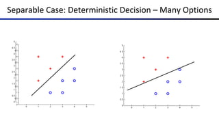
Separable Case: Deterministic Decision – Many Options
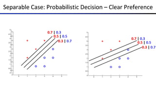
Separable Case: Probabilistic Decision – Clear Preference
0.5 | 0.5
0.3 | 0.7
0.7 | 0.3
0.5 | 0.5
0.3 | 0.7
0.7 | 0.3
Multiclass Logistic Regression
§ Recall Perceptron:
§ A weight vector for each class:
§ Score (activation) of a class y:
§ Prediction highest score wins
§ How to make the scores into probabilities?
z1, z2, z3 !
ez1
ez1 + ez2 + ez3
,
ez2
ez1 + ez2 + ez3
,
ez3
ez1 + ez2 + ez3
original activations softmax activations
Multi-Class Probabilistic Decisions: Example
§ Suppose w1 = [–3, 4, 2], w2 = [2, 2, 7], w3 = [0, –1, 0], and x = [1, 2, 0]
§ What label will be selected if we classify deterministically?
§ w1⋅x = 5, and w2⋅x = 6, and w3⋅x = –2
§ w2⋅x has the highest score, so the classifier guesses class 2
§ What are the probabilities of each label if we classify probabilistically?
§ Probability of class 1: e5 / (e5 + e6 + e–2) = 0.2689
§ Probability of class 2: e6 / (e5 + e6 + e–2) = 0.7310
§ Probability of class 3: e–2 / (e5 + e6 + e–2) = 0.0002
z1, z2, z3 !
ez1
ez1 + ez2 + ez3
,
ez2
ez1 + ez2 + ez3
,
ez3
ez1 + ez2 + ez3
Best w?
§ Recall maximum likelihood estimation: Choose the w value that
maximizes the probability of the observed (training) data
Best w?
§ Maximum likelihood estimation:
with:
max
w
ll(w) = max
w
X
i
log P(y(i)
|x(i)
; w)
P(y(i)
|x(i)
; w) =
e
wy(i) ·f(x(i)
)
P
y ewy·f(x(i))
= Multi-Class Logistic Regression
Multi-Class Logistic Regression Example
§ What function are we trying to maximize for this training data?
§ Data point [2, 1] is class Red
§ Data point [0, –2] is class Green
§ Data point [–1, –1] is class Blue
max
w
ll(w) = max
w
X
i
log P(y(i)
|x(i)
; w)
P(y(i)
|x(i)
; w) =
e
wy(i) ·f(x(i)
)
P
y ewy·f(x(i))
Multi-Class Logistic Regression Example
§ What function are we trying to maximize for this training data?
§ Data point [2, 1] is class Red
§ Data point [0, –2] is class Green
§ Data point [–1, –1] is class Blue
Log probability of [2, 1] being red
Log probability of [0,–2] being green
Log probability of [–1, –1] being blue
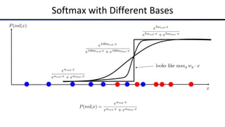
Softmax with Different Bases
Softmax and Sigmoid
§ Recall: Binary perceptron is a special case of multi-class perceptron
§ Multi-class: Compute for each class y, pick class with the highest activation
§ Binary case:
Let the weight vector of +1 be w (which we learn).
Let the weight vector of -1 always be 0 (constant).
§ Binary classification as a multi-class problem:
Activation of negative class is always 0.
If w · f is positive, then activation of +1 (w · f) is higher than -1 (0).
If w · f is negative, then activation of -1 (0) is higher than +1 (w · f).
Softmax
with wred = 0 becomes:
Sigmoid
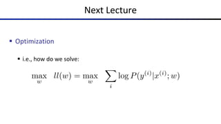
Next Lecture
§ Optimization
§ i.e., how do we solve:
max
w
ll(w) = max
w
X
i
log P(y(i)
|x(i)
; w)
Optimization and Neural Nets
Review: Derivatives and Gradients
§ What is the derivative of the function ?
§ What is the derivative of g(x) at x=5?
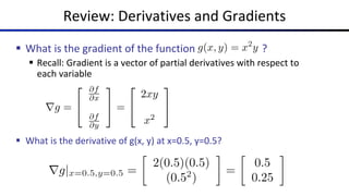
Review: Derivatives and Gradients
§ What is the gradient of the function ?
§ Recall: Gradient is a vector of partial derivatives with respect to
each variable
§ What is the derivative of g(x, y) at x=0.5, y=0.5?
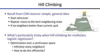
Hill Climbing
§ Recall from CSPs lecture: simple, general idea
§ Start wherever
§ Repeat: move to the best neighboring state
§ If no neighbors better than current, quit
§ What’s particularly tricky when hill-climbing for multiclass
logistic regression?
• Optimization over a continuous space
• Infinitely many neighbors!
• How to do this efficiently?
1-D Optimization
§ Could evaluate and
§ Then step in best direction
§ Or, evaluate derivative:
§ Tells which direction to step into
w
g(w)
w0
g(w0)
g(w0 + h) g(w0 h)
@g(w0)
@w
= lim
h!0
g(w0 + h) g(w0 h)
2h
2-D Optimization
Source: offconvex.org
Gradient Ascent
§ Perform update in uphill direction for each coordinate
§ The steeper the slope (i.e. the higher the derivative) the bigger the step
for that coordinate
§ E.g., consider:
§ Updates:
g(w1, w2)
w2 w2 + ↵ ⇤
@g
@w2
(w1, w2)
w1 w1 + ↵ ⇤
@g
@w1
(w1, w2)
§ Updates in vector notation:
with:
w w + ↵ ⇤ rwg(w)
rwg(w) =
"
@g
@w1
(w)
@g
@w2
(w)
#
= gradient
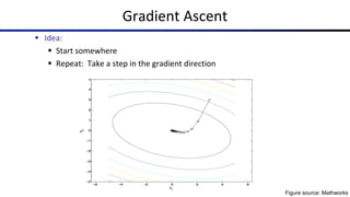
§ Idea:
§ Start somewhere
§ Repeat: Take a step in the gradient direction
Gradient Ascent
Figure source: Mathworks
What is the Steepest Direction?*
§ First-Order Taylor Expansion:
§ Steepest Descent Direction:
§ Recall: à
§ Hence, solution:
g(w + ) ⇡ g(w) +
@g
@w1
1 +
@g
@w2
2
rg =
"
@g
@w1
@g
@w2
#
Gradient direction = steepest direction!
max
: 2
1+ 2
2"
g(w + )
max
: 2
1+ 2
2"
g(w) +
@g
@w1
1 +
@g
@w2
2
= "
rg
krgk
= "
a
kak
max
:k k"
>
a
Gradient in n dimensions
rg =
2
6
6
6
4
@g
@w1
@g
@w2
· · ·
@g
@wn
3
7
7
7
5
Optimization Procedure: Gradient Ascent
§ init
§ for iter = 1, 2, …
w
§ : learning rate --- tweaking parameter that needs to be
chosen carefully
§ How? Try multiple choices
§ Crude rule of thumb: update changes about 0.1 – 1 %
↵
w
w w + ↵ ⇤ rg(w)
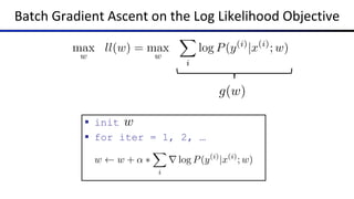
Batch Gradient Ascent on the Log Likelihood Objective
max
w
ll(w) = max
w
X
i
log P(y(i)
|x(i)
; w)
g(w)
§ init
§ for iter = 1, 2, …
w
w w + ↵ ⇤
X
i
r log P(y(i)
|x(i)
; w)
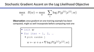
Stochastic Gradient Ascent on the Log Likelihood Objective
max
w
ll(w) = max
w
X
i
log P(y(i)
|x(i)
; w)
§ init
§ for iter = 1, 2, …
§ pick random j
w
w w + ↵ ⇤ r log P(y(j)
|x(j)
; w)
Observation: once gradient on one training example has been
computed, might as well incorporate before computing next one
Mini-Batch Gradient Ascent on the Log Likelihood Objective
max
w
ll(w) = max
w
X
i
log P(y(i)
|x(i)
; w)
§ init
§ for iter = 1, 2, …
§ pick random subset of training examples J
w
Observation: gradient over small set of training examples (=mini-batch)
can be computed in parallel, might as well do that instead of a single one
w w + ↵ ⇤
X
j2J
r log P(y(j)
|x(j)
; w)
§ We’ll talk about that once we covered neural networks, which
are a generalization of logistic regression
How about computing all the derivatives?
Neural Network Architectures
Brand new untested slides ahead – apologies for any typos/mistakes!
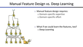
Manual Feature Design vs. Deep Learning
o Manual feature design requires:
o Domain-specific expertise
o Domain-specific effort
o What if we could learn the features, too?
o Deep Learning
Review: Perceptron
S
x1
x2
x3
w1
w2
w3
>0? y
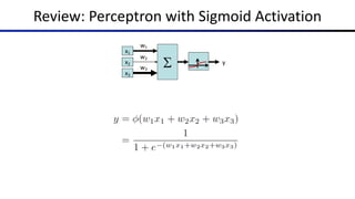
Review: Perceptron with Sigmoid Activation
S
x1
x2
x3
w1
w2
w3
y
>0?
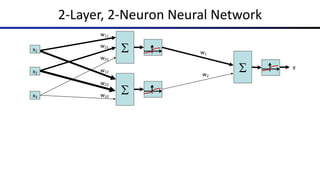
2-Layer, 2-Neuron Neural Network
x1
x2
x3
S
w12
w22
w32
>0?
S
w11
w21
w31
>0?
S
w1
w2
y
2-Layer, 2-Neuron Neural Network
x1
x2
x3
S
w12
>0?
S
w11
w21
w31
>0?
S
w1
w2
y
intermediate output h1
w22
w32
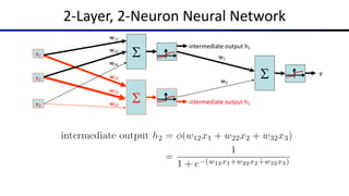
2-Layer, 2-Neuron Neural Network
x1
x2
x3
S
w12
w22
w32
>0?
S
w11
w21
w31
>0?
S
w1
w2
y
intermediate output h1
intermediate output h2
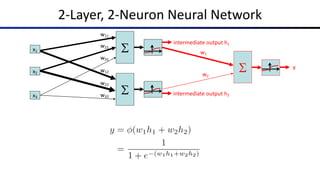
2-Layer, 2-Neuron Neural Network
x1
x2
x3
S
w12
w22
w32
>0?
S
w11
w21
w31
>0?
S
w1
w2
y
intermediate output h1
intermediate output h2
2-Layer, 2-Neuron Neural Network
x1
x2
x3
S
w12
w22
w32
>0?
S
w11
w21
w31
>0?
S
w1
w2
y
intermediate output h1
intermediate output h2
2-Layer, 2-Neuron Neural Network
The same equation, formatted with matrices:
The same equation, formatted more compactly by introducing variables representing each matrix:
2-Layer, 2-Neuron Neural Network
Shape (1, 3).
Input feature vector.
Shape (3, 2).
Weights to be learned.
Shape (1, 2).
Outputs of layer 1,
inputs to layer 2.
Shape (1, 2).
Outputs of layer 1,
inputs to layer 2.
Shape (2, 1).
Weights to be learned.
Shape (1, 1).
Output of network.
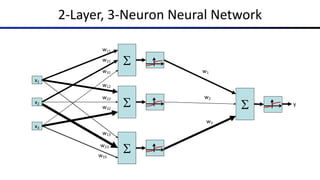
2-Layer, 3-Neuron Neural Network
S
x1
x2
x3
w13
w23
w33
>0?
S
w12
w22
w32
>0?
S
w11
w21
w31
>0?
S
w1
w2
w3
y
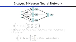
2-Layer, 3-Neuron Neural Network
Shape (1, 3).
Input feature vector.
Shape (3, 3).
Weights to be learned
Shape (1, 3).
Outputs of layer 1,
inputs to layer 2.
Shape (1, 3).
Outputs of layer 1,
inputs to layer 2.
Shape (3, 1).
Weights to be learned.
Shape (1, 1).
Output of network.
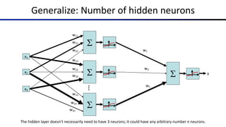
Generalize: Number of hidden neurons
S
x1
x2
x3
w1n
w2n
w3n
>0?
S
w12
w22
w32
>0?
S
w11
w21
w31
>0?
S
w1
w2
wn
y
…
The hidden layer doesn’t necessarily need to have 3 neurons; it could have any arbitrary number n neurons.
Generalize: Number of hidden neurons
Shape (1, 3).
Input feature vector.
Shape (3, n).
Weights to be learned
Shape (1, n).
Outputs of layer 1,
inputs to layer 2.
Shape (1, n).
Outputs of layer 1,
inputs to layer 2.
Shape (n, 1).
Weights to be learned.
Shape (1, 1).
Output of network.
The hidden layer doesn’t necessarily need to have 3 neurons; it could have any arbitrary number n neurons.
Generalize: Number of input features
S
x1
x2
x3
w1n
w2n
w3n
>0?
wdim(x)1
S
w11
w21
w31
>0?
S
w1
wn
y
…
…
xdim(x)
wdim(x)n
The input feature vector doesn’t necessarily need to have 3 features; it could have some arbitrary number dim(x) of features.
Generalize: Number of input features
Shape (1, dim(x)).
Input feature vector.
Shape (dim(x), n).
Weights to be learned
Shape (1, n).
Outputs of layer 1,
inputs to layer 2.
Shape (1, n).
Outputs of layer 1,
inputs to layer 2.
Shape (n, 1).
Weights to be learned.
Shape (1, 1).
Output of network.
The input feature vector doesn’t necessarily need to have 3 features; it could have some arbitrary number dim(x) of features.
Generalize: Number of outputs
S
x1
x2
x3
w1n
w2n
w3n
>0?
Wdim(x)1
S
w11
w21
w31
>0?
S y1
…
…
xdim(x)
wdim(x)n
S ydim(y)
…
The output doesn’t necessarily need to be just one number; it could be some arbitrary dim(y) length vector.
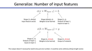
Generalize: Number of input features
Shape (1, dim(x)).
Input feature vector.
Shape (dim(x), n).
Weights to be learned
Shape (1, n).
Outputs of layer 1,
inputs to layer 2.
Shape (1, n).
Outputs of layer 1,
inputs to layer 2.
Shape (n, dim(y)).
Weights to be learned.
Shape (1, dim(y)).
Output of network.
The output doesn’t necessarily need to be just one number; it could be some arbitrary dim(y) length vector.
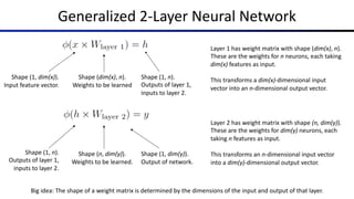
Generalized 2-Layer Neural Network
Shape (1, dim(x)).
Input feature vector.
Shape (dim(x), n).
Weights to be learned
Shape (1, n).
Outputs of layer 1,
inputs to layer 2.
Shape (1, n).
Outputs of layer 1,
inputs to layer 2.
Shape (n, dim(y)).
Weights to be learned.
Shape (1, dim(y)).
Output of network.
Big idea: The shape of a weight matrix is determined by the dimensions of the input and output of that layer.
Layer 1 has weight matrix with shape (dim(x), n).
These are the weights for n neurons, each taking
dim(x) features as input.
This transforms a dim(x)-dimensional input
vector into an n-dimensional output vector.
Layer 2 has weight matrix with shape (n, dim(y)).
These are the weights for dim(y) neurons, each
taking n features as input.
This transforms an n-dimensional input vector
into a dim(y)-dimensional output vector.
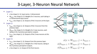
3-Layer, 3-Neuron Neural Network
S
x1
x2
x3
>0?
S >0?
S >0?
S >0?
S >0?
S >0?
S y
3-Layer, 3-Neuron Neural Network
§ Layer 1:
§ x has shape (1, 3). Input vector, 3-dimensional.
§ Wlayer 1 has shape (3, 3). Weights for 3 neurons, each taking in
a 3-dimensional input vector.
§ hlayer 1 has shape (1, 3). Outputs of the 3 neurons at this layer.
§ Layer 2:
§ hlayer 1 has shape (1, 3). Outputs of the 3 neurons from the
previous layer.
§ Wlayer 2 has shape (3, 3). Weights for 3 new neurons, each
taking in the 3 previous perceptron outputs.
§ hlayer 2 has shape (1, 3). Outputs of the 3 new neurons at this
layer.
§ Layer 3:
§ hlayer 2 has shape (1, 3). Outputs from the previous layer.
§ Wlayer 3 has shape (3, 1). Weights for 1 final neuron, taking in
the 3 previous perceptron outputs.
§ y has shape (1, 1). Output of the final neuron.
Generalized 3-Layer Neural Network
§ Layer 1:
§ x has shape (1, dim(x))
§ Wlayer 1 has shape (dim(x), dim(L1))
§ hlayer 1 has shape (1, dim(L1))
§ Layer 2:
§ hlayer 1 has shape (1, dim(L1))
§ Wlayer 2 has shape (dim(L1), dim(L2))
§ hlayer 2 has shape (1, dim(L2))
§ Layer 3:
§ hlayer 2 has shape (1, dim(L2))
§ Wlayer 3 has shape (dim(L2), dim(y))
§ y has shape (1, dim(y))
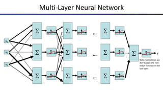
Multi-Layer Neural Network
S
x1
x2
x3
>0?
S >0?
S >0?
S
S >0?
S >0?
S >0?
S >0?
S >0?
S >0?
…
…
…
y
Note: Sometimes we
don’t apply the non-
linear function in the
last layer.
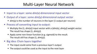
Multi-Layer Neural Network
§ Input to a layer: some dim(x)-dimensional input vector
§ Output of a layer: some dim(y)-dimensional output vector
§ dim(y) is the number of neurons in the layer (1 output per neuron)
§ Process of converting input to output:
§ Multiply the (1, dim(x)) input vector with a (dim(x), dim(y)) weight vector.
The result has shape (1, dim(y)).
§ Apply some non-linear function (e.g. sigmoid) to the result.
The result still has shape (1, dim(y)).
§ Big idea: Chain layers together
§ The input could come from a previous layer’s output
§ The output could be used as the input to the next layer
Deep Neural Network
…
x1
x2
x3
xL
… … … …
z
(1)
1
z
(1)
2
z
(1)
3
z
(1)
K(1) z
(n)
K(n)
z
(2)
K(2)
z
(2)
1
z
(2)
2
z
(2)
3 z
(n)
3
z
(n)
2
z
(n)
1
z
(OUT )
1
z
(OUT )
2
z
(OUT )
3
z
(n 1)
3
z
(n 1)
2
z
(n 1)
1
z
(n 1)
K(n 1)
…
z
(k)
i = g(
X
j
W
(k 1,k)
i,j z
(k 1)
j ) g = nonlinear activation function
Common Activation Functions
[source: MIT 6.S191 introtodeeplearning.com]
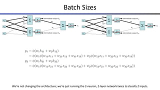
Batch Sizes
x11
x21
x31
S
w12
w22
w32
>0?
S
w11
w21
w31
>0?
S
w1
w2
y1
intermediate output h11
intermediate output h21
x12
x22
x32
S
w12
w22
w32
>0?
S
w11
w21
w31
>0?
S
w1
w2
y2
intermediate output h12
intermediate output h22
Batch Sizes
We’re not changing the architecture; we’re just running the 2-neuron, 2-layer network twice to classify 2 inputs.
Batch Sizes
Rewriting in matrix form:
Batch Sizes
Shape (batch, dim(x)).
Input feature vector.
Shape (dim(x), n).
Weights to be learned
Shape (batch, n).
Outputs of layer 1,
inputs to layer 2.
Shape (batch, n).
Outputs of layer 1,
inputs to layer 2.
Shape (n, dim(y)).
Weights to be learned.
Shape (batch, dim(y)).
Output of network.
Big idea: We can “stack” inputs together to classify multiple inputs at once. The result is multiple outputs “stacked” together.
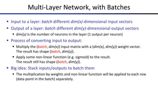
Multi-Layer Network, with Batches
§ Input to a layer: batch different dim(x)-dimensional input vectors
§ Output of a layer: batch different dim(y)-dimensional output vectors
§ dim(y) is the number of neurons in the layer (1 output per neuron)
§ Process of converting input to output:
§ Multiply the (batch, dim(x)) input matrix with a (dim(x), dim(y)) weight vector.
The result has shape (batch, dim(y)).
§ Apply some non-linear function (e.g. sigmoid) to the result.
The result still has shape (batch, dim(y)).
§ Big idea: Stack inputs/outputs to batch them
§ The multiplication by weights and non-linear function will be applied to each row
(data point in the batch) separately.
Training Neural Networks
§ Step 1: For each input in the training (sub)set x, predict a classification y
using the current weights
§ Step 2: Compare predictions with the true y values, using a loss function
§ Higher value of loss function = bad model
§ Lower value of loss function = good model
§ Example: zero-one loss: count the number of misclassified inputs
§ Example: log loss (derived from maximum likelihood; more on this soon)
§ Example: sum of squared errors (if you’re solving a regression problem)
§ Step 3: Use numerical method (e.g. gradient descent) to minimize loss
§ Loss is a function of the weights. Optimization goal: find weights that minimize loss
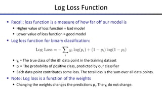
Log Loss Function
§ Recall: loss function is a measure of how far off our model is
§ Higher value of loss function = bad model
§ Lower value of loss function = good model
§ Log loss function for binary classification:
§ yi = The true class of the ith data point in the training dataset
§ pi = The probability of positive class, predicted by our classifier
§ Each data point contributes some loss. The total loss is the sum over all data points.
§ Note: Log loss is a function of the weights
§ Changing the weights changes the predictions pi. The yi do not change.
Log Loss Function
§ Log loss function for a single data point:
§ Case I: True class is y = 1
§ Log loss function becomes just –log(p)
§ If classifier gives p near 0:
The model was confident in guessing y=0
Bad model à high loss value
§ If classifier gives p near 1:
The model was confident in guessing y=1
Good model à low loss value
Log Loss Function
§ Log loss function for a single data point:
§ Case II: True class is y = 0
§ Log loss function becomes just –log(1-p)
§ If classifier gives p near 0:
The model was confident in guessing y=0
Good model à low loss value
§ If classifier gives p near 1:
The model was confident in guessing y=1
Bad model à high loss value
§ Note: This equation uses y=0, not y=-1,
for the negative class
Log Loss Example
§ Data point 1: True class y=1. We predicted p=0.1 probability it’s the positive class.
§ Intuitively: Our guess is bad. We should have guessed closer to p=1.
§ This contributes –log(0.1) = 1 to the loss function.
§ Data point 2: True class y=0. We predicted p=0 probability it’s the positive class.
§ Intuitively: Our guess was perfect. We were certain it was y=0.
§ This contributes –log(1.0) = 0 to our loss function.
§ Data point 3: True class y=1. We predicted 0.8 probability it’s the positive class.
§ Intuitively: Our guess was pretty good, but not perfect.
§ This contributes –log(0.8) = 0.1 to the loss function.
§ Total loss: 1 + 0 + 0.1 = 1.1
§ Goal: Find the weights that lead to the probabilities that minimize this loss function
Optimization Procedure: Gradient Descent
§ init
§ for iter = 1, 2, …
where
and is computed by running the network on input xi and weights w
w
§ : learning rate --- tweaking parameter that needs to be
chosen carefully
↵
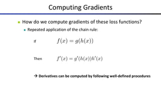
Computing Gradients
n How do we compute gradients of these loss functions?
n Repeated application of the chain rule:
If
Then
à Derivatives can be computed by following well-defined procedures
f(x) = g(h(x))
f0
(x) = g0
(h(x))h0
(x)
§ Automatic differentiation software
§ e.g. Theano, TensorFlow, PyTorch, Chainer
§ Only need to program the function g(x,y,w)
§ Can automatically compute all derivatives w.r.t. all entries in w
§ This is typically done by caching info during forward computation pass
of f, and then doing a backward pass = “backpropagation”
§ Autodiff / Backpropagation can often be done at computational cost
comparable to the forward pass
§ Need to know this exists
§ How this is done? -- outside of scope of CS188
Automatic Differentiation
§ Gradient of at w1 = 2, w2 = 3, w3 = 2
§ Think of g as a composition of many functions
§ Then, we can use the chain rule to compute the gradient
§ g = b + c
§ b = a × w2
§ a = w1
4
§ c = 5w1
Backpropagation*
w1
w2
w3
^4
×
×
+
5
w1 = 2
w2 = 3
w3 = 2
a = 16
b = 48
c = 10
g = 58
Properties of Neural Networks
Neural Networks Properties
§ Theorem (Universal Function Approximators). A two-layer neural
network with a sufficient number of neurons can approximate
any continuous function to any desired accuracy.
§ Practical considerations
§ Can be seen as learning the features
§ Large number of neurons
§ Danger for overfitting
§ (hence early stopping!)
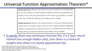
Universal Function Approximation Theorem*
§ In words: Given any continuous function f(x), if a 2-layer neural
network has enough hidden units, then there is a choice of
weights that allow it to closely approximate f(x).
Cybenko (1989) “Approximations by superpositions of sigmoidal functions”
Hornik (1991) “Approximation Capabilities of Multilayer Feedforward Networks”
Leshno and Schocken (1991) ”Multilayer Feedforward Networks with Non-Polynomial Activation
Functions Can Approximate Any Function”
Universal Function Approximation Theorem*
Cybenko (1989) “Approximations by superpositions of sigmoidal functions”
Hornik (1991) “Approximation Capabilities of Multilayer Feedforward Networks”
Leshno and Schocken (1991) ”Multilayer Feedforward Networks with Non-Polynomial Activation
Functions Can Approximate Any Function”
Summary of Key Ideas
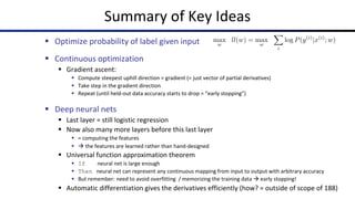
§ Optimize probability of label given input
§ Continuous optimization
§ Gradient ascent:
§ Compute steepest uphill direction = gradient (= just vector of partial derivatives)
§ Take step in the gradient direction
§ Repeat (until held-out data accuracy starts to drop = “early stopping”)
§ Deep neural nets
§ Last layer = still logistic regression
§ Now also many more layers before this last layer
§ = computing the features
§ à the features are learned rather than hand-designed
§ Universal function approximation theorem
§ If neural net is large enough
§ Then neural net can represent any continuous mapping from input to output with arbitrary accuracy
§ But remember: need to avoid overfitting / memorizing the training data à early stopping!
§ Automatic differentiation gives the derivatives efficiently (how? = outside of scope of 188)
max
w
ll(w) = max
w
X
i
log P(y(i)
|x(i)
; w)
Application: Computer Vision
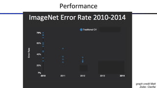
Performance
graph credit Matt
Zeiler, Clarifai
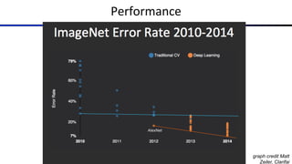
Performance
graph credit Matt
Zeiler, Clarifai
Performance
graph credit Matt
Zeiler, Clarifai
AlexNet
Performance
graph credit Matt
Zeiler, Clarifai
AlexNet
Performance
graph credit Matt
Zeiler, Clarifai
AlexNet
Fun Neural Net Demo Site
§ Demo-site:
§ http://playground.tensorflow.org/
Next: More Neural Net Applications!

Review : Perceptron Artificial Intelligence.pdf

  • 1.
  • 2.
    Properties of Perceptrons §Separability: true if some parameters get the training set perfectly correct § Convergence: if the training is separable, perceptron will eventually converge (binary case) § Mistake Bound: the maximum number of mistakes (binary case) related to the margin or degree of separability Separable Non-Separable
  • 3.
    Problems with thePerceptron § Noise: if the data isn’t separable, weights might thrash § Averaging weight vectors over time can help (averaged perceptron) § Mediocre generalization: finds a “barely” separating solution § Overtraining: test / held-out accuracy usually rises, then falls § Overtraining is a kind of overfitting
  • 4.
  • 5.
    Non-Separable Case: DeterministicDecision Even the best linear boundary makes at least one mistake
  • 6.
    Non-Separable Case: ProbabilisticDecision 0.5 | 0.5 0.3 | 0.7 0.1 | 0.9 0.7 | 0.3 0.9 | 0.1
  • 7.
    How to getdeterministic decisions? § Perceptron scoring: § If positive à classifier says: 1.0 probability this is class +1 § If negative à classifier says: 0.0 probability this is class +1 § Step function § z = output of perceptron H(z) = probability the class is +1, according to the classifier z = w · f(x) z = w · f(x) z = w · f(x) 0 1 H(z) z
  • 8.
    How to getprobabilistic decisions? § Perceptron scoring: § If very positive à probability of class +1 should approach 1.0 § If very negative à probability of class +1 should approach 0.0 § Sigmoid function § z = output of perceptron = probability the class is +1, according to the classifier z = w · f(x) z = w · f(x) z = w · f(x) (z) = 1 1 + e z (z) = 1 1 + e z
  • 9.
    Probabilistic Decisions: Example wherew is some weight constant (vector) we have to learn, and wx is the dot product of w and x § Suppose w = [–3, 4, 2] and x = [1, 2, 0] § What label will be selected if we classify deterministically? § wx = –3+8+0 = 5 § 5 is positive, so the classifier guesses the positive label § What are the probabilities of each label if we classify probabilistically? § 1 / (1 + e–5) = 0.9933 probability of positive label § 1 – 0.9933 = 0.0067 probability of negative label
  • 10.
    A 1D Example definitelyblue (x negative) definitely red (x positive) not sure (x near 0) where w is some weight constant (1D vector) we have to learn (assume w is positive in this example)
  • 11.
    Best w? § Recallmaximum likelihood estimation: Choose the w value that maximizes the probability of the observed (training) data
  • 12.
    Best w? § Recallmaximum likelihood estimation: Choose the w value that maximizes the probability of the observed (training) data
  • 13.
    Best w? § Maximumlikelihood estimation: with: max w ll(w) = max w X i log P(y(i) |x(i) ; w) P(y(i) = +1|x(i) ; w) = 1 1 + e w·f(x(i)) P(y(i) = 1|x(i) ; w) = 1 1 1 + e w·f(x(i)) = Logistic Regression
  • 14.
    Logistic Regression Example §What function are we trying to maximize for this training data? § Data point [2, 1] is class +1 § Data point [0, –2] is class +1 § Data point [–1, –1] is class –1 max w ll(w) = max w X i log P(y(i) |x(i) ; w) P(y(i) = +1|x(i) ; w) = 1 1 + e w·f(x(i)) P(y(i) = 1|x(i) ; w) = 1 1 1 + e w·f(x(i)) + – +
  • 15.
    Logistic Regression Example §What function are we trying to maximize for this training data? § Data point [2, 1] is class +1 § Data point [0, –2] is class +1 § Data point [–1, –1] is class –1 + – +
  • 16.
    Separable Case: DeterministicDecision – Many Options
  • 17.
    Separable Case: ProbabilisticDecision – Clear Preference 0.5 | 0.5 0.3 | 0.7 0.7 | 0.3 0.5 | 0.5 0.3 | 0.7 0.7 | 0.3
  • 18.
    Multiclass Logistic Regression §Recall Perceptron: § A weight vector for each class: § Score (activation) of a class y: § Prediction highest score wins § How to make the scores into probabilities? z1, z2, z3 ! ez1 ez1 + ez2 + ez3 , ez2 ez1 + ez2 + ez3 , ez3 ez1 + ez2 + ez3 original activations softmax activations
  • 19.
    Multi-Class Probabilistic Decisions:Example § Suppose w1 = [–3, 4, 2], w2 = [2, 2, 7], w3 = [0, –1, 0], and x = [1, 2, 0] § What label will be selected if we classify deterministically? § w1⋅x = 5, and w2⋅x = 6, and w3⋅x = –2 § w2⋅x has the highest score, so the classifier guesses class 2 § What are the probabilities of each label if we classify probabilistically? § Probability of class 1: e5 / (e5 + e6 + e–2) = 0.2689 § Probability of class 2: e6 / (e5 + e6 + e–2) = 0.7310 § Probability of class 3: e–2 / (e5 + e6 + e–2) = 0.0002 z1, z2, z3 ! ez1 ez1 + ez2 + ez3 , ez2 ez1 + ez2 + ez3 , ez3 ez1 + ez2 + ez3
  • 20.
    Best w? § Recallmaximum likelihood estimation: Choose the w value that maximizes the probability of the observed (training) data
  • 21.
    Best w? § Maximumlikelihood estimation: with: max w ll(w) = max w X i log P(y(i) |x(i) ; w) P(y(i) |x(i) ; w) = e wy(i) ·f(x(i) ) P y ewy·f(x(i)) = Multi-Class Logistic Regression
  • 22.
    Multi-Class Logistic RegressionExample § What function are we trying to maximize for this training data? § Data point [2, 1] is class Red § Data point [0, –2] is class Green § Data point [–1, –1] is class Blue max w ll(w) = max w X i log P(y(i) |x(i) ; w) P(y(i) |x(i) ; w) = e wy(i) ·f(x(i) ) P y ewy·f(x(i))
  • 23.
    Multi-Class Logistic RegressionExample § What function are we trying to maximize for this training data? § Data point [2, 1] is class Red § Data point [0, –2] is class Green § Data point [–1, –1] is class Blue Log probability of [2, 1] being red Log probability of [0,–2] being green Log probability of [–1, –1] being blue
  • 24.
  • 25.
    Softmax and Sigmoid §Recall: Binary perceptron is a special case of multi-class perceptron § Multi-class: Compute for each class y, pick class with the highest activation § Binary case: Let the weight vector of +1 be w (which we learn). Let the weight vector of -1 always be 0 (constant). § Binary classification as a multi-class problem: Activation of negative class is always 0. If w · f is positive, then activation of +1 (w · f) is higher than -1 (0). If w · f is negative, then activation of -1 (0) is higher than +1 (w · f). Softmax with wred = 0 becomes: Sigmoid
  • 26.
    Next Lecture § Optimization §i.e., how do we solve: max w ll(w) = max w X i log P(y(i) |x(i) ; w)
  • 27.
  • 28.
    Review: Derivatives andGradients § What is the derivative of the function ? § What is the derivative of g(x) at x=5?
  • 29.
    Review: Derivatives andGradients § What is the gradient of the function ? § Recall: Gradient is a vector of partial derivatives with respect to each variable § What is the derivative of g(x, y) at x=0.5, y=0.5?
  • 30.
    Hill Climbing § Recallfrom CSPs lecture: simple, general idea § Start wherever § Repeat: move to the best neighboring state § If no neighbors better than current, quit § What’s particularly tricky when hill-climbing for multiclass logistic regression? • Optimization over a continuous space • Infinitely many neighbors! • How to do this efficiently?
  • 31.
    1-D Optimization § Couldevaluate and § Then step in best direction § Or, evaluate derivative: § Tells which direction to step into w g(w) w0 g(w0) g(w0 + h) g(w0 h) @g(w0) @w = lim h!0 g(w0 + h) g(w0 h) 2h
  • 32.
  • 33.
    Gradient Ascent § Performupdate in uphill direction for each coordinate § The steeper the slope (i.e. the higher the derivative) the bigger the step for that coordinate § E.g., consider: § Updates: g(w1, w2) w2 w2 + ↵ ⇤ @g @w2 (w1, w2) w1 w1 + ↵ ⇤ @g @w1 (w1, w2) § Updates in vector notation: with: w w + ↵ ⇤ rwg(w) rwg(w) = " @g @w1 (w) @g @w2 (w) # = gradient
  • 34.
    § Idea: § Startsomewhere § Repeat: Take a step in the gradient direction Gradient Ascent Figure source: Mathworks
  • 35.
    What is theSteepest Direction?* § First-Order Taylor Expansion: § Steepest Descent Direction: § Recall: à § Hence, solution: g(w + ) ⇡ g(w) + @g @w1 1 + @g @w2 2 rg = " @g @w1 @g @w2 # Gradient direction = steepest direction! max : 2 1+ 2 2" g(w + ) max : 2 1+ 2 2" g(w) + @g @w1 1 + @g @w2 2 = " rg krgk = " a kak max :k k" > a
  • 36.
    Gradient in ndimensions rg = 2 6 6 6 4 @g @w1 @g @w2 · · · @g @wn 3 7 7 7 5
  • 37.
    Optimization Procedure: GradientAscent § init § for iter = 1, 2, … w § : learning rate --- tweaking parameter that needs to be chosen carefully § How? Try multiple choices § Crude rule of thumb: update changes about 0.1 – 1 % ↵ w w w + ↵ ⇤ rg(w)
  • 38.
    Batch Gradient Ascenton the Log Likelihood Objective max w ll(w) = max w X i log P(y(i) |x(i) ; w) g(w) § init § for iter = 1, 2, … w w w + ↵ ⇤ X i r log P(y(i) |x(i) ; w)
  • 39.
    Stochastic Gradient Ascenton the Log Likelihood Objective max w ll(w) = max w X i log P(y(i) |x(i) ; w) § init § for iter = 1, 2, … § pick random j w w w + ↵ ⇤ r log P(y(j) |x(j) ; w) Observation: once gradient on one training example has been computed, might as well incorporate before computing next one
  • 40.
    Mini-Batch Gradient Ascenton the Log Likelihood Objective max w ll(w) = max w X i log P(y(i) |x(i) ; w) § init § for iter = 1, 2, … § pick random subset of training examples J w Observation: gradient over small set of training examples (=mini-batch) can be computed in parallel, might as well do that instead of a single one w w + ↵ ⇤ X j2J r log P(y(j) |x(j) ; w)
  • 41.
    § We’ll talkabout that once we covered neural networks, which are a generalization of logistic regression How about computing all the derivatives?
  • 42.
    Neural Network Architectures Brandnew untested slides ahead – apologies for any typos/mistakes!
  • 43.
    Manual Feature Designvs. Deep Learning o Manual feature design requires: o Domain-specific expertise o Domain-specific effort o What if we could learn the features, too? o Deep Learning
  • 44.
  • 45.
    Review: Perceptron withSigmoid Activation S x1 x2 x3 w1 w2 w3 y >0?
  • 46.
    2-Layer, 2-Neuron NeuralNetwork x1 x2 x3 S w12 w22 w32 >0? S w11 w21 w31 >0? S w1 w2 y
  • 47.
    2-Layer, 2-Neuron NeuralNetwork x1 x2 x3 S w12 >0? S w11 w21 w31 >0? S w1 w2 y intermediate output h1 w22 w32
  • 48.
    2-Layer, 2-Neuron NeuralNetwork x1 x2 x3 S w12 w22 w32 >0? S w11 w21 w31 >0? S w1 w2 y intermediate output h1 intermediate output h2
  • 49.
    2-Layer, 2-Neuron NeuralNetwork x1 x2 x3 S w12 w22 w32 >0? S w11 w21 w31 >0? S w1 w2 y intermediate output h1 intermediate output h2
  • 50.
    2-Layer, 2-Neuron NeuralNetwork x1 x2 x3 S w12 w22 w32 >0? S w11 w21 w31 >0? S w1 w2 y intermediate output h1 intermediate output h2
  • 51.
    2-Layer, 2-Neuron NeuralNetwork The same equation, formatted with matrices: The same equation, formatted more compactly by introducing variables representing each matrix:
  • 52.
    2-Layer, 2-Neuron NeuralNetwork Shape (1, 3). Input feature vector. Shape (3, 2). Weights to be learned. Shape (1, 2). Outputs of layer 1, inputs to layer 2. Shape (1, 2). Outputs of layer 1, inputs to layer 2. Shape (2, 1). Weights to be learned. Shape (1, 1). Output of network.
  • 53.
    2-Layer, 3-Neuron NeuralNetwork S x1 x2 x3 w13 w23 w33 >0? S w12 w22 w32 >0? S w11 w21 w31 >0? S w1 w2 w3 y
  • 54.
  • 55.
    2-Layer, 3-Neuron NeuralNetwork Shape (1, 3). Input feature vector. Shape (3, 3). Weights to be learned Shape (1, 3). Outputs of layer 1, inputs to layer 2. Shape (1, 3). Outputs of layer 1, inputs to layer 2. Shape (3, 1). Weights to be learned. Shape (1, 1). Output of network.
  • 56.
    Generalize: Number ofhidden neurons S x1 x2 x3 w1n w2n w3n >0? S w12 w22 w32 >0? S w11 w21 w31 >0? S w1 w2 wn y … The hidden layer doesn’t necessarily need to have 3 neurons; it could have any arbitrary number n neurons.
  • 57.
    Generalize: Number ofhidden neurons Shape (1, 3). Input feature vector. Shape (3, n). Weights to be learned Shape (1, n). Outputs of layer 1, inputs to layer 2. Shape (1, n). Outputs of layer 1, inputs to layer 2. Shape (n, 1). Weights to be learned. Shape (1, 1). Output of network. The hidden layer doesn’t necessarily need to have 3 neurons; it could have any arbitrary number n neurons.
  • 58.
    Generalize: Number ofinput features S x1 x2 x3 w1n w2n w3n >0? wdim(x)1 S w11 w21 w31 >0? S w1 wn y … … xdim(x) wdim(x)n The input feature vector doesn’t necessarily need to have 3 features; it could have some arbitrary number dim(x) of features.
  • 59.
    Generalize: Number ofinput features Shape (1, dim(x)). Input feature vector. Shape (dim(x), n). Weights to be learned Shape (1, n). Outputs of layer 1, inputs to layer 2. Shape (1, n). Outputs of layer 1, inputs to layer 2. Shape (n, 1). Weights to be learned. Shape (1, 1). Output of network. The input feature vector doesn’t necessarily need to have 3 features; it could have some arbitrary number dim(x) of features.
  • 60.
    Generalize: Number ofoutputs S x1 x2 x3 w1n w2n w3n >0? Wdim(x)1 S w11 w21 w31 >0? S y1 … … xdim(x) wdim(x)n S ydim(y) … The output doesn’t necessarily need to be just one number; it could be some arbitrary dim(y) length vector.
  • 61.
    Generalize: Number ofinput features Shape (1, dim(x)). Input feature vector. Shape (dim(x), n). Weights to be learned Shape (1, n). Outputs of layer 1, inputs to layer 2. Shape (1, n). Outputs of layer 1, inputs to layer 2. Shape (n, dim(y)). Weights to be learned. Shape (1, dim(y)). Output of network. The output doesn’t necessarily need to be just one number; it could be some arbitrary dim(y) length vector.
  • 62.
    Generalized 2-Layer NeuralNetwork Shape (1, dim(x)). Input feature vector. Shape (dim(x), n). Weights to be learned Shape (1, n). Outputs of layer 1, inputs to layer 2. Shape (1, n). Outputs of layer 1, inputs to layer 2. Shape (n, dim(y)). Weights to be learned. Shape (1, dim(y)). Output of network. Big idea: The shape of a weight matrix is determined by the dimensions of the input and output of that layer. Layer 1 has weight matrix with shape (dim(x), n). These are the weights for n neurons, each taking dim(x) features as input. This transforms a dim(x)-dimensional input vector into an n-dimensional output vector. Layer 2 has weight matrix with shape (n, dim(y)). These are the weights for dim(y) neurons, each taking n features as input. This transforms an n-dimensional input vector into a dim(y)-dimensional output vector.
  • 63.
    3-Layer, 3-Neuron NeuralNetwork S x1 x2 x3 >0? S >0? S >0? S >0? S >0? S >0? S y
  • 64.
    3-Layer, 3-Neuron NeuralNetwork § Layer 1: § x has shape (1, 3). Input vector, 3-dimensional. § Wlayer 1 has shape (3, 3). Weights for 3 neurons, each taking in a 3-dimensional input vector. § hlayer 1 has shape (1, 3). Outputs of the 3 neurons at this layer. § Layer 2: § hlayer 1 has shape (1, 3). Outputs of the 3 neurons from the previous layer. § Wlayer 2 has shape (3, 3). Weights for 3 new neurons, each taking in the 3 previous perceptron outputs. § hlayer 2 has shape (1, 3). Outputs of the 3 new neurons at this layer. § Layer 3: § hlayer 2 has shape (1, 3). Outputs from the previous layer. § Wlayer 3 has shape (3, 1). Weights for 1 final neuron, taking in the 3 previous perceptron outputs. § y has shape (1, 1). Output of the final neuron.
  • 65.
    Generalized 3-Layer NeuralNetwork § Layer 1: § x has shape (1, dim(x)) § Wlayer 1 has shape (dim(x), dim(L1)) § hlayer 1 has shape (1, dim(L1)) § Layer 2: § hlayer 1 has shape (1, dim(L1)) § Wlayer 2 has shape (dim(L1), dim(L2)) § hlayer 2 has shape (1, dim(L2)) § Layer 3: § hlayer 2 has shape (1, dim(L2)) § Wlayer 3 has shape (dim(L2), dim(y)) § y has shape (1, dim(y))
  • 66.
    Multi-Layer Neural Network S x1 x2 x3 >0? S>0? S >0? S S >0? S >0? S >0? S >0? S >0? S >0? … … … y Note: Sometimes we don’t apply the non- linear function in the last layer.
  • 67.
    Multi-Layer Neural Network §Input to a layer: some dim(x)-dimensional input vector § Output of a layer: some dim(y)-dimensional output vector § dim(y) is the number of neurons in the layer (1 output per neuron) § Process of converting input to output: § Multiply the (1, dim(x)) input vector with a (dim(x), dim(y)) weight vector. The result has shape (1, dim(y)). § Apply some non-linear function (e.g. sigmoid) to the result. The result still has shape (1, dim(y)). § Big idea: Chain layers together § The input could come from a previous layer’s output § The output could be used as the input to the next layer
  • 68.
    Deep Neural Network … x1 x2 x3 xL …… … … z (1) 1 z (1) 2 z (1) 3 z (1) K(1) z (n) K(n) z (2) K(2) z (2) 1 z (2) 2 z (2) 3 z (n) 3 z (n) 2 z (n) 1 z (OUT ) 1 z (OUT ) 2 z (OUT ) 3 z (n 1) 3 z (n 1) 2 z (n 1) 1 z (n 1) K(n 1) … z (k) i = g( X j W (k 1,k) i,j z (k 1) j ) g = nonlinear activation function
  • 69.
    Common Activation Functions [source:MIT 6.S191 introtodeeplearning.com]
  • 70.
    Batch Sizes x11 x21 x31 S w12 w22 w32 >0? S w11 w21 w31 >0? S w1 w2 y1 intermediate outputh11 intermediate output h21 x12 x22 x32 S w12 w22 w32 >0? S w11 w21 w31 >0? S w1 w2 y2 intermediate output h12 intermediate output h22
  • 71.
    Batch Sizes We’re notchanging the architecture; we’re just running the 2-neuron, 2-layer network twice to classify 2 inputs.
  • 72.
  • 73.
    Batch Sizes Shape (batch,dim(x)). Input feature vector. Shape (dim(x), n). Weights to be learned Shape (batch, n). Outputs of layer 1, inputs to layer 2. Shape (batch, n). Outputs of layer 1, inputs to layer 2. Shape (n, dim(y)). Weights to be learned. Shape (batch, dim(y)). Output of network. Big idea: We can “stack” inputs together to classify multiple inputs at once. The result is multiple outputs “stacked” together.
  • 74.
    Multi-Layer Network, withBatches § Input to a layer: batch different dim(x)-dimensional input vectors § Output of a layer: batch different dim(y)-dimensional output vectors § dim(y) is the number of neurons in the layer (1 output per neuron) § Process of converting input to output: § Multiply the (batch, dim(x)) input matrix with a (dim(x), dim(y)) weight vector. The result has shape (batch, dim(y)). § Apply some non-linear function (e.g. sigmoid) to the result. The result still has shape (batch, dim(y)). § Big idea: Stack inputs/outputs to batch them § The multiplication by weights and non-linear function will be applied to each row (data point in the batch) separately.
  • 75.
  • 76.
    Training Neural Networks §Step 1: For each input in the training (sub)set x, predict a classification y using the current weights § Step 2: Compare predictions with the true y values, using a loss function § Higher value of loss function = bad model § Lower value of loss function = good model § Example: zero-one loss: count the number of misclassified inputs § Example: log loss (derived from maximum likelihood; more on this soon) § Example: sum of squared errors (if you’re solving a regression problem) § Step 3: Use numerical method (e.g. gradient descent) to minimize loss § Loss is a function of the weights. Optimization goal: find weights that minimize loss
  • 77.
    Log Loss Function §Recall: loss function is a measure of how far off our model is § Higher value of loss function = bad model § Lower value of loss function = good model § Log loss function for binary classification: § yi = The true class of the ith data point in the training dataset § pi = The probability of positive class, predicted by our classifier § Each data point contributes some loss. The total loss is the sum over all data points. § Note: Log loss is a function of the weights § Changing the weights changes the predictions pi. The yi do not change.
  • 78.
    Log Loss Function §Log loss function for a single data point: § Case I: True class is y = 1 § Log loss function becomes just –log(p) § If classifier gives p near 0: The model was confident in guessing y=0 Bad model à high loss value § If classifier gives p near 1: The model was confident in guessing y=1 Good model à low loss value
  • 79.
    Log Loss Function §Log loss function for a single data point: § Case II: True class is y = 0 § Log loss function becomes just –log(1-p) § If classifier gives p near 0: The model was confident in guessing y=0 Good model à low loss value § If classifier gives p near 1: The model was confident in guessing y=1 Bad model à high loss value § Note: This equation uses y=0, not y=-1, for the negative class
  • 80.
    Log Loss Example §Data point 1: True class y=1. We predicted p=0.1 probability it’s the positive class. § Intuitively: Our guess is bad. We should have guessed closer to p=1. § This contributes –log(0.1) = 1 to the loss function. § Data point 2: True class y=0. We predicted p=0 probability it’s the positive class. § Intuitively: Our guess was perfect. We were certain it was y=0. § This contributes –log(1.0) = 0 to our loss function. § Data point 3: True class y=1. We predicted 0.8 probability it’s the positive class. § Intuitively: Our guess was pretty good, but not perfect. § This contributes –log(0.8) = 0.1 to the loss function. § Total loss: 1 + 0 + 0.1 = 1.1 § Goal: Find the weights that lead to the probabilities that minimize this loss function
  • 81.
    Optimization Procedure: GradientDescent § init § for iter = 1, 2, … where and is computed by running the network on input xi and weights w w § : learning rate --- tweaking parameter that needs to be chosen carefully ↵
  • 82.
    Computing Gradients n Howdo we compute gradients of these loss functions? n Repeated application of the chain rule: If Then à Derivatives can be computed by following well-defined procedures f(x) = g(h(x)) f0 (x) = g0 (h(x))h0 (x)
  • 83.
    § Automatic differentiationsoftware § e.g. Theano, TensorFlow, PyTorch, Chainer § Only need to program the function g(x,y,w) § Can automatically compute all derivatives w.r.t. all entries in w § This is typically done by caching info during forward computation pass of f, and then doing a backward pass = “backpropagation” § Autodiff / Backpropagation can often be done at computational cost comparable to the forward pass § Need to know this exists § How this is done? -- outside of scope of CS188 Automatic Differentiation
  • 84.
    § Gradient ofat w1 = 2, w2 = 3, w3 = 2 § Think of g as a composition of many functions § Then, we can use the chain rule to compute the gradient § g = b + c § b = a × w2 § a = w1 4 § c = 5w1 Backpropagation* w1 w2 w3 ^4 × × + 5 w1 = 2 w2 = 3 w3 = 2 a = 16 b = 48 c = 10 g = 58
  • 85.
  • 86.
    Neural Networks Properties §Theorem (Universal Function Approximators). A two-layer neural network with a sufficient number of neurons can approximate any continuous function to any desired accuracy. § Practical considerations § Can be seen as learning the features § Large number of neurons § Danger for overfitting § (hence early stopping!)
  • 87.
    Universal Function ApproximationTheorem* § In words: Given any continuous function f(x), if a 2-layer neural network has enough hidden units, then there is a choice of weights that allow it to closely approximate f(x). Cybenko (1989) “Approximations by superpositions of sigmoidal functions” Hornik (1991) “Approximation Capabilities of Multilayer Feedforward Networks” Leshno and Schocken (1991) ”Multilayer Feedforward Networks with Non-Polynomial Activation Functions Can Approximate Any Function”
  • 88.
    Universal Function ApproximationTheorem* Cybenko (1989) “Approximations by superpositions of sigmoidal functions” Hornik (1991) “Approximation Capabilities of Multilayer Feedforward Networks” Leshno and Schocken (1991) ”Multilayer Feedforward Networks with Non-Polynomial Activation Functions Can Approximate Any Function”
  • 89.
    Summary of KeyIdeas § Optimize probability of label given input § Continuous optimization § Gradient ascent: § Compute steepest uphill direction = gradient (= just vector of partial derivatives) § Take step in the gradient direction § Repeat (until held-out data accuracy starts to drop = “early stopping”) § Deep neural nets § Last layer = still logistic regression § Now also many more layers before this last layer § = computing the features § à the features are learned rather than hand-designed § Universal function approximation theorem § If neural net is large enough § Then neural net can represent any continuous mapping from input to output with arbitrary accuracy § But remember: need to avoid overfitting / memorizing the training data à early stopping! § Automatic differentiation gives the derivatives efficiently (how? = outside of scope of 188) max w ll(w) = max w X i log P(y(i) |x(i) ; w)
  • 90.
  • 91.
  • 92.
  • 93.
  • 94.
  • 95.
  • 96.
    Fun Neural NetDemo Site § Demo-site: § http://playground.tensorflow.org/
  • 97.
    Next: More NeuralNet Applications!