Application of differential calculus

1. Lecture 12
Application of differential
calculus to investigation of
behaviour of functions
Monotonicity

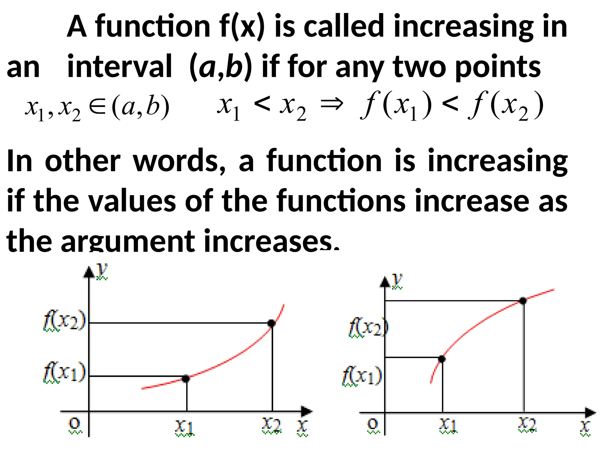
2. A function f(x) is called increasing in
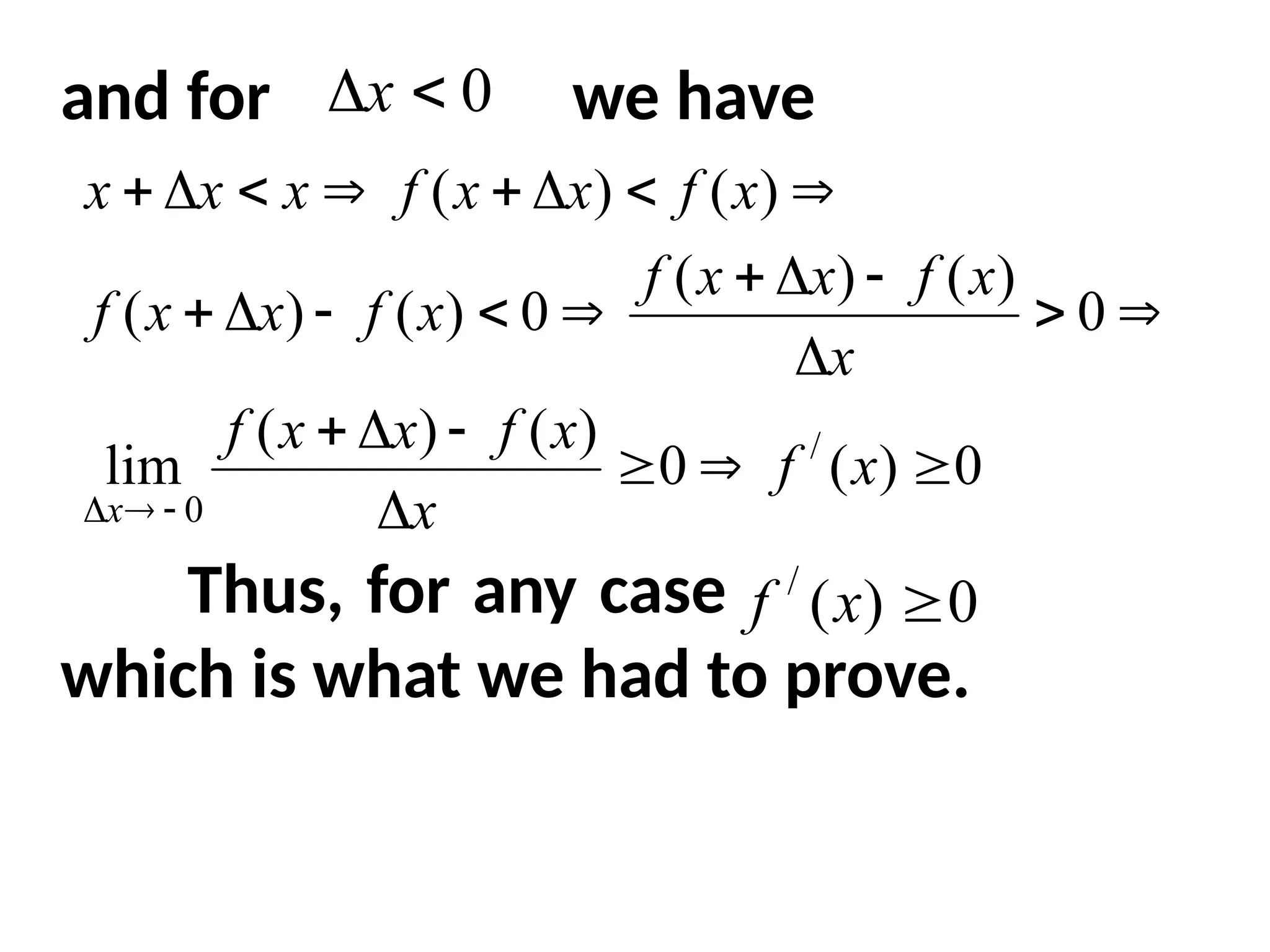
an interval (a,b) if for any two points
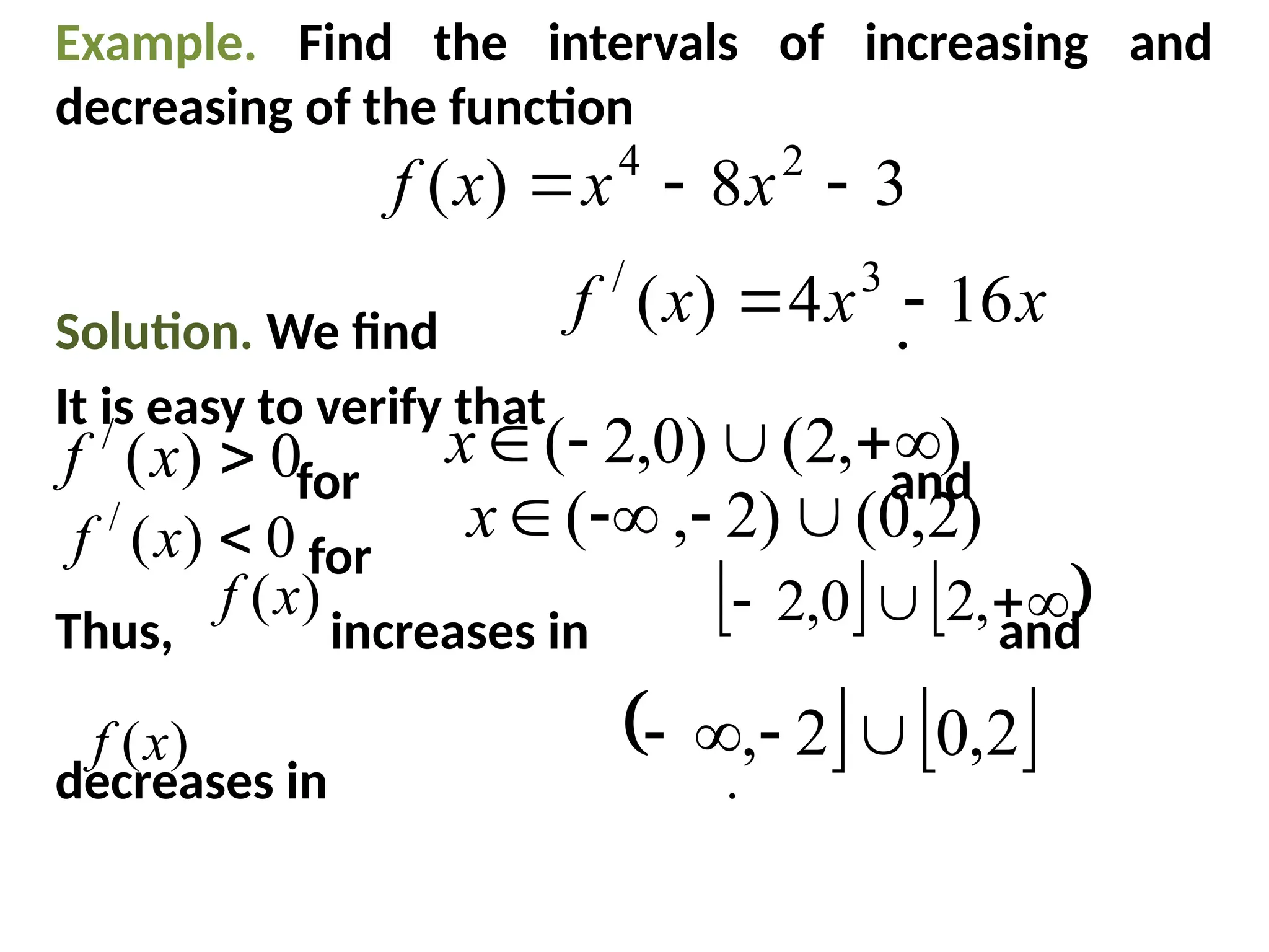
In other words, a function is increasing
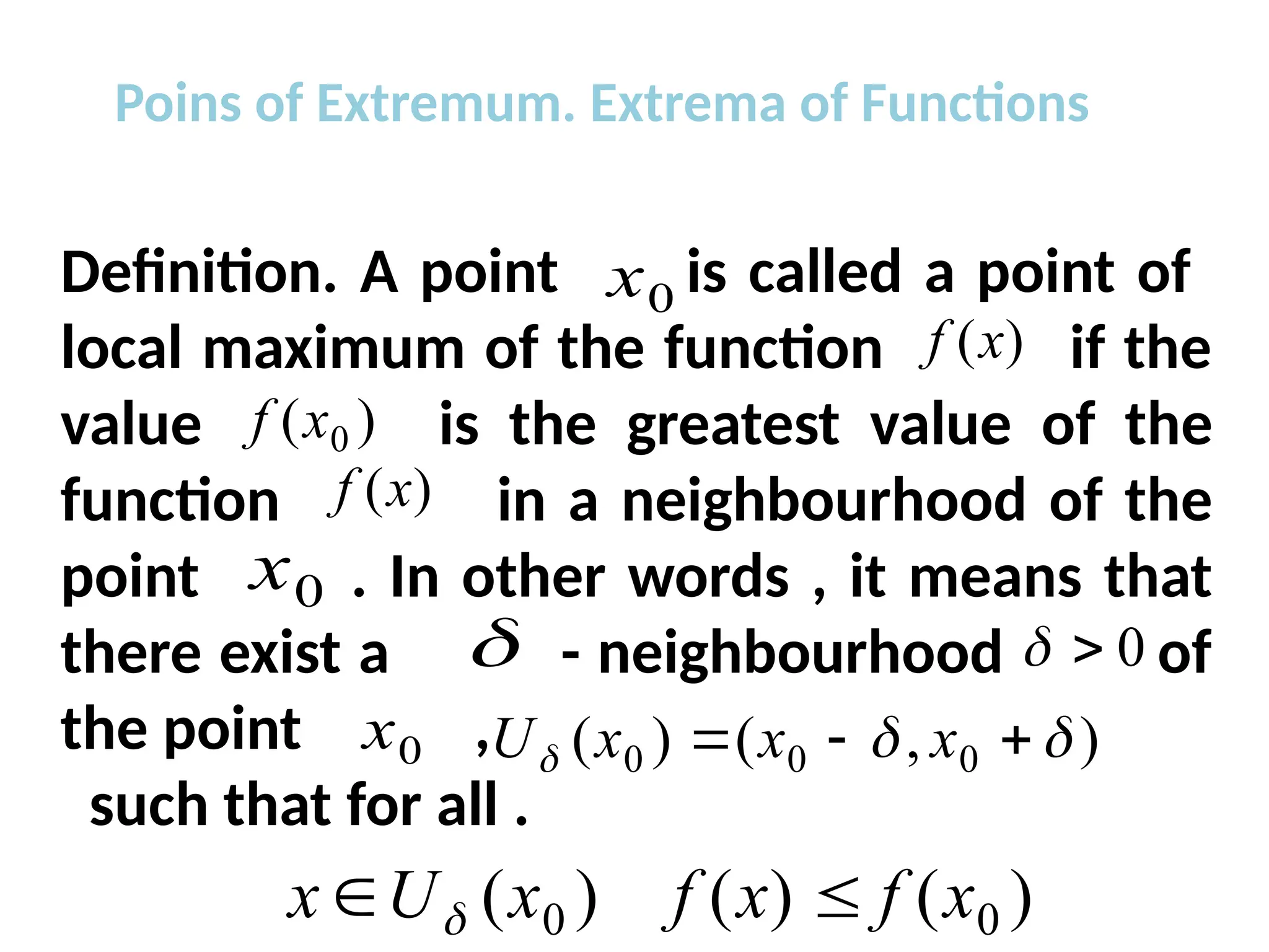
if the values of the functions increase as
the argument increases.
)
,
(
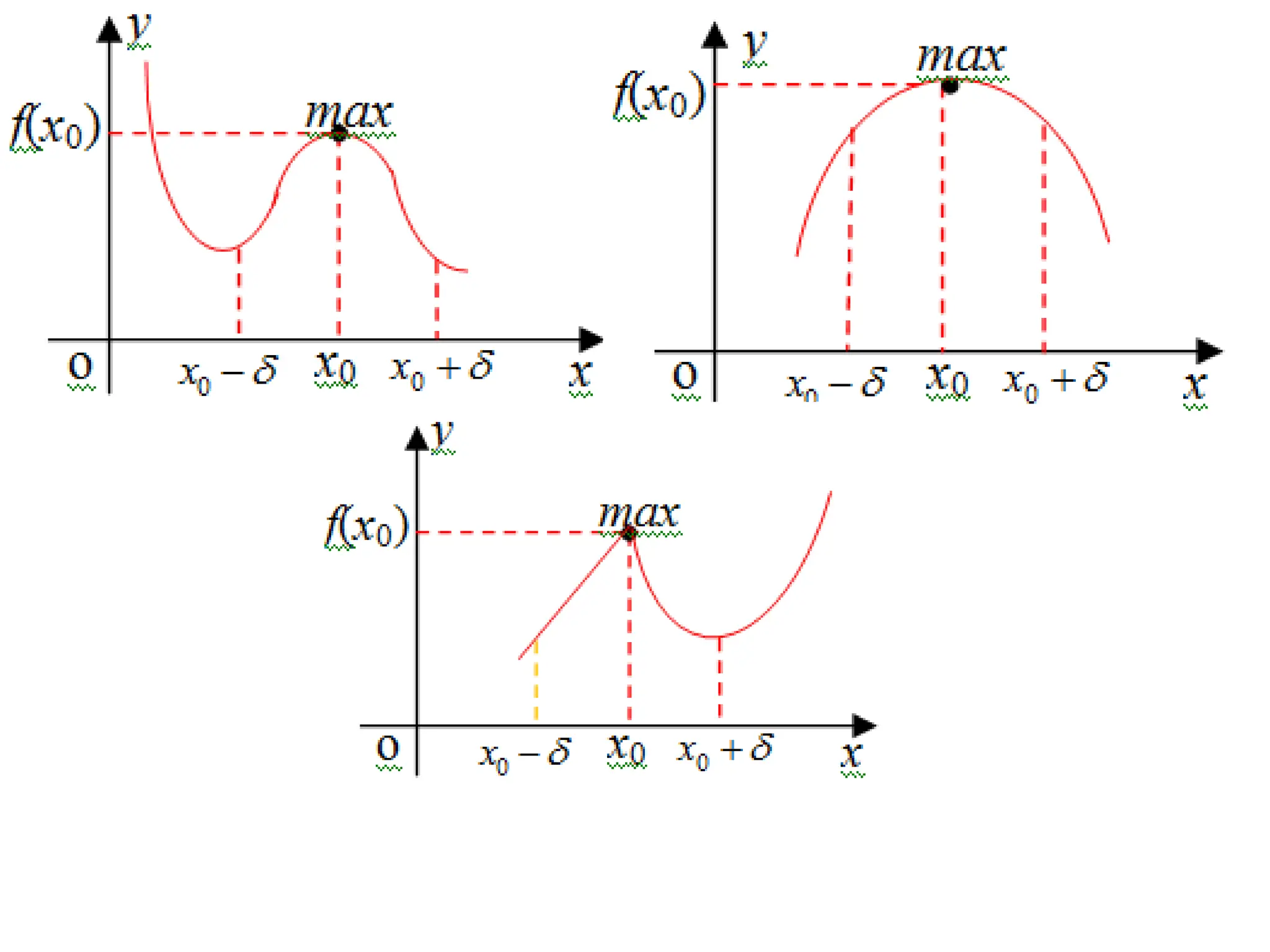
, 2
1 b
a
x
x  )
(
)
( 2
1
2
1 x
f
x
f
x
x 



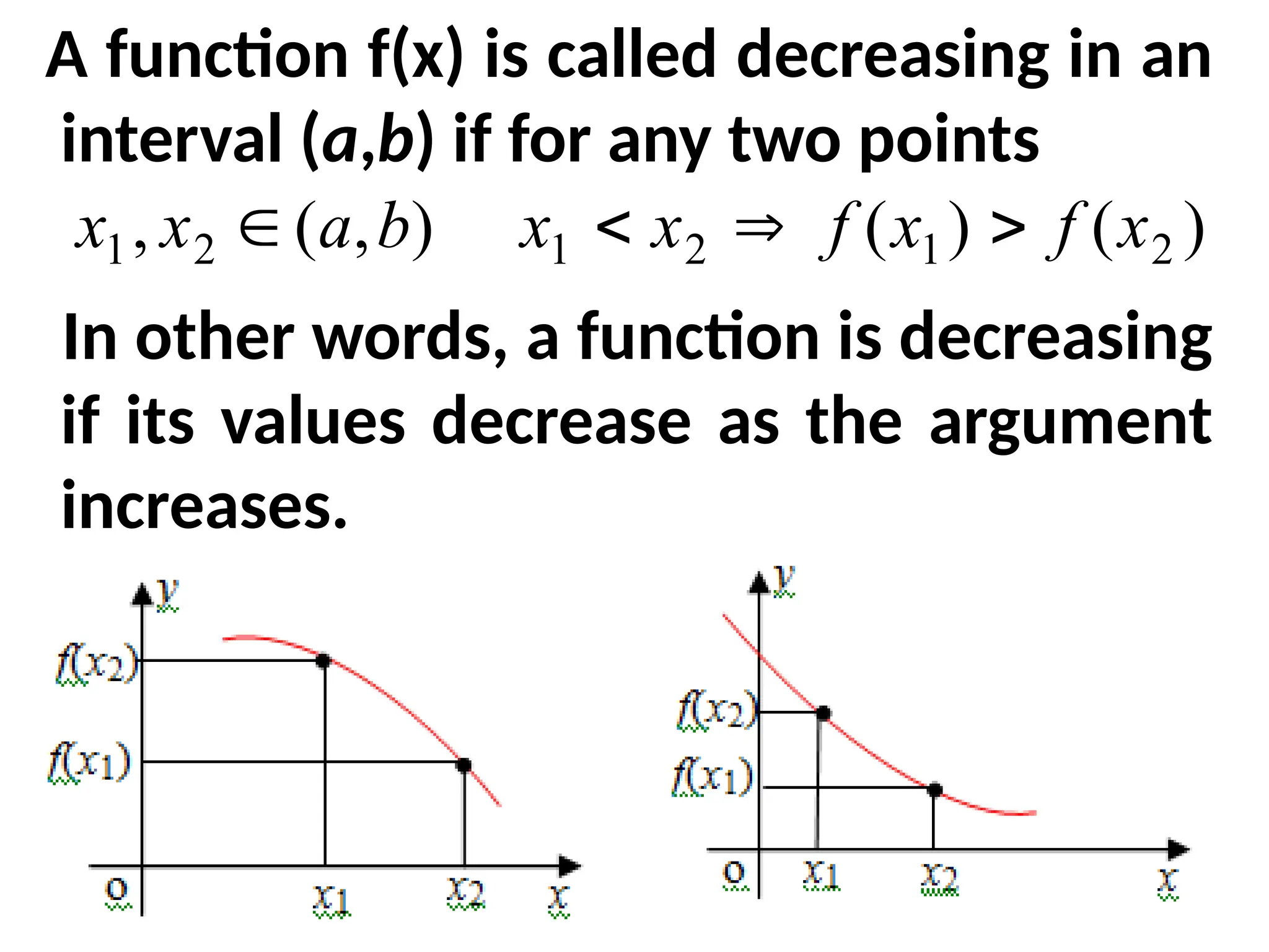
3. A function f(x) is called decreasing in an
interval (a,b) if for any two points
In other words, a function is decreasing
if its values decrease as the argument
increases.
)
,
(
, 2
1 b
a
x
x  )
(
)
( 2
1
2
1 x
f
x
f
x
x 



4. Both increasing and decreasing
functions are called monotonic.
Conditions for Monotonicity
Between the character (nature) of the
monotonicity of differentiable function and
the sigh of its derivative there is a
connection stated in the following theorem.

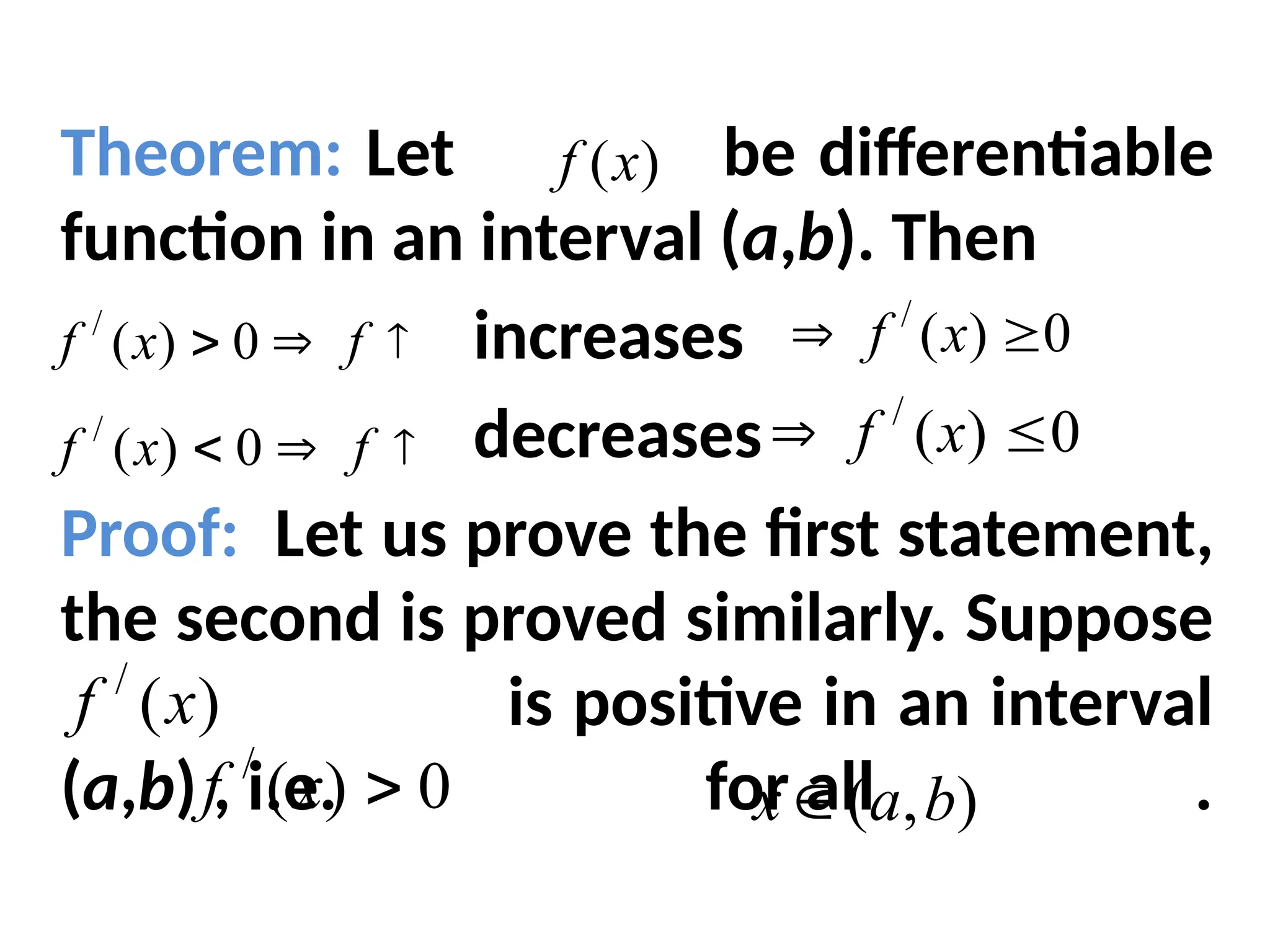
5. Theorem: Let be differentiable
function in an interval (a,b). Then
increases
decreases
Proof: Let us prove the first statement,
the second is proved similarly. Suppose
is positive in an interval
(a,b) , i.e. for all .
)
(x
f


 f
x
f 0
)
(
/ 0
)
(
/

 x
f


 f
x
f 0
)
(
/ 0
)
(
/

 x
f
)
(
/
x
f
0
)
(
/

x
f )
,
( b
a
x 

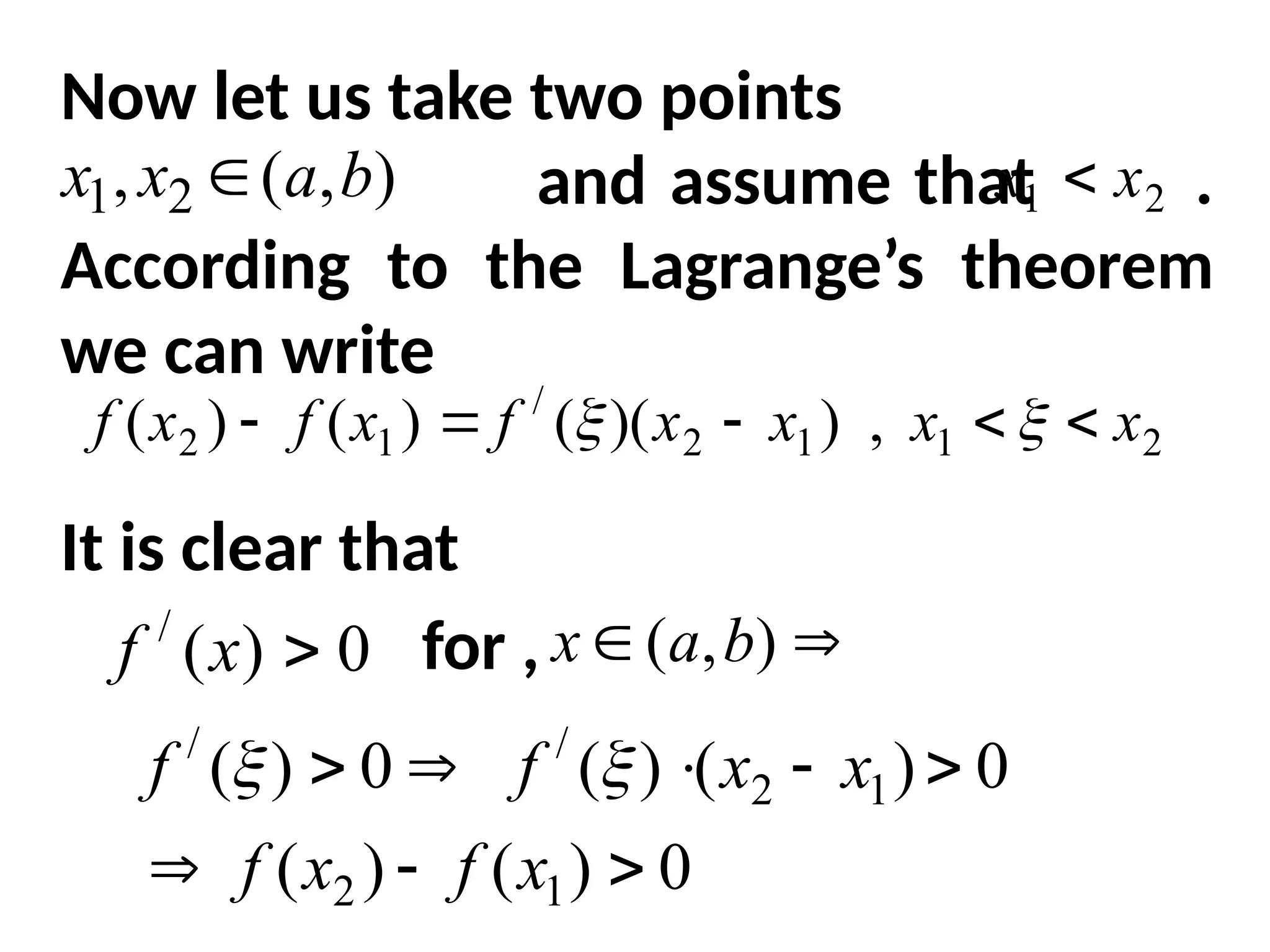
6. Now let us take two points
and assume that .
According to the Lagrange’s theorem
we can write
It is clear that
for ,
)
,
(
, 2
1 b
a
x
x  2
1 x
x 
,
)
)(
(
)
(
)
( 1
2
/
1
2 x
x
f
x
f
x
f 

  2
1 x
x 

0
)
(
/

x
f 
 )
,
( b
a
x
0
)
(
)
(
0
)
(
)
(
0
)
(
1
2
1
2
/
/








x
f
x
f
x
x
f
f 


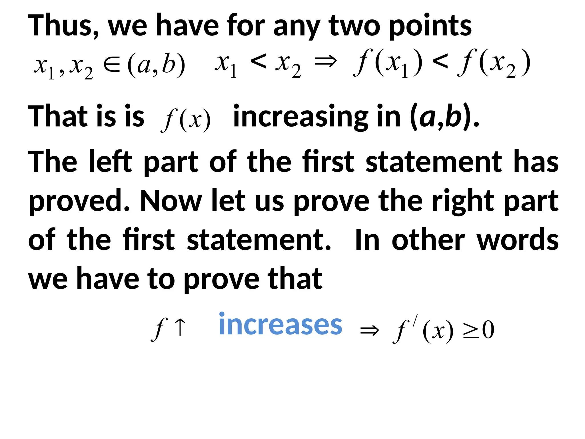
7. Thus, we have for any two points
That is is increasing in (a,b).
The left part of the first statement has
proved. Now let us prove the right part
of the first statement. In other words
we have to prove that
increases
)
,
(
, 2
1 b
a
x
x  )
(
)
( 2
1
2
1 x
f
x
f
x
x 


)
(x
f

f 0
)
(
/

 x
f

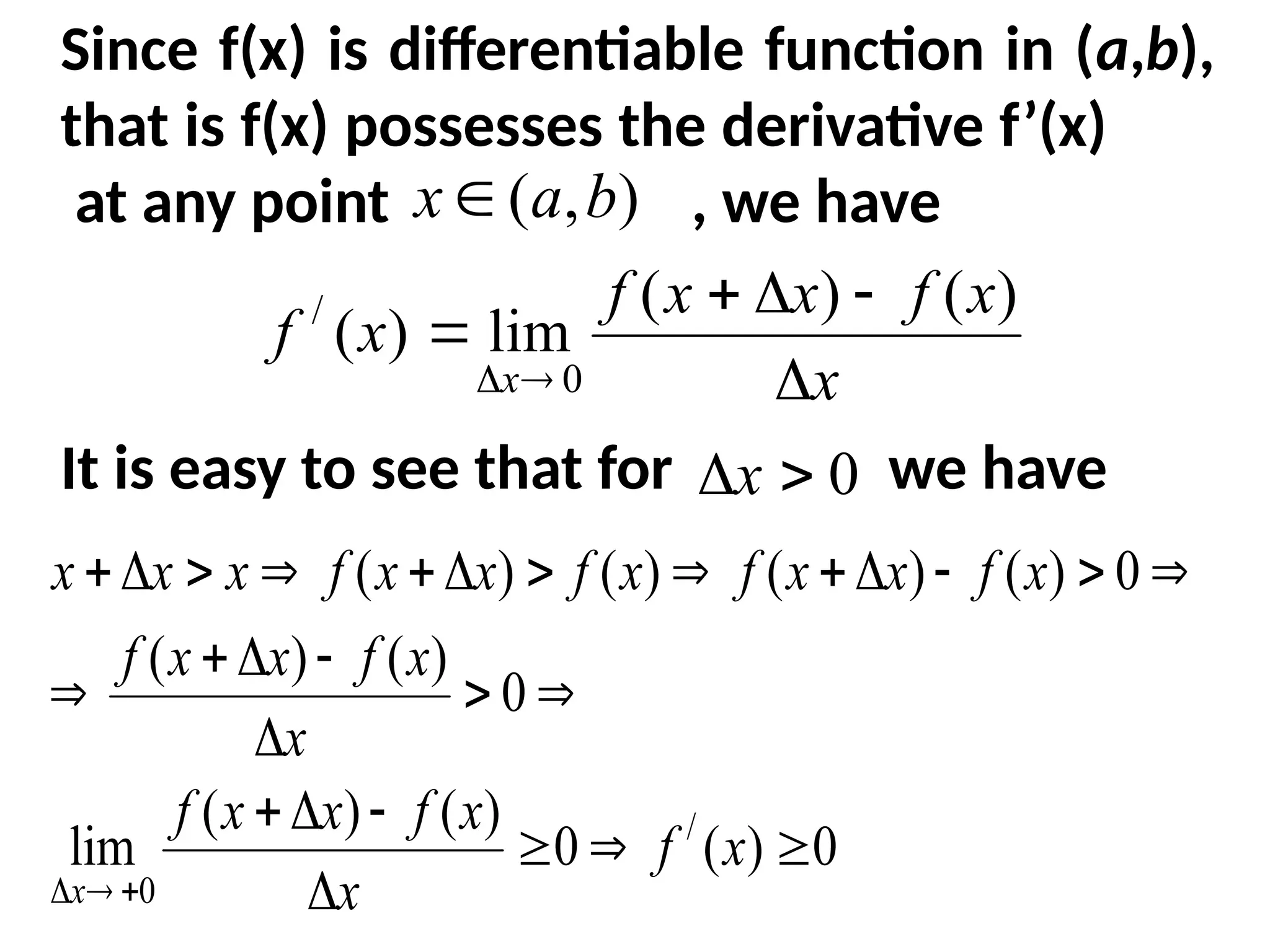
8. Since f(x) is differentiable function in (a,b),
that is f(x) possesses the derivative f’(x)
at any point , we have
It is easy to see that for we have
)
,
( b
a
x 
x
x
f
x
x
f
x
f
x 






)
(
)
(
lim
)
(
0
/
0

x
0
)
(
0
)
(
)
(
lim
0
)
(
)
(
0
)
(
)
(
)
(
)
(
/
0






























x
f
x
x
f
x
x
f
x
x
f
x
x
f
x
f
x
x
f
x
f
x
x
f
x
x
x
x

9. and for we have
Thus, for any case
which is what we had to prove.
0
)
(
0
)
(
)
(
lim
0
)
(
)
(
0
)
(
)
(
)
(
)
(
/
0





























x
f
x
x
f
x
x
f
x
x
f
x
x
f
x
f
x
x
f
x
f
x
x
f
x
x
x
x
0

x
0
)
(
/

x
f

10. Example. Find the intervals of increasing and
decreasing of the function
Solution. We find .
It is easy to verify that
for and
for
Thus, increases in and
decreases in .
3
8
)
( 2
4


 x
x
x
f
x
x
x
f 16
4
)
( 3
/


0
)
(
/

x
f )
,
2
(
)
0
,
2
( 



x
0
)
(
/

x
f )
2
,
0
(
)
2
,
( 



x
)
(x
f    


 ,
2
0
,
2
)
(x
f    
2
,
0
2
, 




11. Poins of Extremum. Extrema of Functions
Definition. A point is called a point of
local maximum of the function if the
value is the greatest value of the
function in a neighbourhood of the
point . In other words , it means that
there exist a - neighbourhood of
the point ,
such that for all .
0
x
)
(x
f
)
( 0
x
f
)
(x
f
0
x
 0


0
x )
,
(
)
( 0
0
0 

 

 x
x
x
U
)
(
)
(
)
( 0
0 x
f
x
f
x
U
x 
 

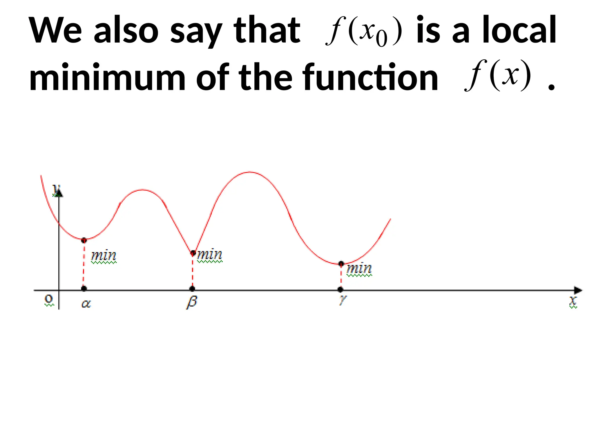
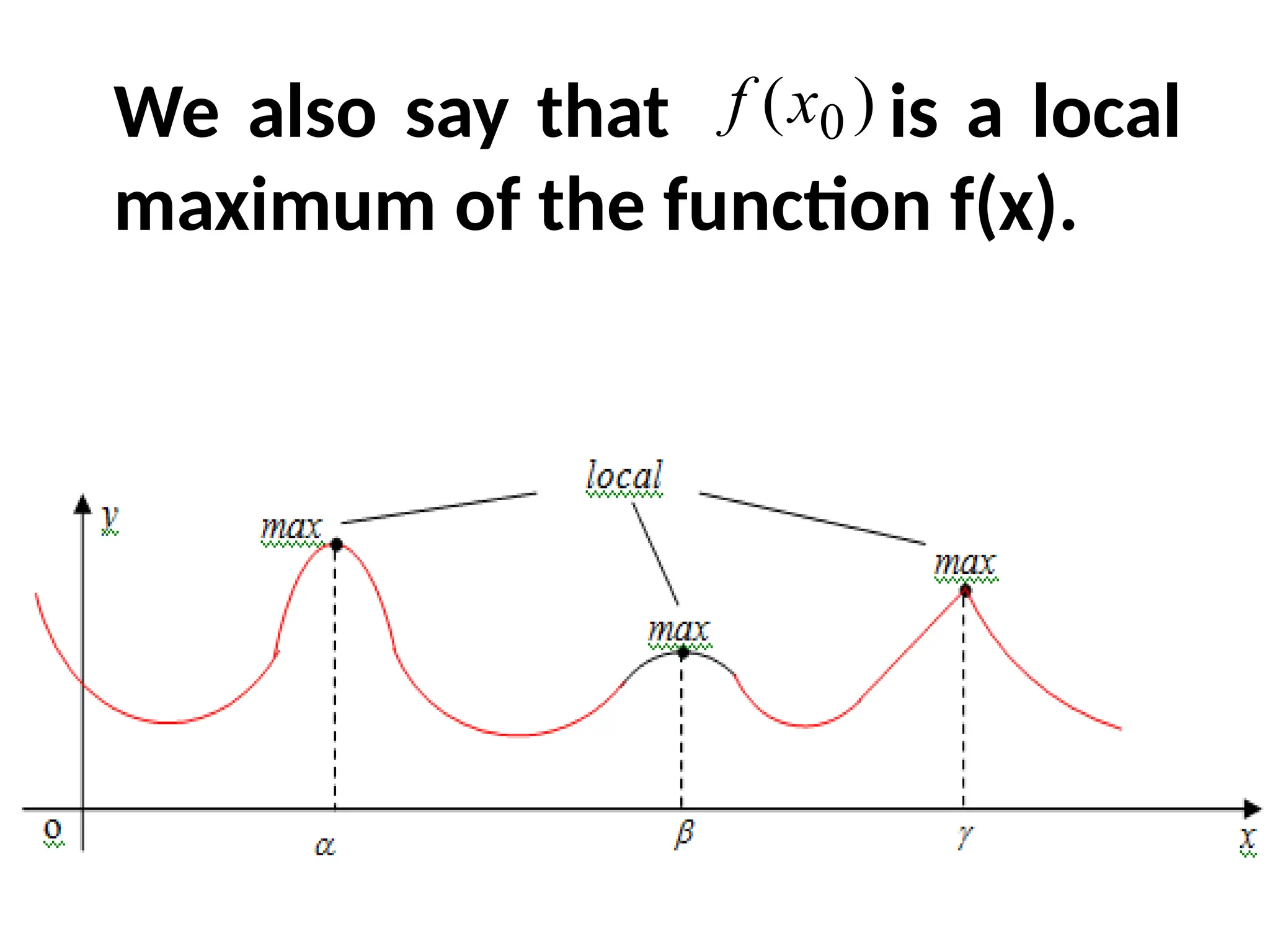
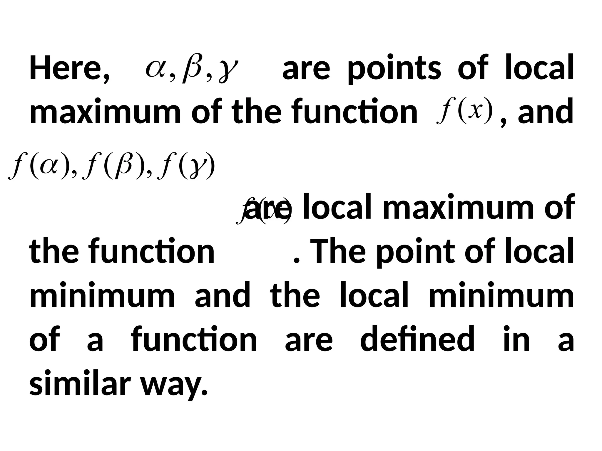
13. We also say that is a local
maximum of the function f(x).
)
( 0
x
f

14. Here, are points of local
maximum of the function , and
are local maximum of
the function . The point of local
minimum and the local minimum
of a function are defined in a
similar way.
)
(x
f


 ,
,
)
(x
f
)
(
),
(
),
( 

 f
f
f

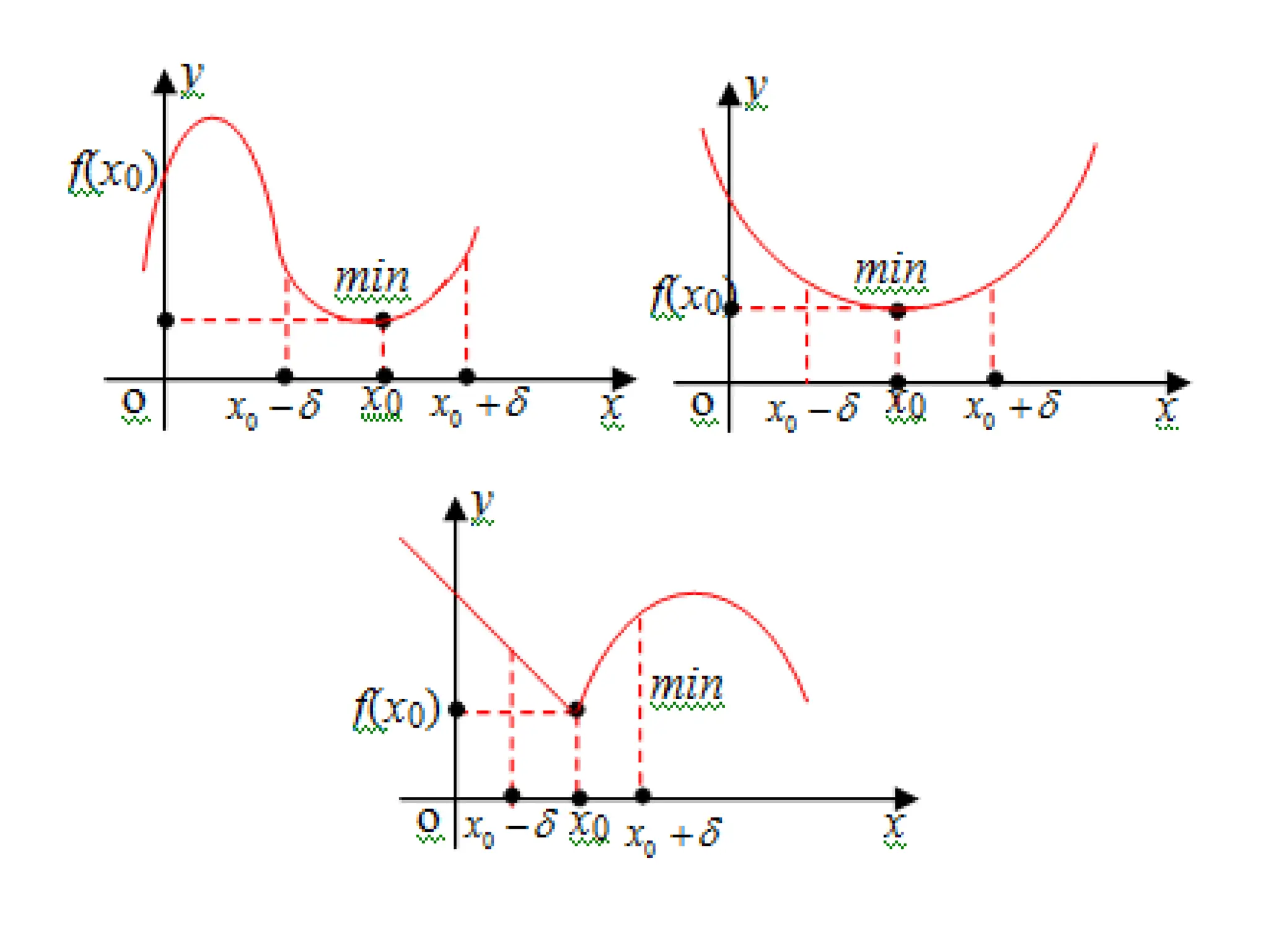
15. Definition: A point is called a point
of local minimum of the function ,
if the value is the least value of
the function in a neighbourhood
of the point .
In other words, it means that there
exist a - neighbourhood, , of
the point , such
that for all .
0
x
)
(x
f
)
( 0
x
f
)
(x
f
0
x
 0


0
x
)
,
(
)
( 0
0
0 

 

 x
x
x
U
)
(
)
(
)
( 0
0 x
f
x
f
x
U
x 
 

17. We also say that is a local
minimum of the function .
)
( 0
x
f
)
(x
f

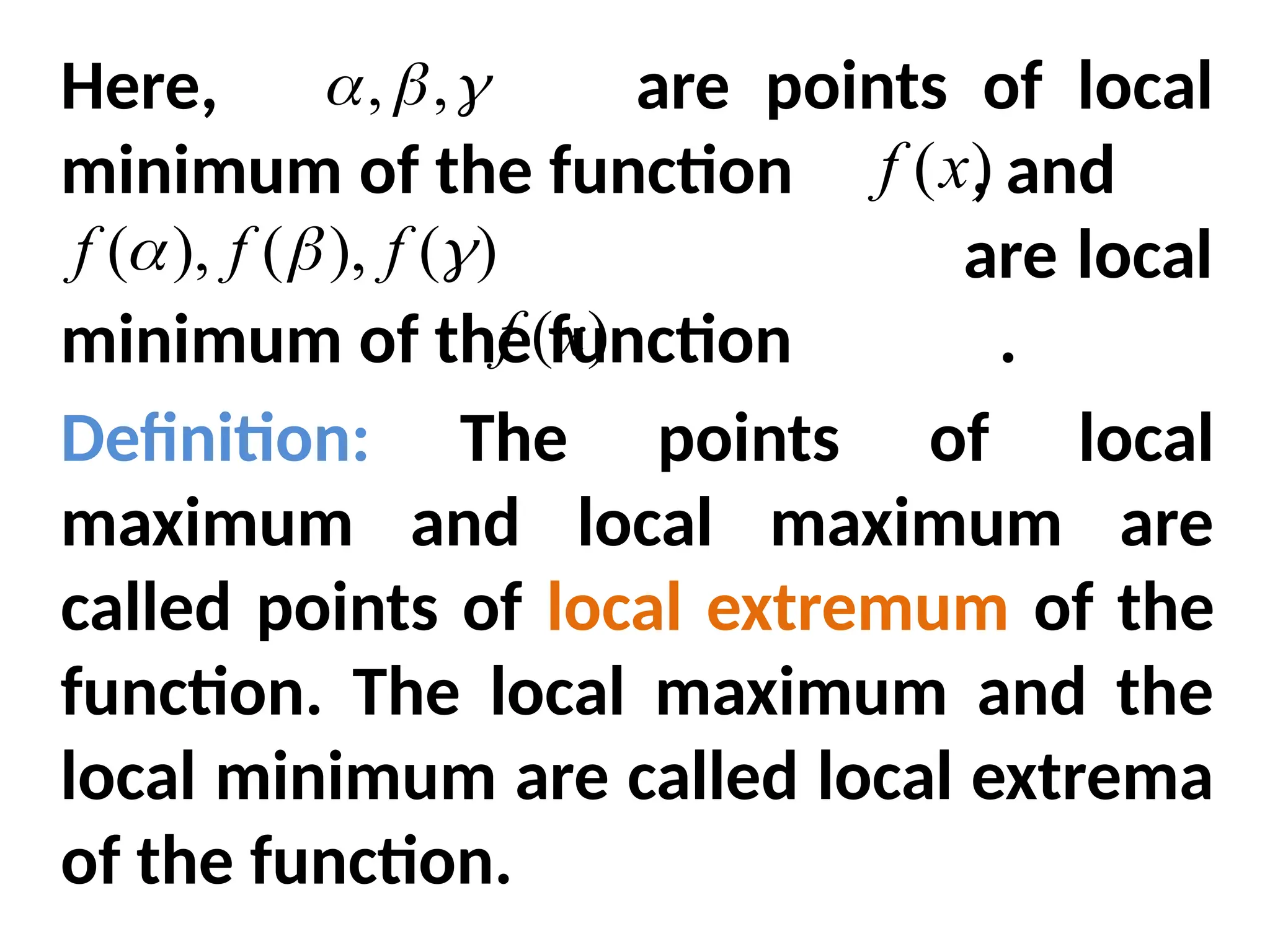
18. Here, are points of local
minimum of the function , and
are local
minimum of the function .
Definition: The points of local
maximum and local maximum are
called points of local extremum of the
function. The local maximum and the
local minimum are called local extrema
of the function.


 ,
,
)
(x
f
)
(x
f
)
(
),
(
),
( 

 f
f
f

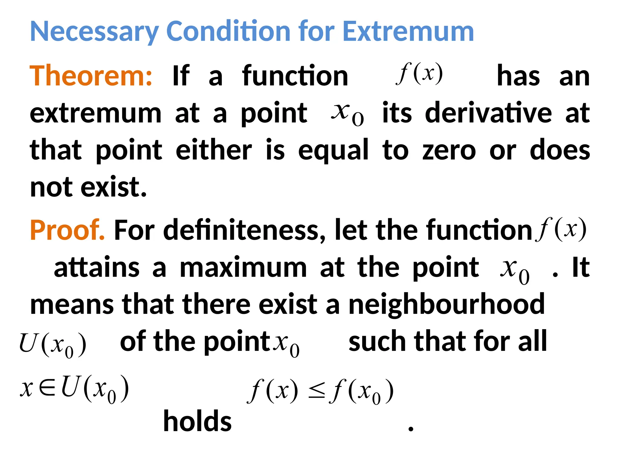
19. Necessary Condition for Extremum
Theorem: If a function has an
extremum at a point its derivative at
that point either is equal to zero or does
not exist.
Proof. For definiteness, let the function
attains a maximum at the point . It
means that there exist a neighbourhood
of the point such that for all
holds .
)
(x
f
)
(x
f
0
x
0
x
0
x
)
( 0
x
U
)
( 0
x
U
x )
(
)
( 0
x
f
x
f 

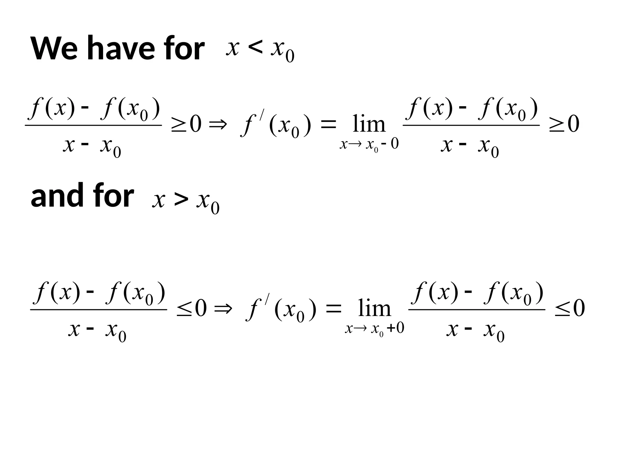
20. We have for
and for
0
)
(
)
(
lim
)
(
0
)
(
)
(
0
0
0
0
/
0
0
0









 x
x
x
f
x
f
x
f
x
x
x
f
x
f
x
x
0
x
x 
0
x
x 
0
)
(
)
(
lim
)
(
0
)
(
)
(
0
0
0
0
/
0
0
0









 x
x
x
f
x
f
x
f
x
x
x
f
x
f
x
x

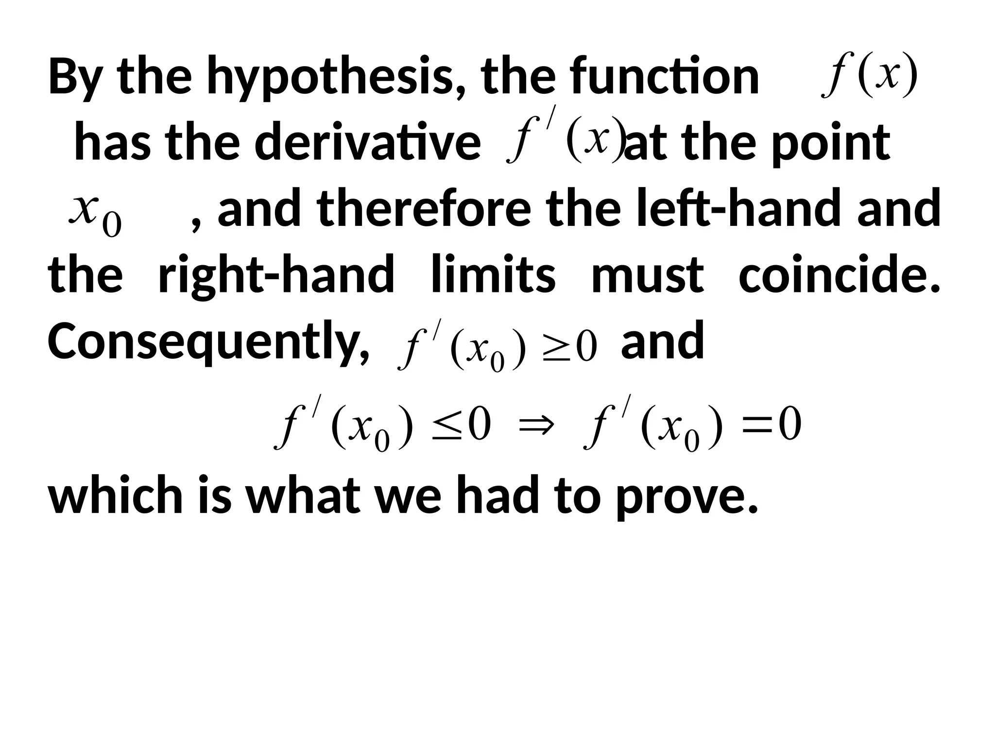
21. By the hypothesis, the function
has the derivative at the point
, and therefore the left-hand and
the right-hand limits must coincide.
Consequently, and
which is what we had to prove.
)
(x
f
)
(
/
x
f
0
x
0
)
( 0
/

x
f
0
)
(
0
)
( 0
/
0
/


 x
f
x
f

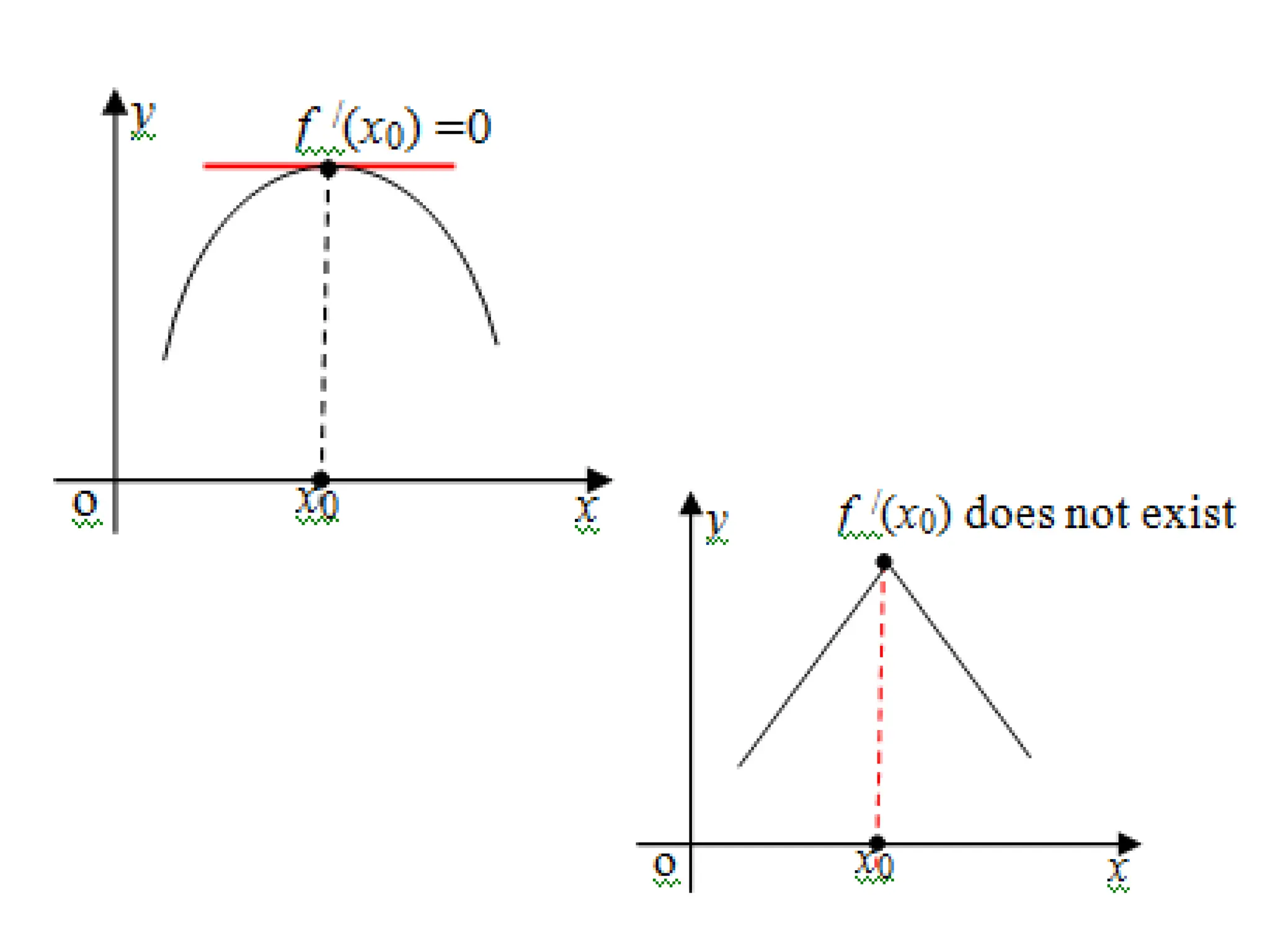
23. The argument is completely similar in
the case of a minimum.
Geometrically, the proved theorem
states that the tangent drawn to the
graph of a function at its highest or
lowest points is parallel to Ox (i.e.to
the axis of abscissas). It should be
noted that a function can also have
extrema at some of the points where
derivative does not exist.

24. Definition. A point at which the
derivative is equal to zero is called a
stationary point.
- stationary point
Definition. An interval point of the
domain of definition of the function at
which the derivative is equal to zero or
does not exist is called a critical point.
It is clear that every stationary point is
critical.
0
x
0
x
0
x
0
)
( 0
/

 x
f

25. The necessary condition for extremum
can be restated as follows.
Theorem: If is a point of extremum
then is a critical point. (i.e. every
point extremum is critical).
It should be noted that not every
critical point is a point of extremum.
0
x
0
x

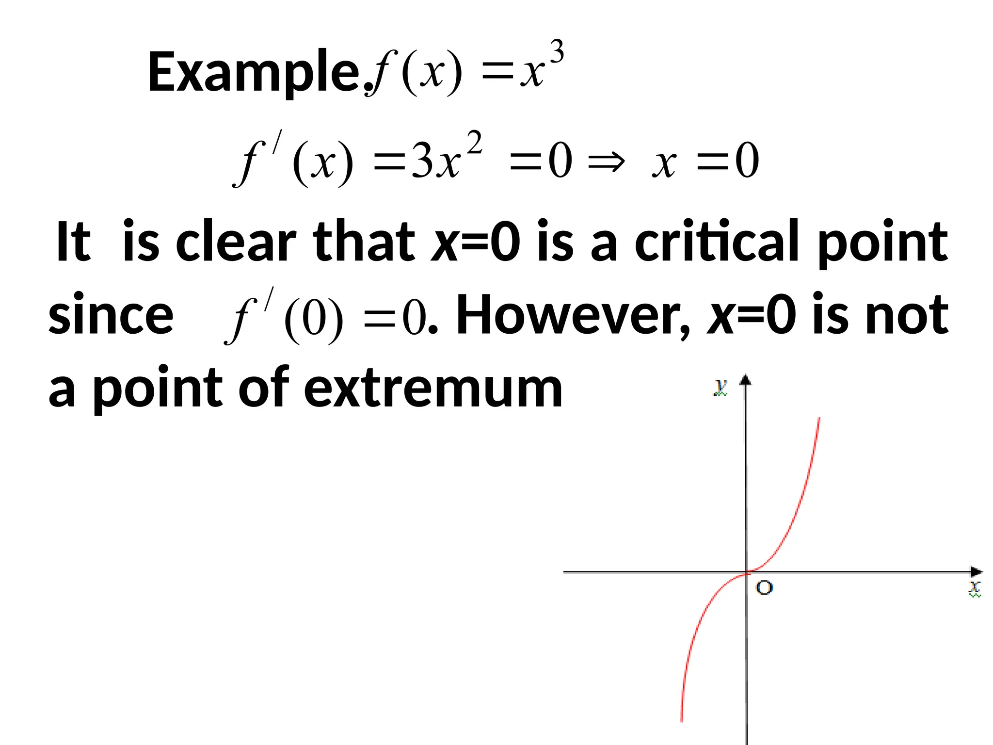
26. Example.
It is clear that x=0 is a critical point
since . However, x=0 is not
a point of extremum.
3
)
( x
x
f 
0
0
3
)
( 2
/



 x
x
x
f
0
)
0
(
/

f

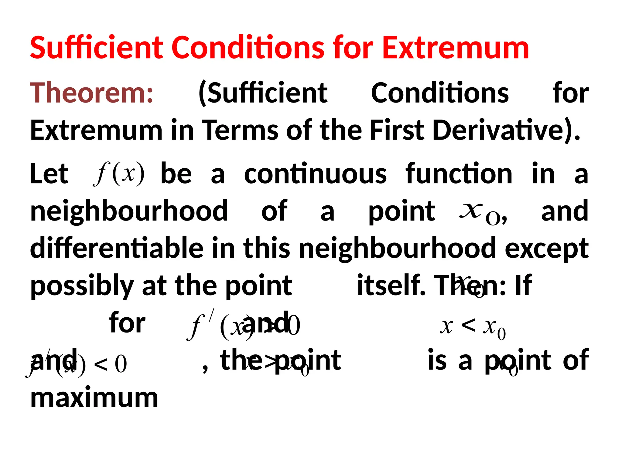
27. Sufficient Conditions for Extremum
Theorem: (Sufficient Conditions for
Extremum in Terms of the First Derivative).
Let be a continuous function in a
neighbourhood of a point , and
differentiable in this neighbourhood except
possibly at the point itself. Then: If
for and
and , the point is a point of
maximum
)
(x
f
0
x
0
x
0
x
0
)
(
/

x
f 0
x
x 
0
)
(
/

x
f 0
x
x 

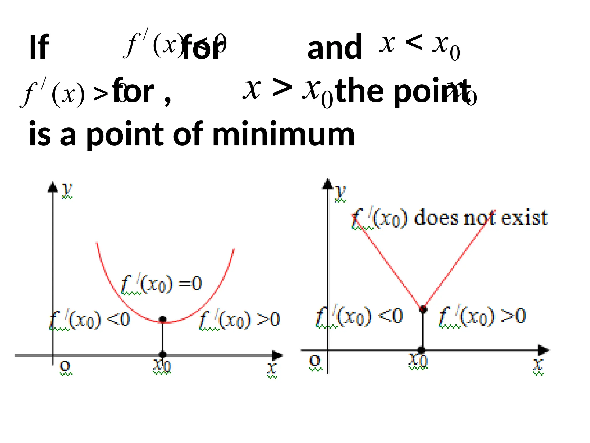
29. If for and
for , the point
is a point of minimum
0
)
(
/

x
f
0
x
x 
0
x
x 
0
)
(
/

x
f 0
x

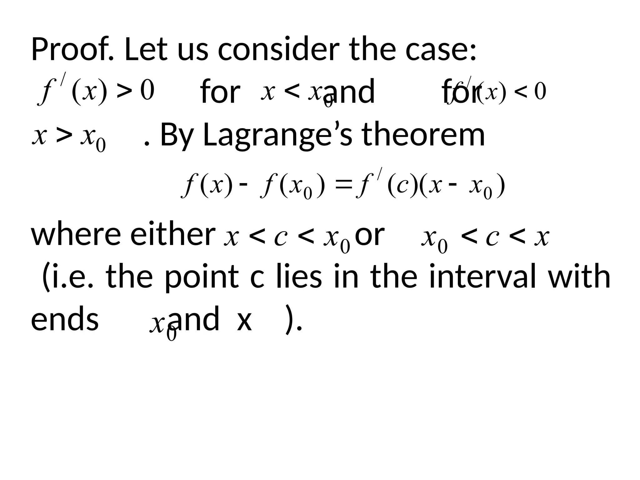
30. Proof. Let us consider the case:
for and for
. By Lagrange’s theorem
where either or
(i.e. the point c lies in the interval with
ends and x ).
0
)
(
/

x
f 0
x
x  0
)
(
/

x
f
0
x
x 
)
)(
(
)
(
)
( 0
/
0 x
x
c
f
x
f
x
f 


0
x
c
x 
 x
c
x 

0
0
x

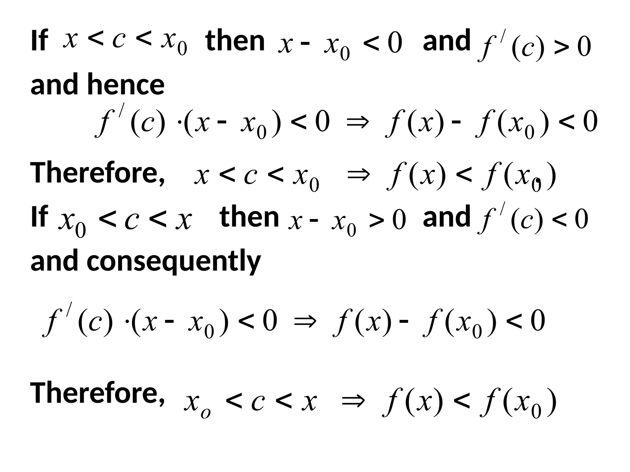
31. If then and
and hence
Therefore, .
If then and
and consequently
Therefore,
x
c
x 

0
0
x
c
x 
 0
0 
 x
x 0
)
(
/

c
f
0
)
(
)
(
0
)
(
)
( 0
0
/





 x
f
x
f
x
x
c
f
)
(
)
( 0
0 x
f
x
f
x
c
x 



0
0 
 x
x 0
)
(
/

c
f
0
)
(
)
(
0
)
(
)
( 0
0
/





 x
f
x
f
x
x
c
f
)
(
)
( 0
x
f
x
f
x
c
xo 




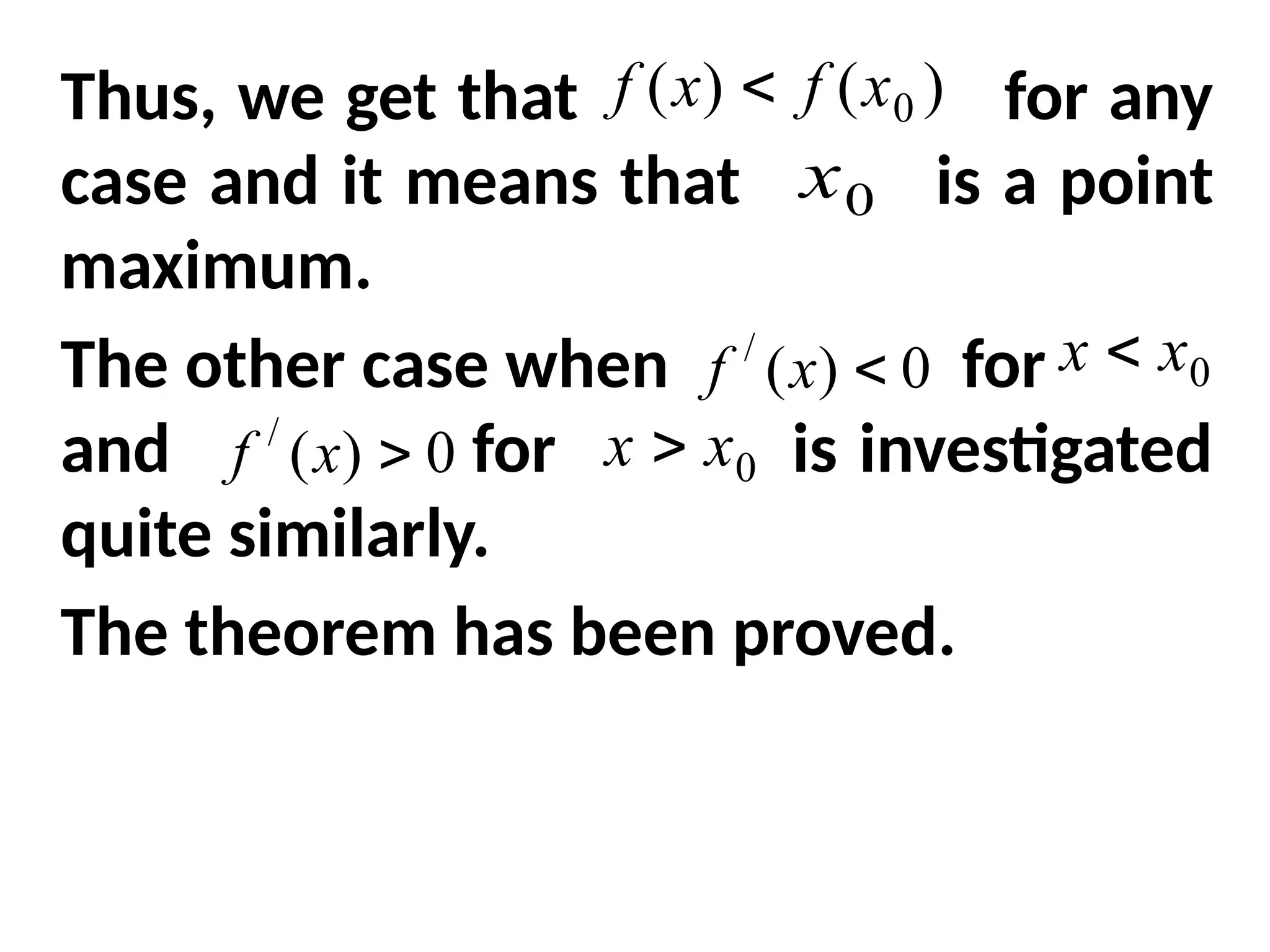
32. Thus, we get that for any
case and it means that is a point
maximum.
The other case when for
and for is investigated
quite similarly.
The theorem has been proved.
)
(
)
( 0
x
f
x
f 
0
x
0
)
(
/

x
f 0
x
x 
0
)
(
/

x
f 0
x
x 

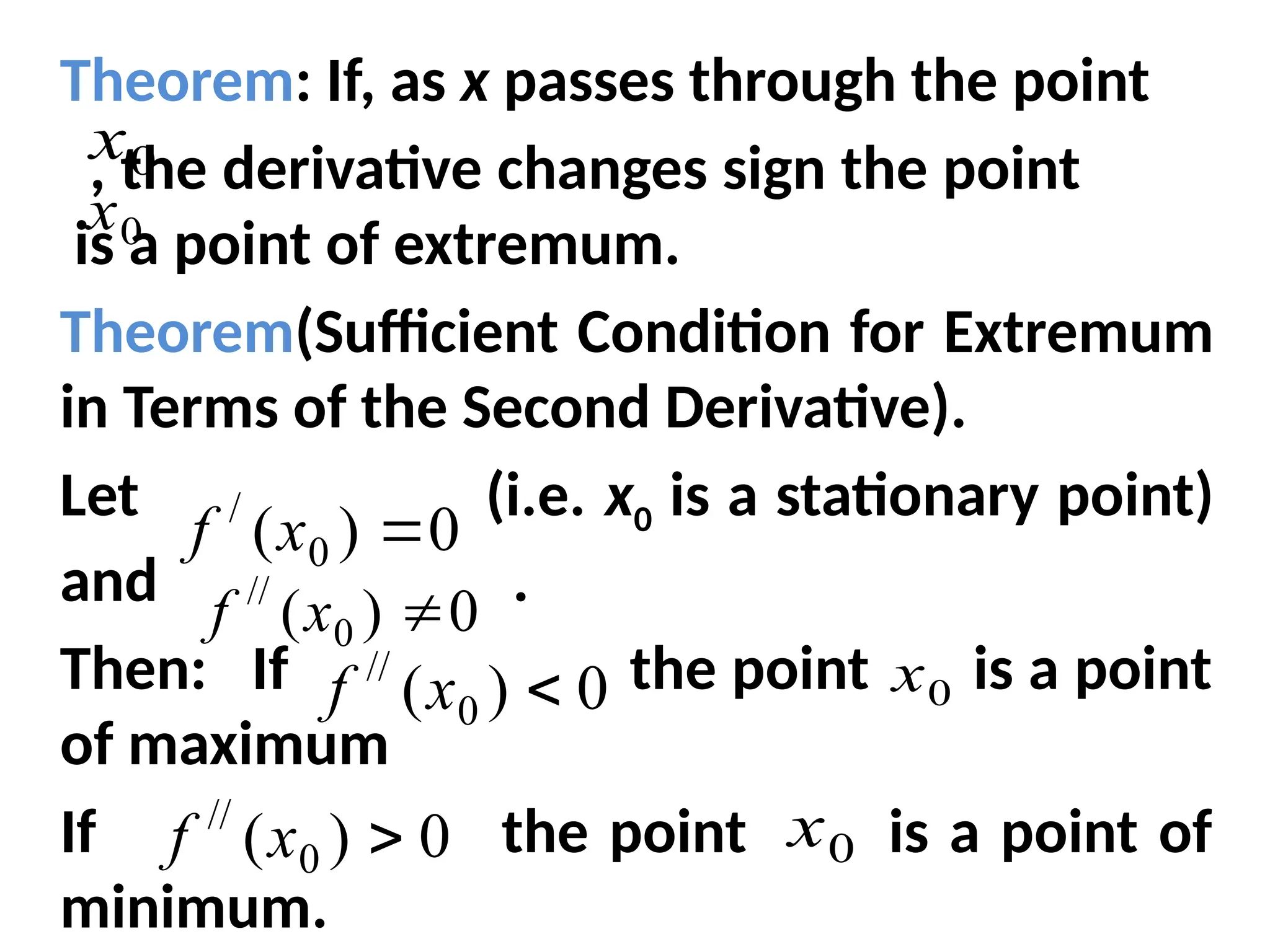
33. Theorem: If, as x passes through the point
, the derivative changes sign the point
is a point of extremum.
Theorem(Sufficient Condition for Extremum
in Terms of the Second Derivative).
Let (i.e. x0 is a stationary point)
and .
Then: If the point is a point
of maximum
If the point is a point of
minimum.
0
x
0
x
0
x
0
x
0
)
( 0
/

x
f
0
)
( 0
//

x
f
0
)
( 0
//

x
f
0
)
( 0
//

x
f

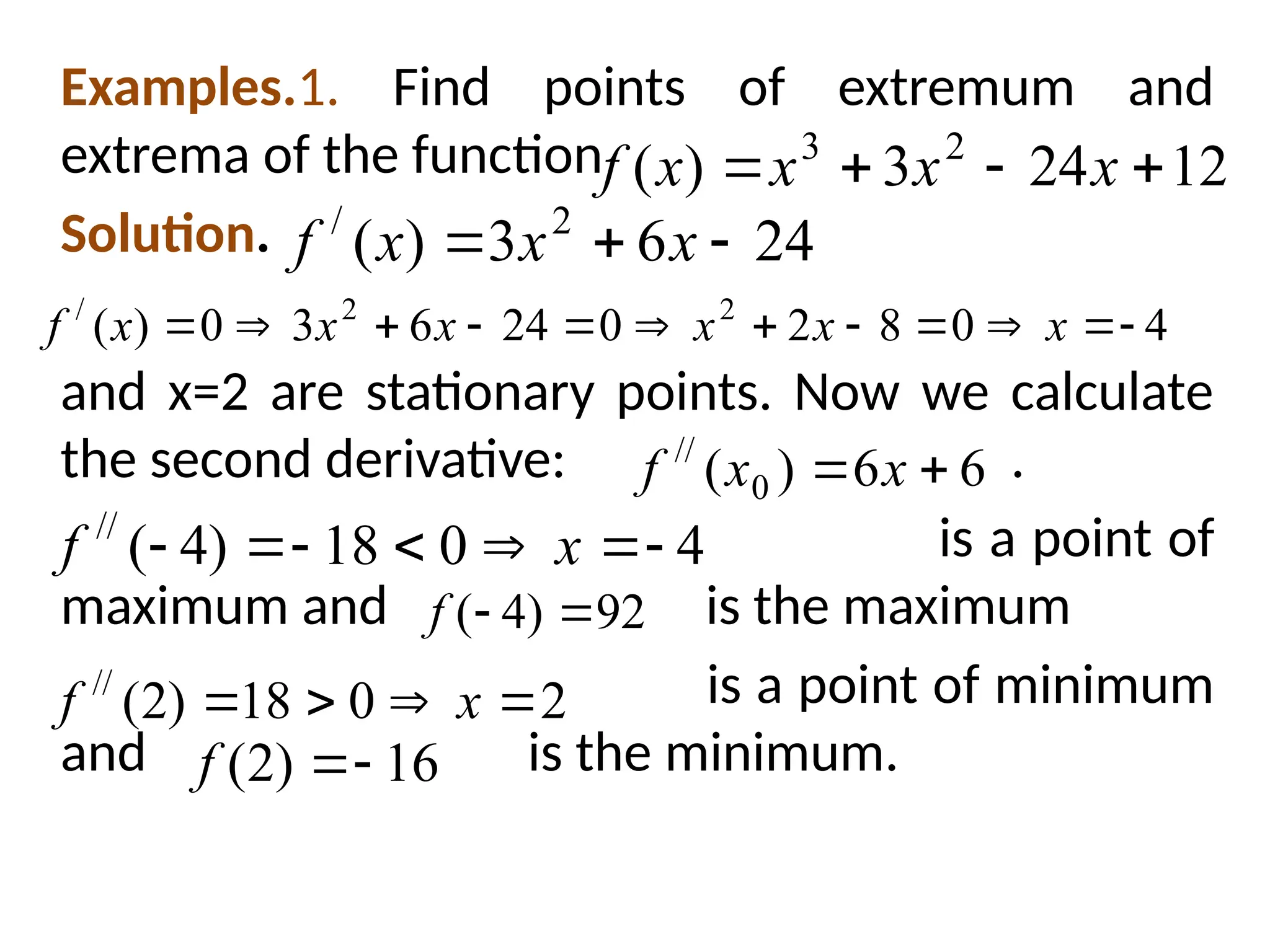
34. Examples.1. Find points of extremum and
extrema of the function
Solution.
and x=2 are stationary points. Now we calculate
the second derivative: .
is a point of
maximum and is the maximum
is a point of minimum
and is the minimum.
12
24
3
)
( 2
3



 x
x
x
x
f
24
6
3
)
( 2
/


 x
x
x
f
4
0
8
2
0
24
6
3
0
)
( 2
2
/











 x
x
x
x
x
x
f
6
6
)
( 0
//

 x
x
f
4
0
18
)
4
(
//






 x
f
92
)
4
( 

f
2
0
18
)
2
(
//



 x
f
16
)
2
( 

f

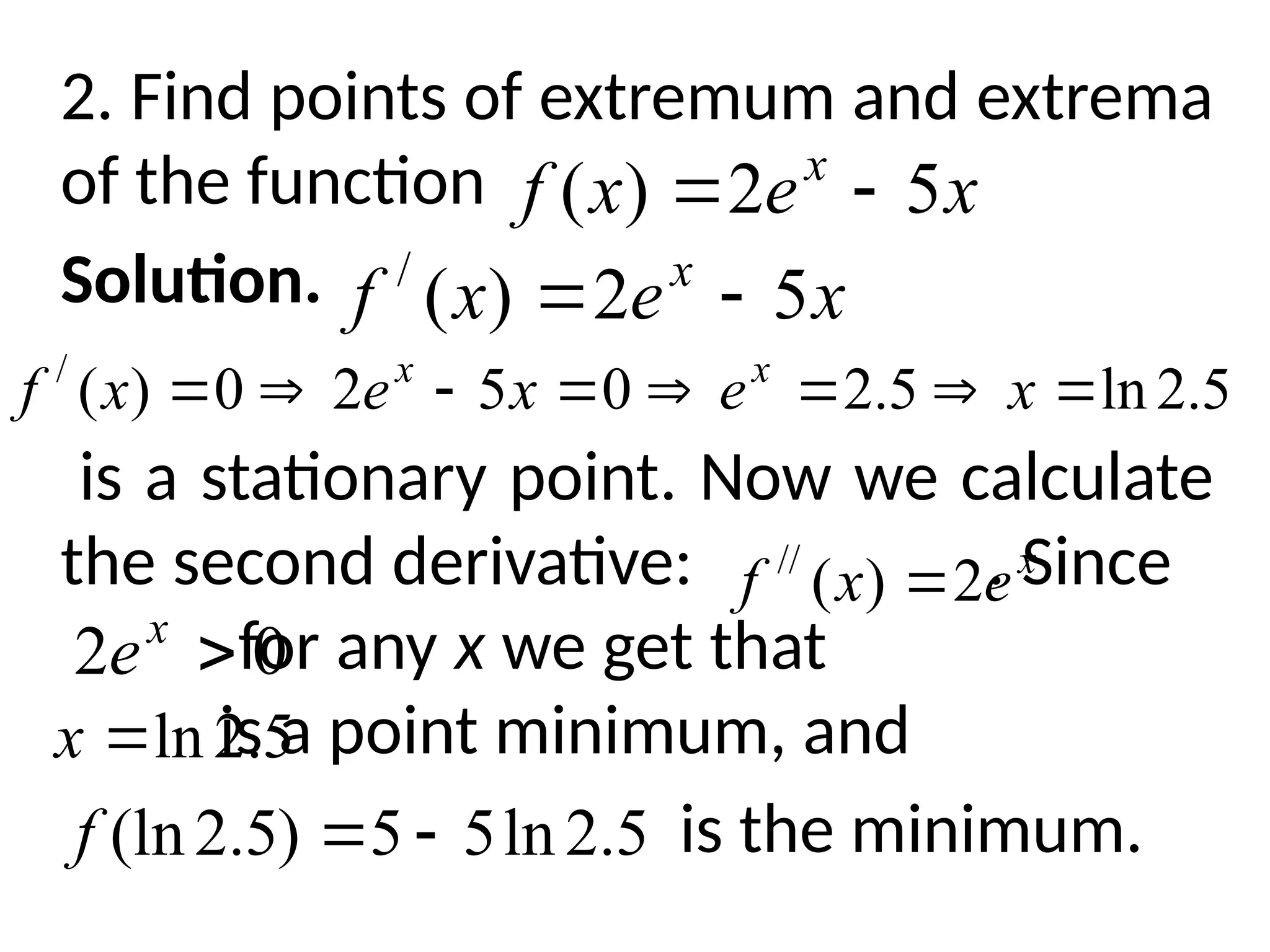
35. 2. Find points of extremum and extrema
of the function
Solution.
is a stationary point. Now we calculate
the second derivative: . Since
for any x we get that
is a point minimum, and
is the minimum.
x
e
x
f x
5
2
)
( 

x
e
x
f x
5
2
)
(
/


5
.
2
ln
5
.
2
0
5
2
0
)
(
/







 x
e
x
e
x
f x
x
x
e
x
f 2
)
(
//

0
2 
x
e
5
.
2
ln

x
5
.
2
ln
5
5
)
5
.
2
(ln 

f

36. The Greatest and the Least Values of a Function
Suppose it is necessary to find the
greatest and the least values of the
function on a closed interval
.
According to well-known Weierstrass’s
theorem:
)
(x
f
y 
]
,
[ b
a

37. Theorem: A continuous function
defined over a closed interval is
bounded and attains its least value and
its greatest value. In other words, it
means that there exist at least one
point and at least one point
such that at these points the
function attains, respectively, its
greatest and least values
and
]
,
[
1 b
a
c 
]
,
[
2 b
a
c 
M
x
f
c
f
b
x
a




)
(
max
)
( 1 m
x
f
c
f
b
x
a




)
(
min
)
( 2

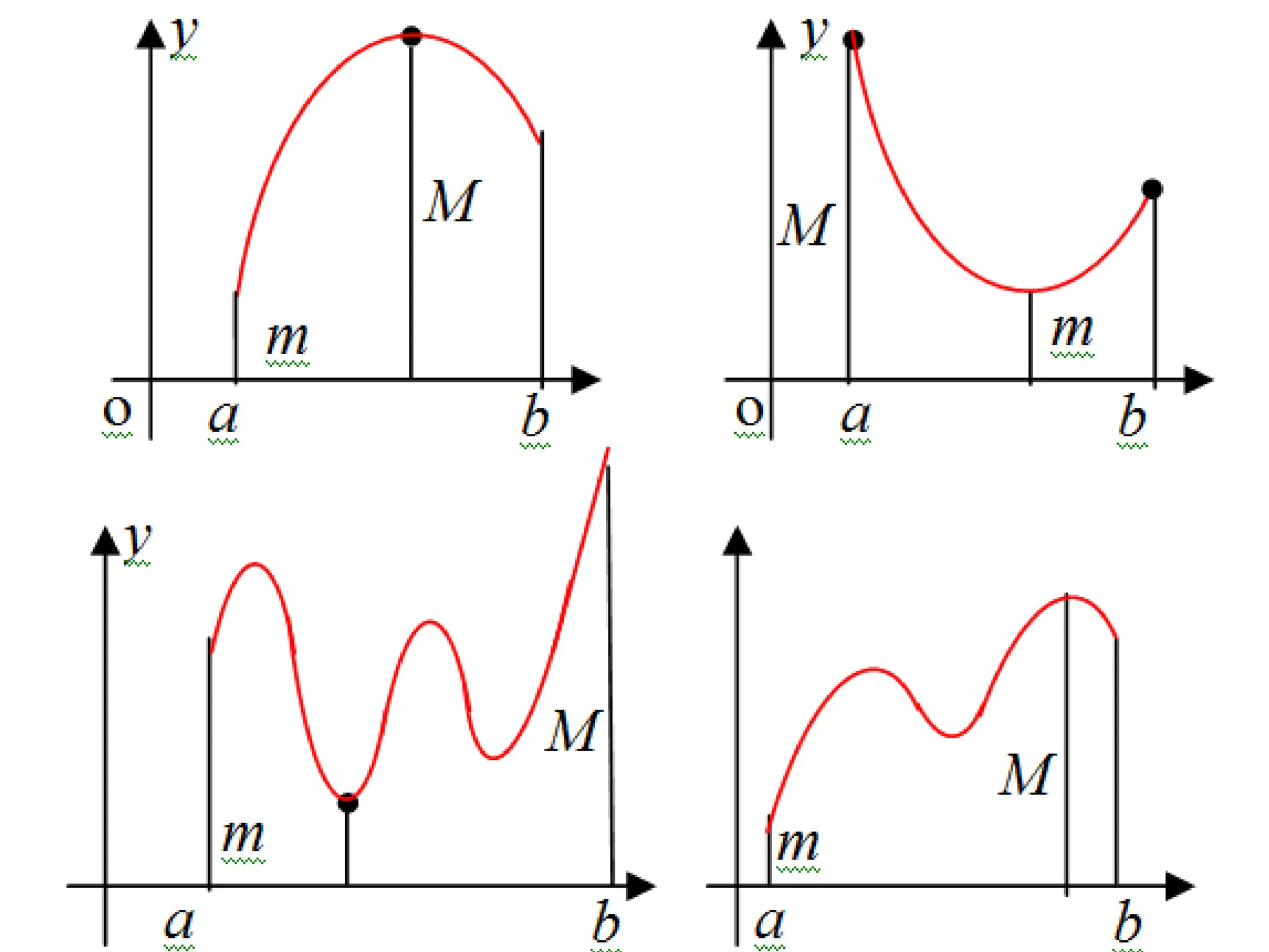
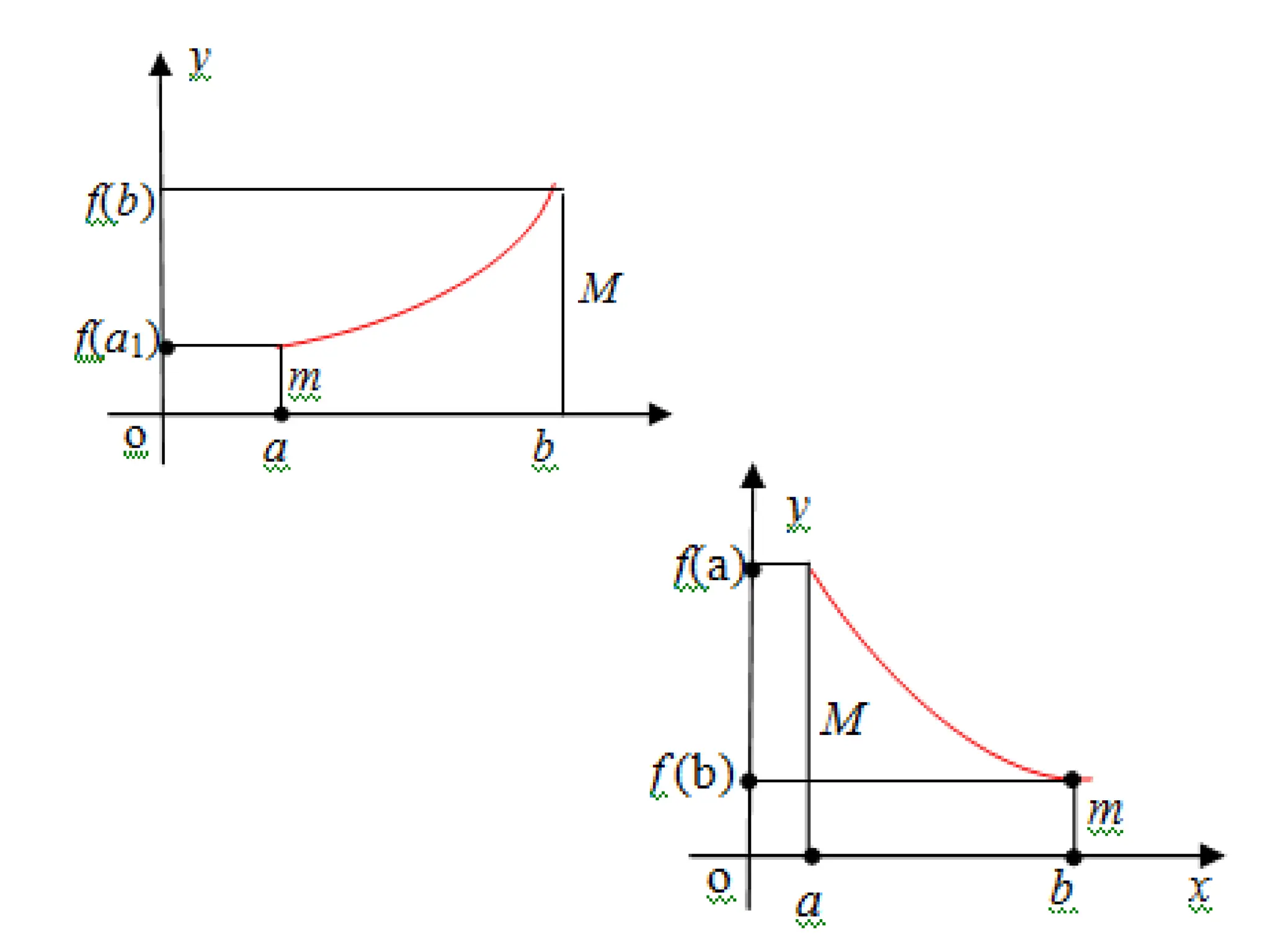
38. We are interested in the question of “How
to find these points?”. Suppose, at first, a
function has no critical points. In that case
the function is monotone.
It is clear that when a function y=f(x)
is monotone in a closed interval [a,b] its
greatest value is M=f(b) and the least value
is m=f(a) if the function increases and,
conversely, the greatest value is M=f(a) and
the least value is m=f(b) if the function
decreases.

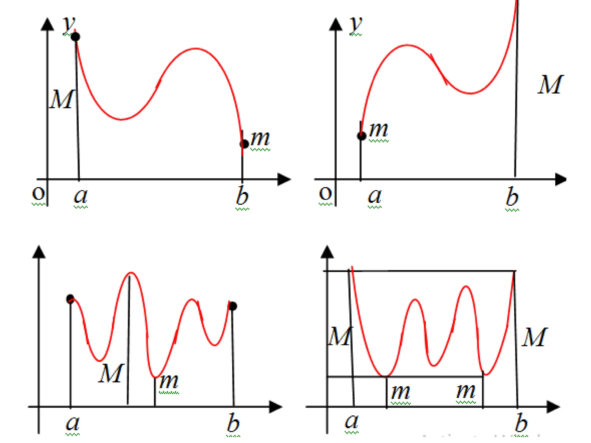
40. Now suppose a function has a finite
number of critical points in [a,b]. These
points divide the closed interval [a,b]
into finite number of segments, in
which there are no critical points.
Therefore, the greatest and the least
values of the function on these
segments are assumed at their ends,
i.e. at critical points or at points a and
b.

43. We are now ready to formulate the rule
(algorithm). For the case when a function
is not only continuous on a closed interval
[a,b], but it has a finite number of critical
points in [a,b], we specify the rule for
finding the greatest and the least values.
In order to find the greatest and the least
values of a function, y=f(x) on a closed
interval [a,b] and having a finite number
of critical points in [a,b], you need to:

44. 1.Find the critical points belonging
to [a,b].
2. Calculate the values of the
function at these critical points and
the values of the function at the end
points, i.e. f(a) and f(b) .
3. Choose from the values obtained
the greatest and the least values.

45. Example.
Find the greatest and the least values of the
function on the interval [0,2]
Solution. To find the critical points, first find
the derivative . Solving the
equation we get . It
follows that in the closed interval [0,2] there
is only one critical point x=1. Recall that a
critical point must be internal and cannot be
one of the end point of the segment.
3
5
5
3
)
( x
x
x
f 

2
4
/
15
15
)
( x
x
x
f 

0
)
(
/

x
f 1
,
0 

 x
x

46. Now we calculate and
. Comparing these values we get
and
2. Find the greatest and the least values of
the function on the
interval [-2,3].
Solution. We find the derivative
2
)
1
(
,
0
)
0
( 

 f
f
56
)
2
( 
f
56
)
2
(
)
(
max
]
2
,
0
[

 f
x
f 2
)
1
(
)
(
min
]
2
,
0
[


 f
x
f
3
3
)
( x
x
x
f 

2
/
3
3
)
( x
x
f 

1
0
3
3
0
)
( 2
/






 x
x
x
f

47. Points are critical points.
Now we calculate the values of the function
at these points: . We
also calculate the values of the function at
the and points: . From
the resulting four values we choose the
greatest and the least. Thus, we have
and
1


x
2
)
1
(
,
2
)
1
( 


 f
f
18
)
3
(
,
2
)
2
( 


 f
f
2
)
1
(
)
2
(
)
(
max
]
3
,
2
[





f
f
x
f
18
)
3
(
)
(
min
]
3
,
2
[




f
x
f