The document discusses the Laplacian of Gaussian (LoG) filter and how it can be used for edge detection and blob detection in images. The LoG filter applies a Gaussian blur to smooth the image, then takes the Laplacian to find zero-crossings, which indicate edges. It can also detect blobs by finding local extrema (maxima and minima) in the LoG filtered image. The scale of blobs detected depends on the sigma value used for the Gaussian blur. So the LoG filter acts as a band-pass filter, suppressing high and low frequencies to detect objects of a particular scale in the image.

1. Robert Collins
CSE486
Lecture 11:
LoG and DoG Filters

2. Robert Collins
CSE486
Today’s Topics
Laplacian of Gaussian (LoG) Filter
- useful for finding edges
- also useful for finding blobs!
approximation using Difference of Gaussian (DoG)

3. Robert Collins
Recall: First Derivative Filters
CSE486
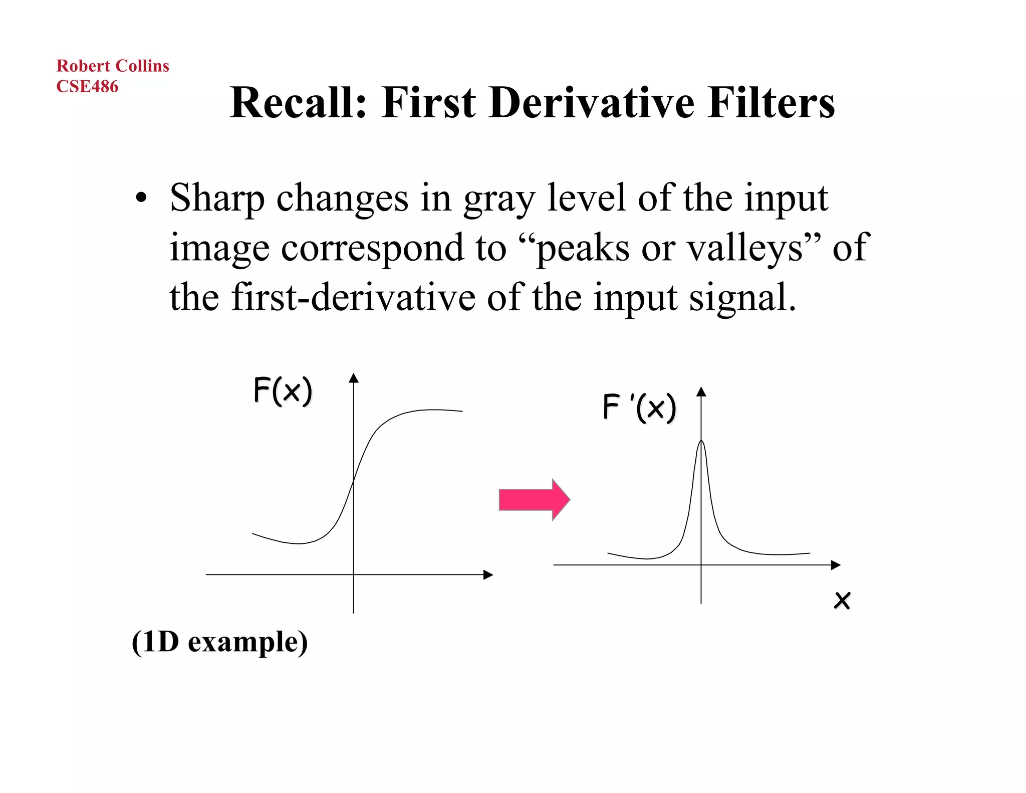
• Sharp changes in gray level of the input
image correspond to “peaks or valleys” of
the first-derivative of the input signal.
F(x)
F ’(x)
x
(1D example)
O.Camps, PSU

4. Robert Collins
CSE486
Second-Derivative Filters
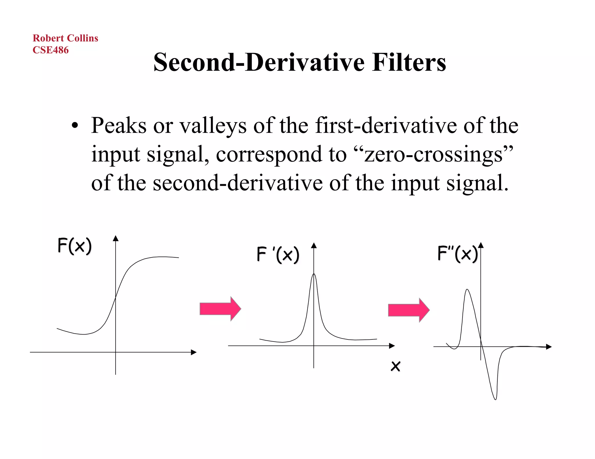
• Peaks or valleys of the first-derivative of the
input signal, correspond to “zero-crossings”
of the second-derivative of the input signal.
F(x) F ’(x) F’’(x)
x
O.Camps, PSU

5. Robert Collins
CSE486
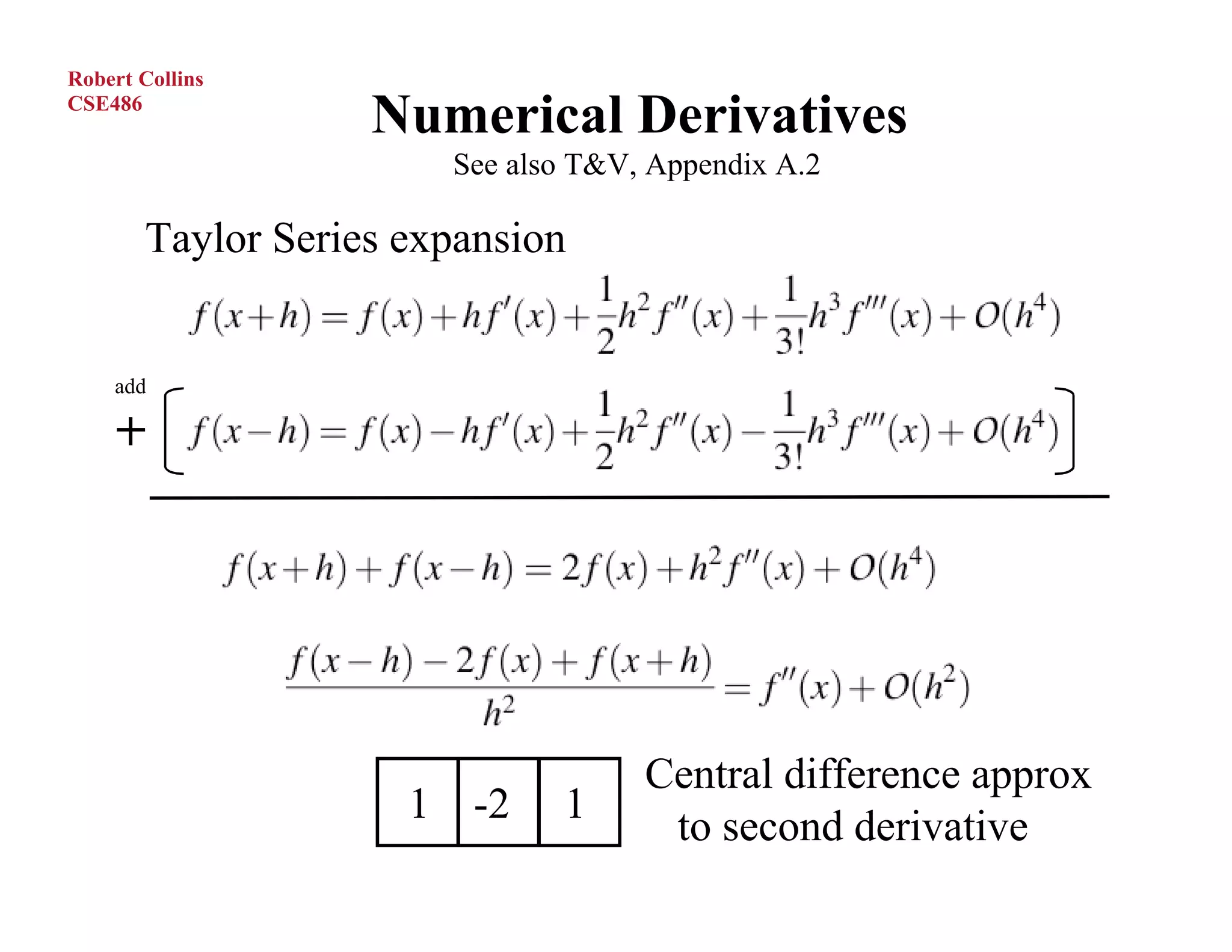
Numerical Derivatives
See also T&V, Appendix A.2
Taylor Series expansion
add
Central difference approx
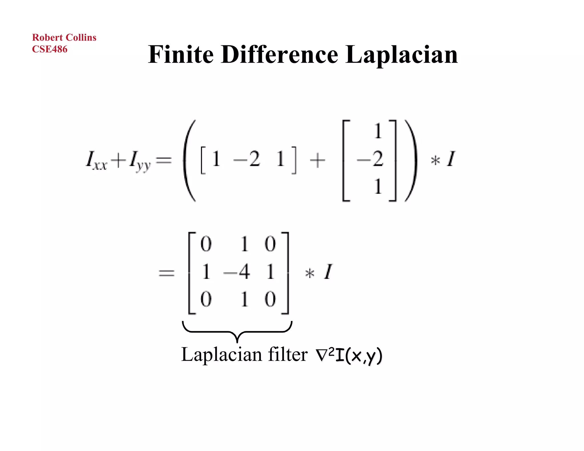
1 -2 1
to second derivative

6. Robert Collins
CSE486
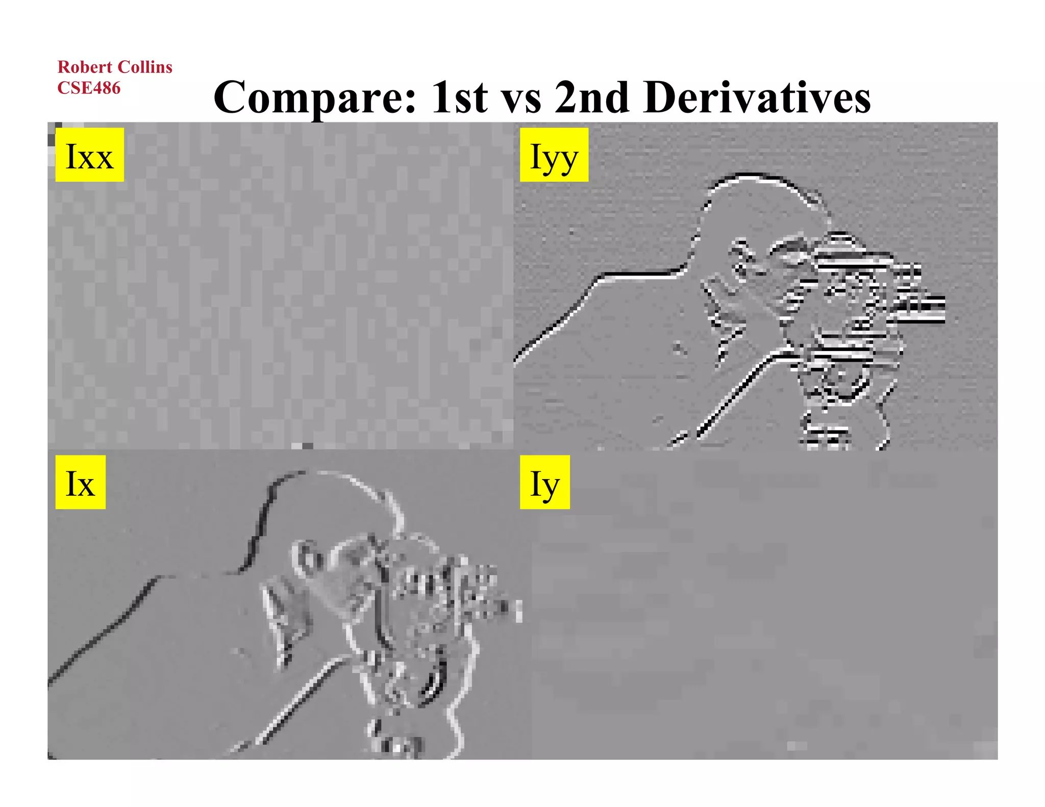
Example: Second Derivatives
Ixx=d2I(x,y)/dx2
[ 1 -2 1 ]
I(x,y)
2nd Partial deriv wrt x
1
-2
1 Iyy=d2I(x,y)/dy2
2nd Partial deriv wrt y

7. Robert Collins
CSE486
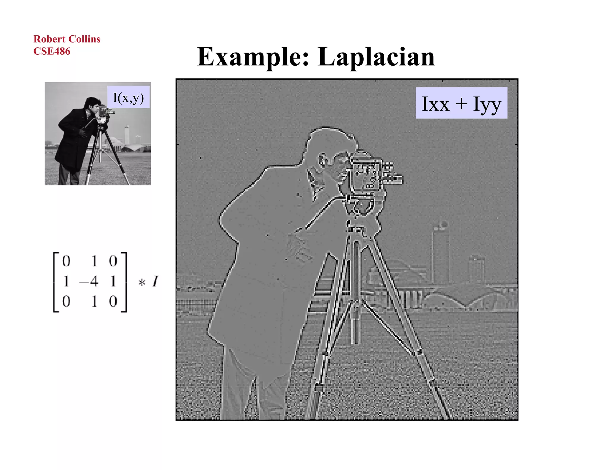
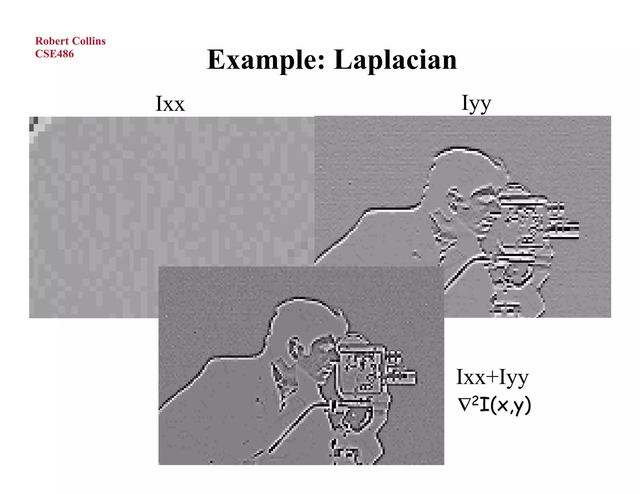
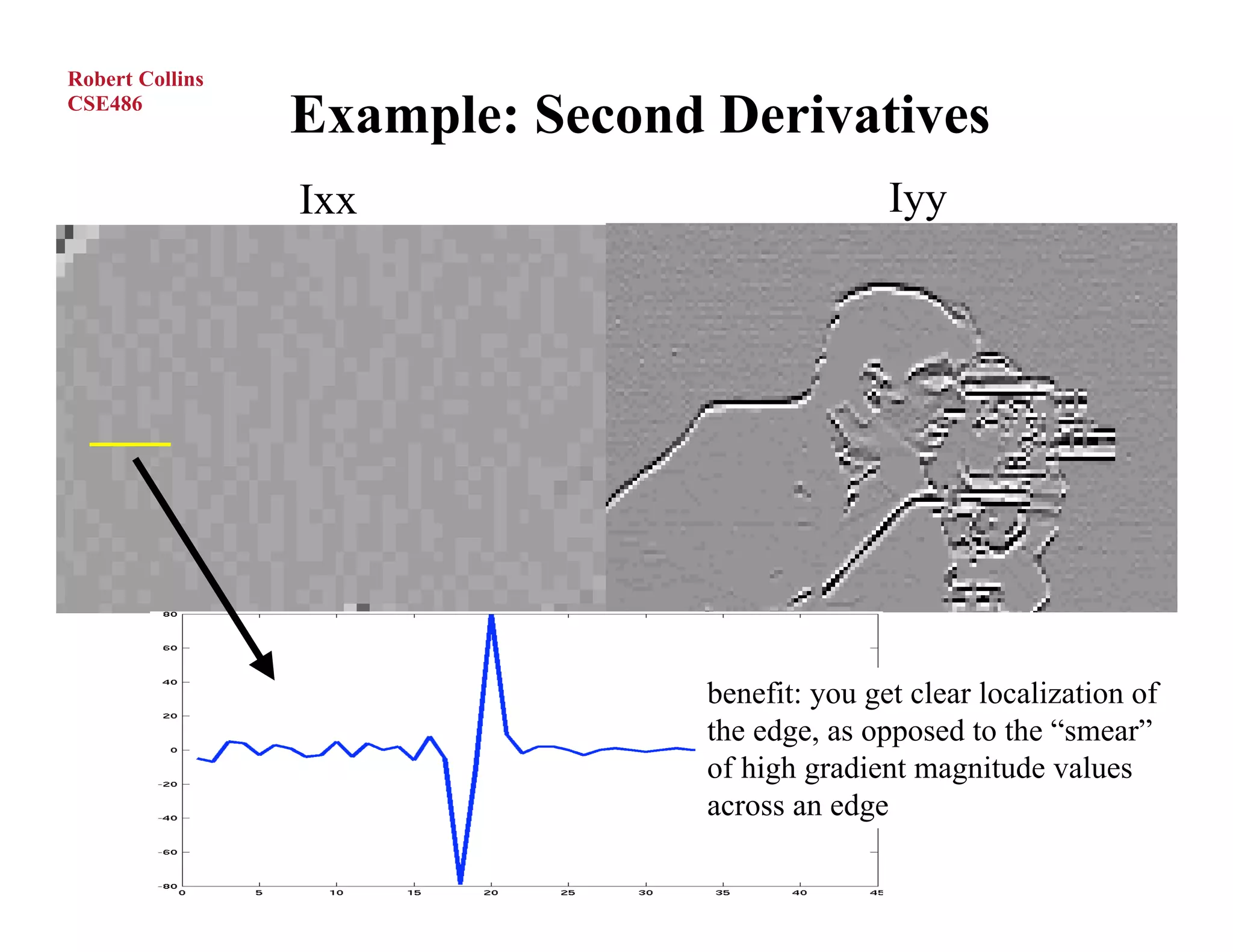
Example: Second Derivatives
Ixx Iyy
benefit: you get clear localization of
the edge, as opposed to the “smear”
of high gradient magnitude values
across an edge

8. Robert Collins
CSE486
Compare: 1st vs 2nd Derivatives
Ixx Iyy
Ix Iy

9. Robert Collins
CSE486
Finding Zero-Crossings
An alternative approx to finding edges as peaks in
first deriv is to find zero-crossings in second deriv.
In 1D, convolve with [1 -2 1] and look for pixels
where response is (nearly) zero?
Problem: when first deriv is zero, so is second. I.e.
the filter [1 -2 1] also produces zero when convolved
with regions of constant intensity.
So, in 1D, convolve with [1 -2 1] and look for pixels
where response is nearly zero AND magnitude of
first derivative is “large enough”.

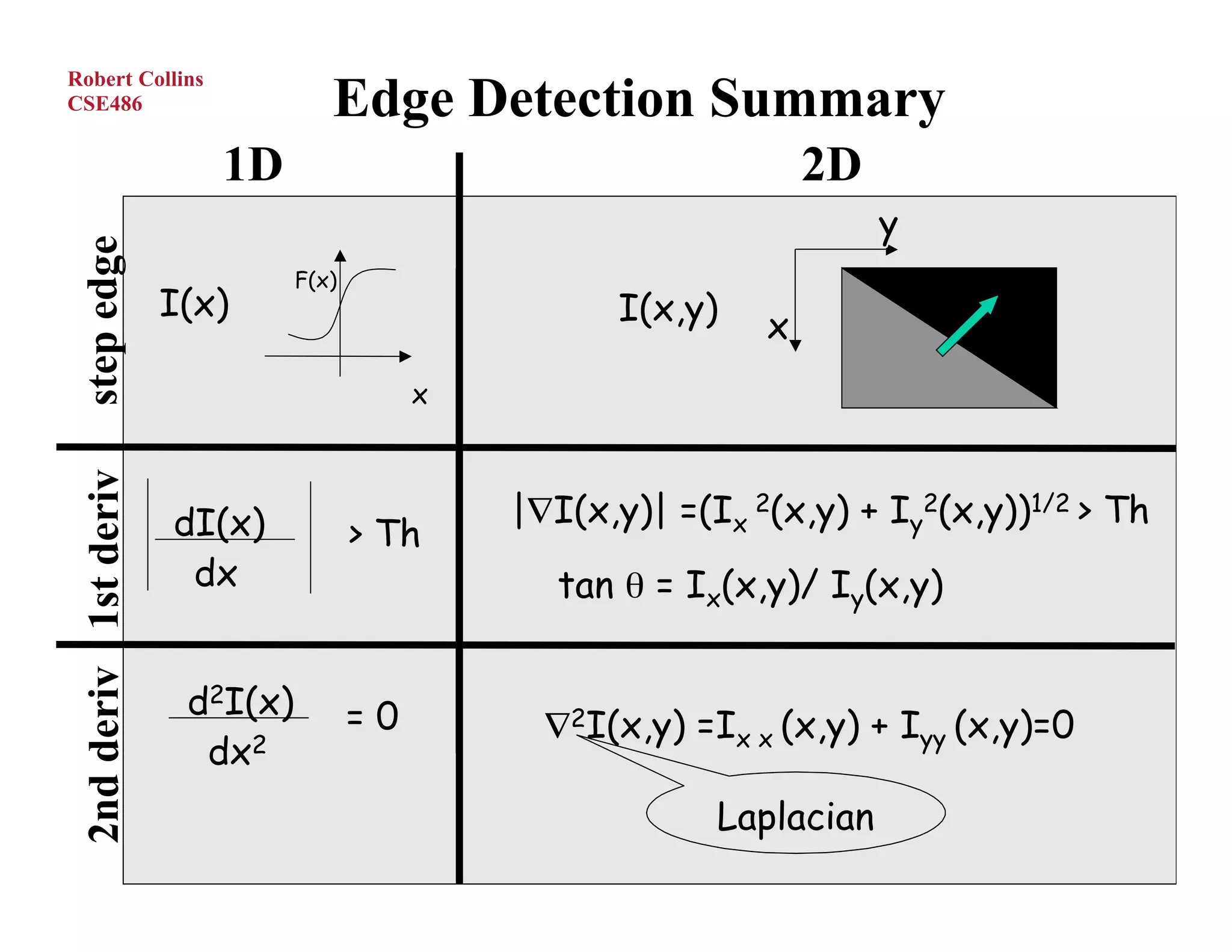
10. Edge Detection Summary
Robert Collins
CSE486
1D 2D
y
step edge
F(x)
I(x) I(x,y) x
x
2nd deriv 1st deriv
dI(x) |∇I(x,y)| =(Ix 2(x,y) + Iy2(x,y))1/2 > Th
> Th
dx tan θ = Ix(x,y)/ Iy(x,y)
d2I(x) =0 ∇2I(x,y) =Ix x (x,y) + Iyy (x,y)=0
dx2
Laplacian

11. Robert Collins
CSE486
Finite Difference Laplacian
Laplacian filter ∇2I(x,y)

12. Robert Collins
CSE486
Example: Laplacian
I(x,y)
Ixx + Iyy

13. Robert Collins
CSE486
Example: Laplacian
Ixx Iyy
Ixx+Iyy
∇2I(x,y)

14. Robert Collins
CSE486
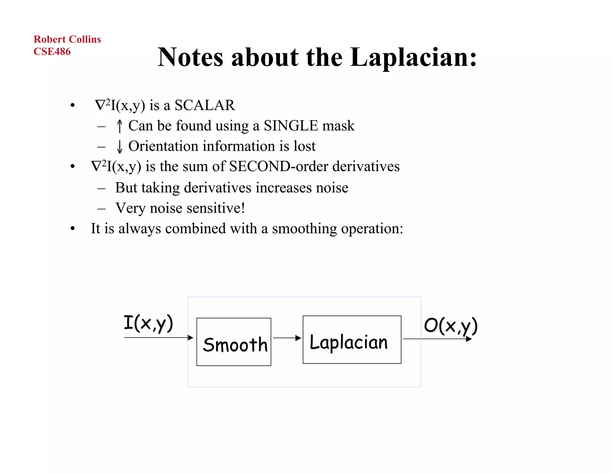
Notes about the Laplacian:
• ∇2I(x,y) is a SCALAR
– ↑ Can be found using a SINGLE mask
– ↓ Orientation information is lost
• ∇2I(x,y) is the sum of SECOND-order derivatives
– But taking derivatives increases noise
– Very noise sensitive!
• It is always combined with a smoothing operation:
I(x,y) O(x,y)
Smooth Laplacian
O.Camps, PSU

15. Robert Collins
CSE486
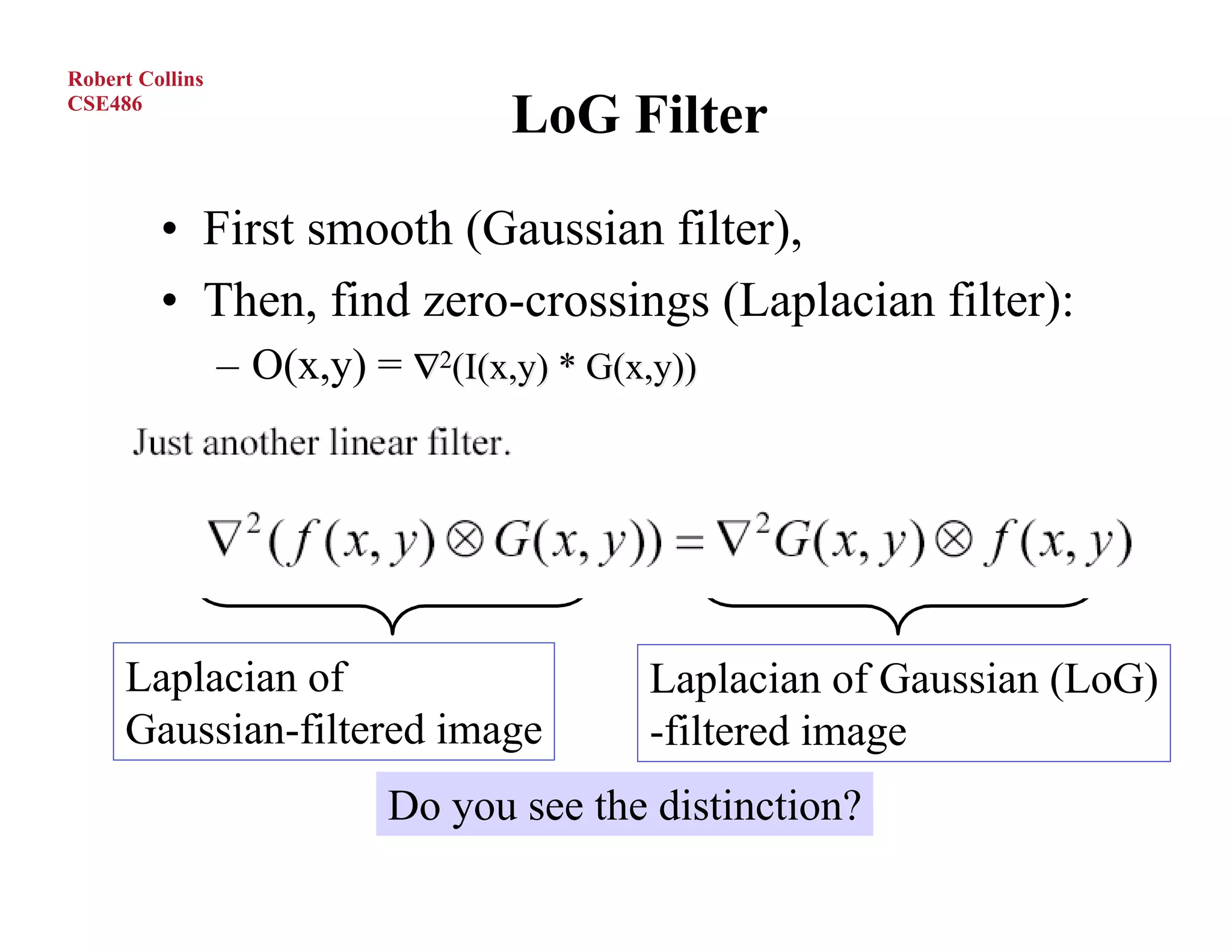
LoG Filter
• First smooth (Gaussian filter),
• Then, find zero-crossings (Laplacian filter):
– O(x,y) = ∇2(I(x,y) * G(x,y))
Laplacian of Laplacian of Gaussian (LoG)
Gaussian-filtered image -filtered image
Do you see the distinction?
O.Camps, PSU

16. Robert Collins
CSE486
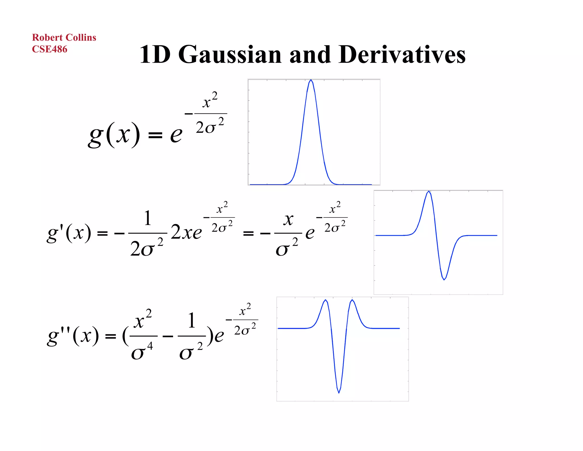
1D Gaussian and Derivatives
x2
−
2σ 2
g ( x) = e
x2 x2
1 − 2 x − 2
g ' ( x) = − 2 2 xe 2σ
=− 2 e 2σ
2σ σ
2 x2
x 1 − 2σ 2
g ' ' ( x ) = ( 4 − 2 )e
σ3 σ
O.Camps, PSU

17. Robert Collins
CSE486
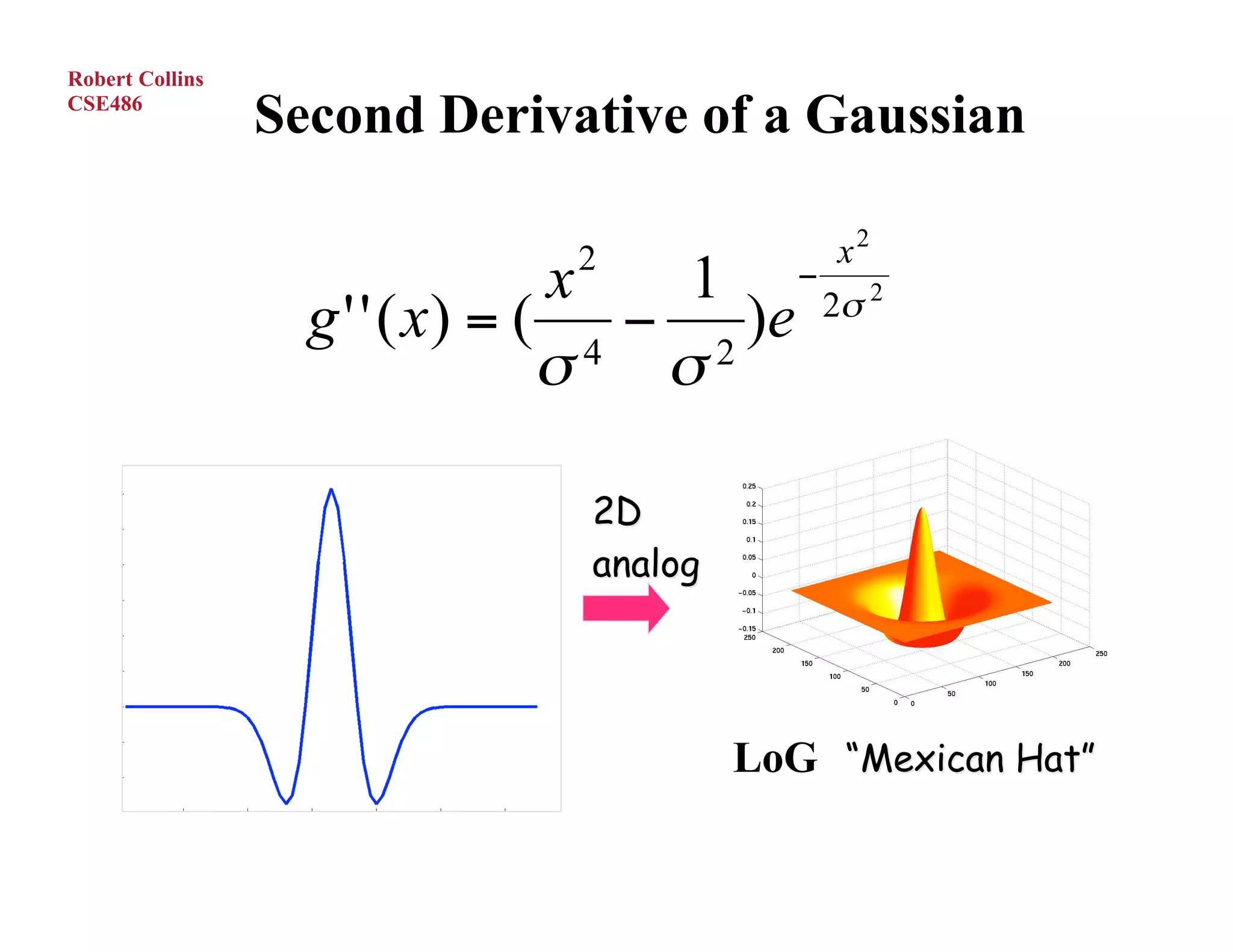
Second Derivative of a Gaussian
2 x2
x 1 − 2
g ' ' ( x ) = ( 4 − 2 )e
3
2σ
σ σ
2D
analog
LoG “Mexican Hat”
O.Camps, PSU

18. Robert Collins
CSE486
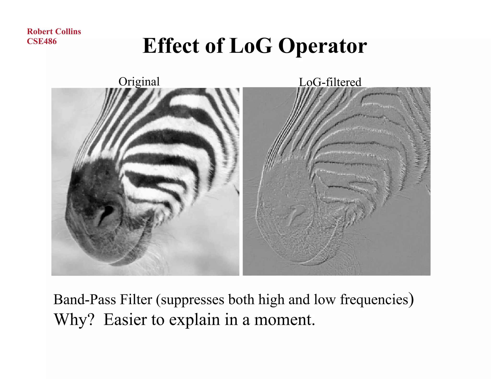
Effect of LoG Operator
Original LoG-filtered
Band-Pass Filter (suppresses both high and low frequencies)
Why? Easier to explain in a moment.

19. Robert Collins
CSE486
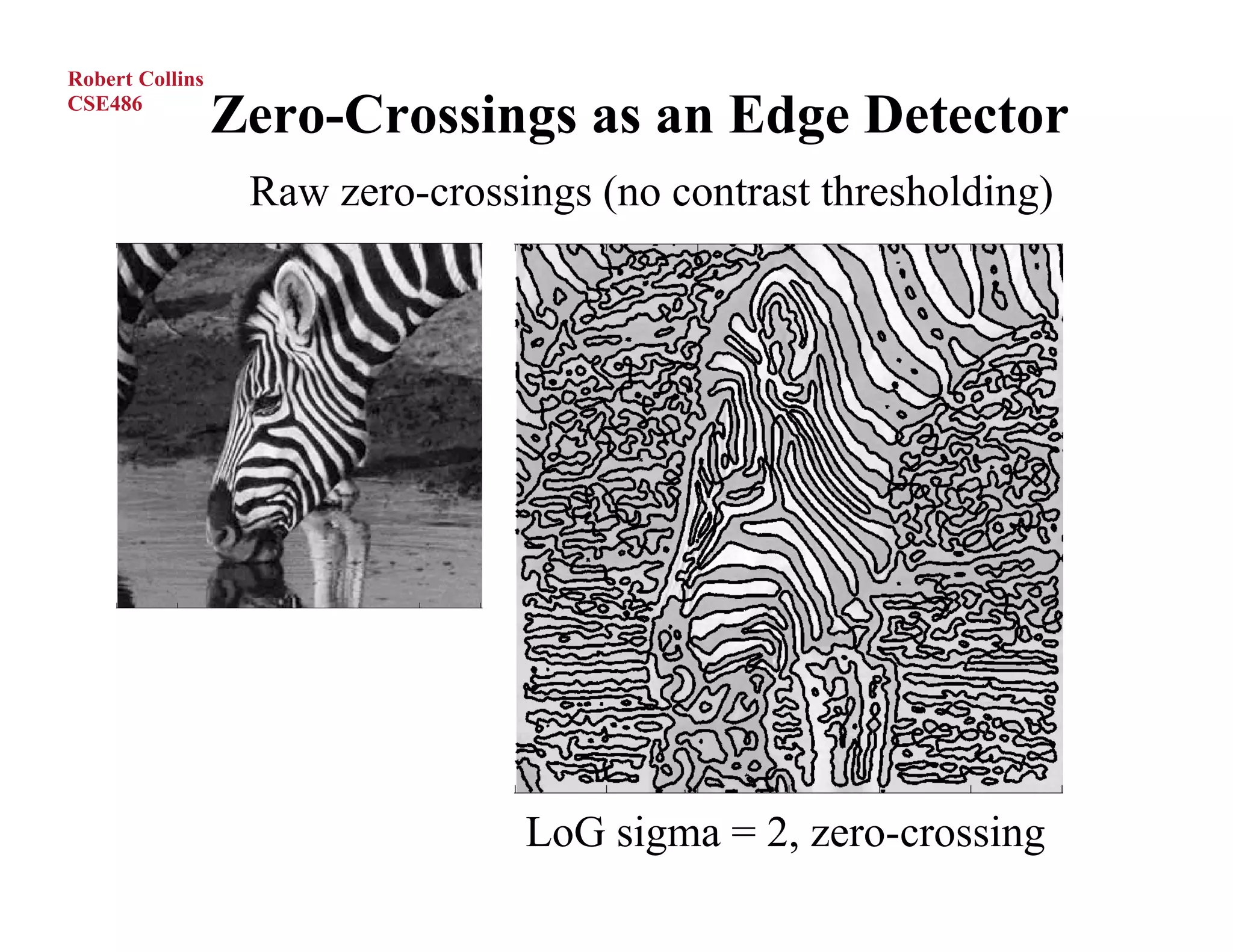
Zero-Crossings as an Edge Detector
Raw zero-crossings (no contrast thresholding)
LoG sigma = 2, zero-crossing

20. Robert Collins
CSE486
Zero-Crossings as an Edge Detector
Raw zero-crossings (no contrast thresholding)
LoG sigma = 4, zero-crossing

21. Robert Collins
CSE486
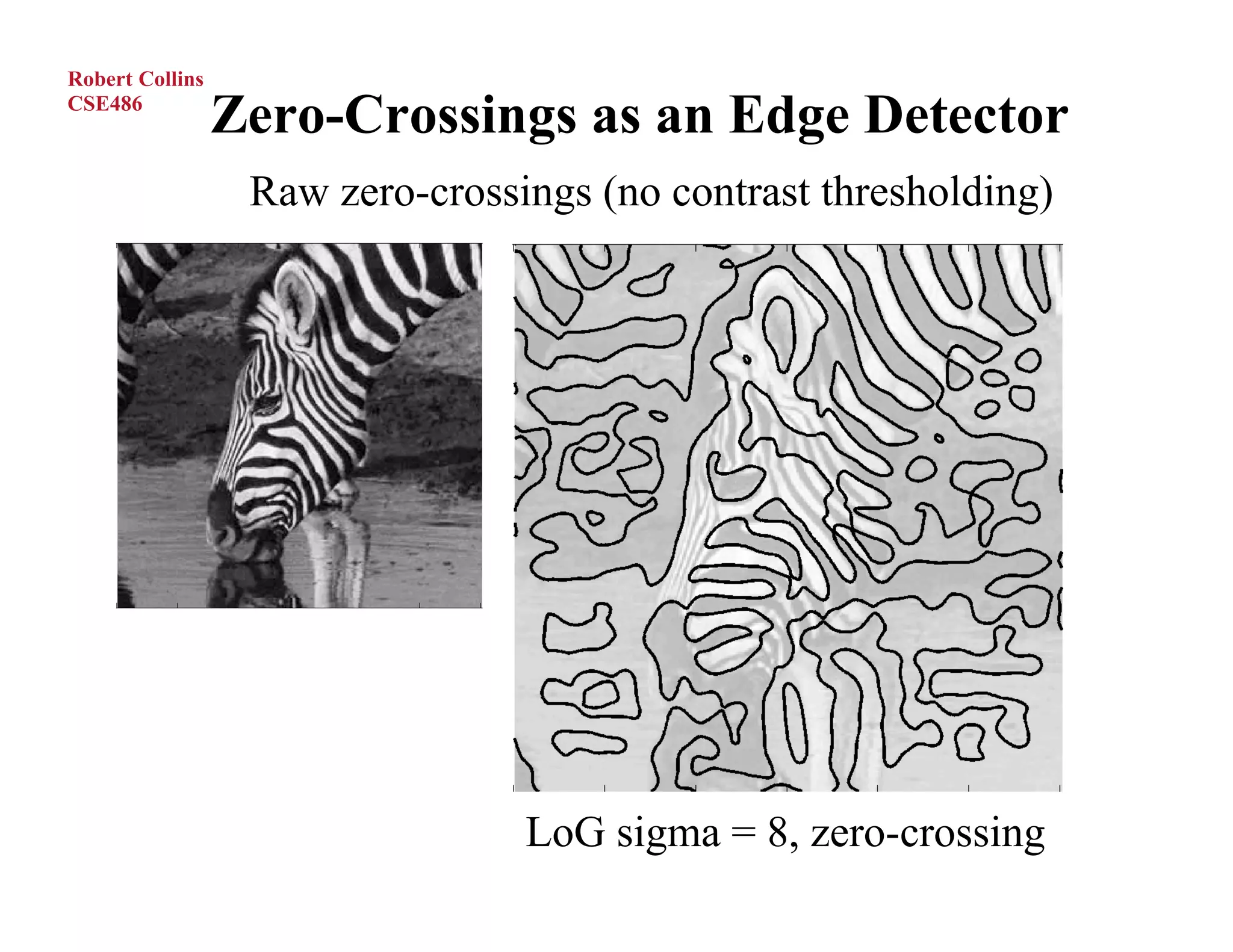
Zero-Crossings as an Edge Detector
Raw zero-crossings (no contrast thresholding)
LoG sigma = 8, zero-crossing

22. Robert Collins
CSE486
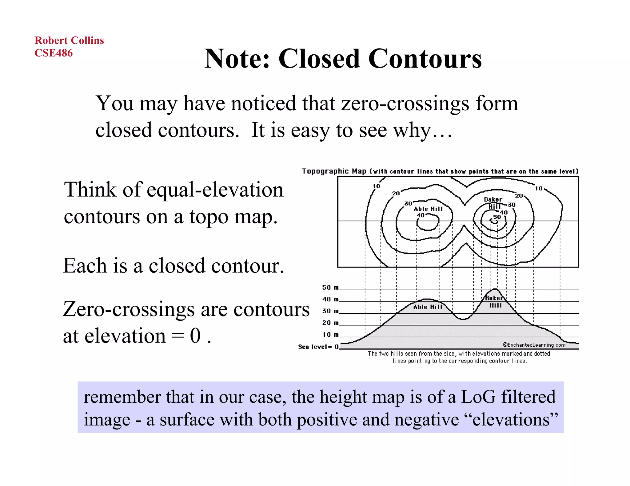
Note: Closed Contours
You may have noticed that zero-crossings form
closed contours. It is easy to see why…
Think of equal-elevation
contours on a topo map.
Each is a closed contour.
Zero-crossings are contours
at elevation = 0 .
remember that in our case, the height map is of a LoG filtered
image - a surface with both positive and negative “elevations”

23. Robert Collins
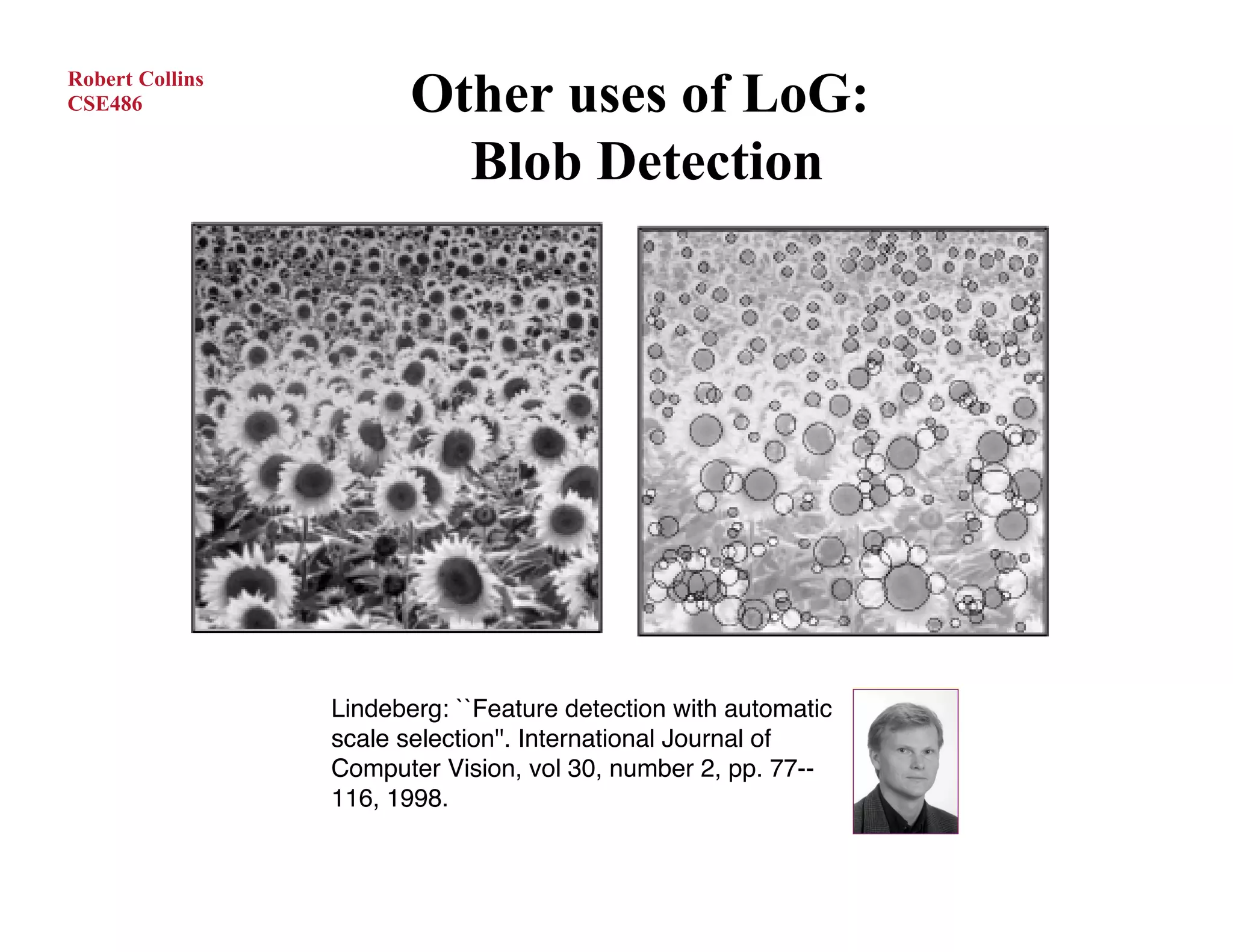
CSE486 Other uses of LoG:
Blob Detection
Lindeberg: ``Feature detection with automatic
scale selection''. International Journal of
Computer Vision, vol 30, number 2, pp. 77--
116, 1998.

24. Robert Collins
CSE486
Pause to Think for a Moment:
How can an edge finder also be used to
find blobs in an image?

25. Robert Collins
CSE486
Example: LoG Extrema
LoG maxima
sigma = 2
minima

26. Robert Collins
CSE486
LoG Extrema, Detail
maxima
LoG sigma = 2

27. Robert Collins
CSE486
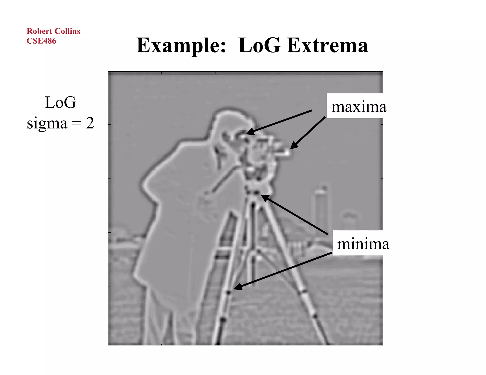
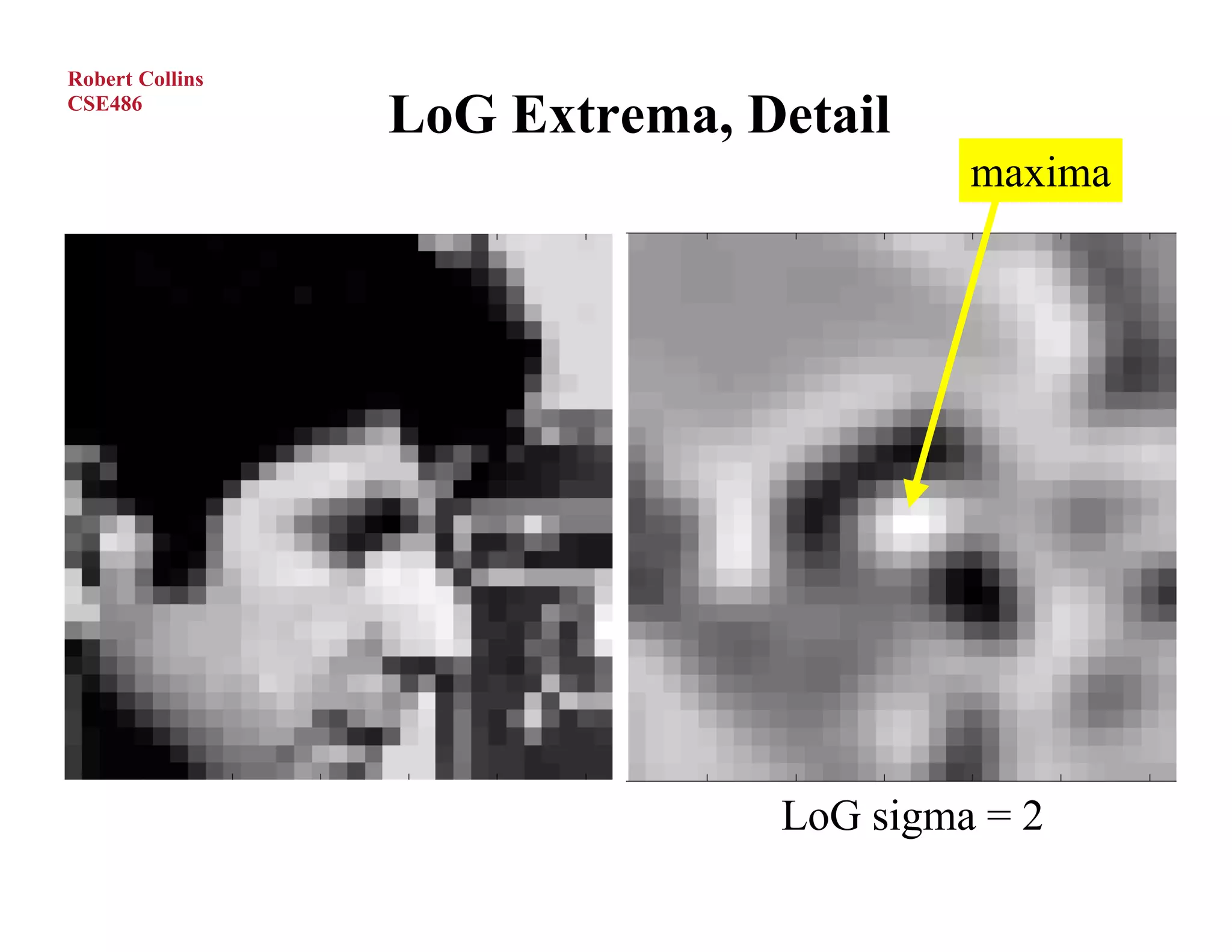
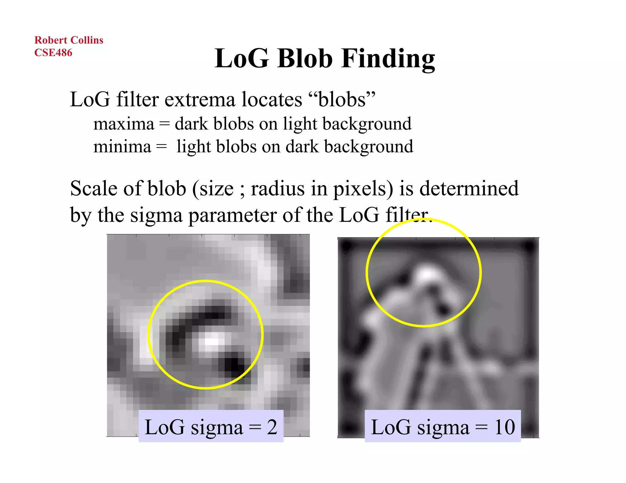
LoG Blob Finding
LoG filter extrema locates “blobs”
maxima = dark blobs on light background
minima = light blobs on dark background
Scale of blob (size ; radius in pixels) is determined
by the sigma parameter of the LoG filter.
LoG sigma = 2 LoG sigma = 10

28. Robert Collins
CSE486
Observe and Generalize
convolve result
with LoG
maxima

29. Robert Collins
CSE486
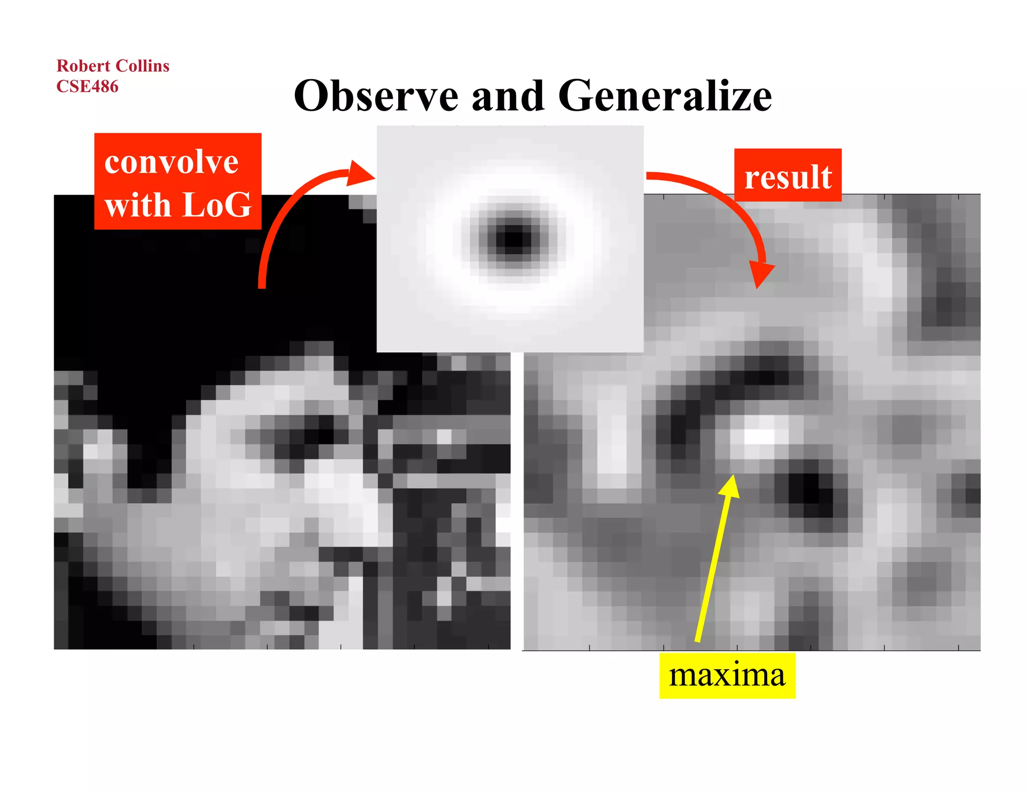
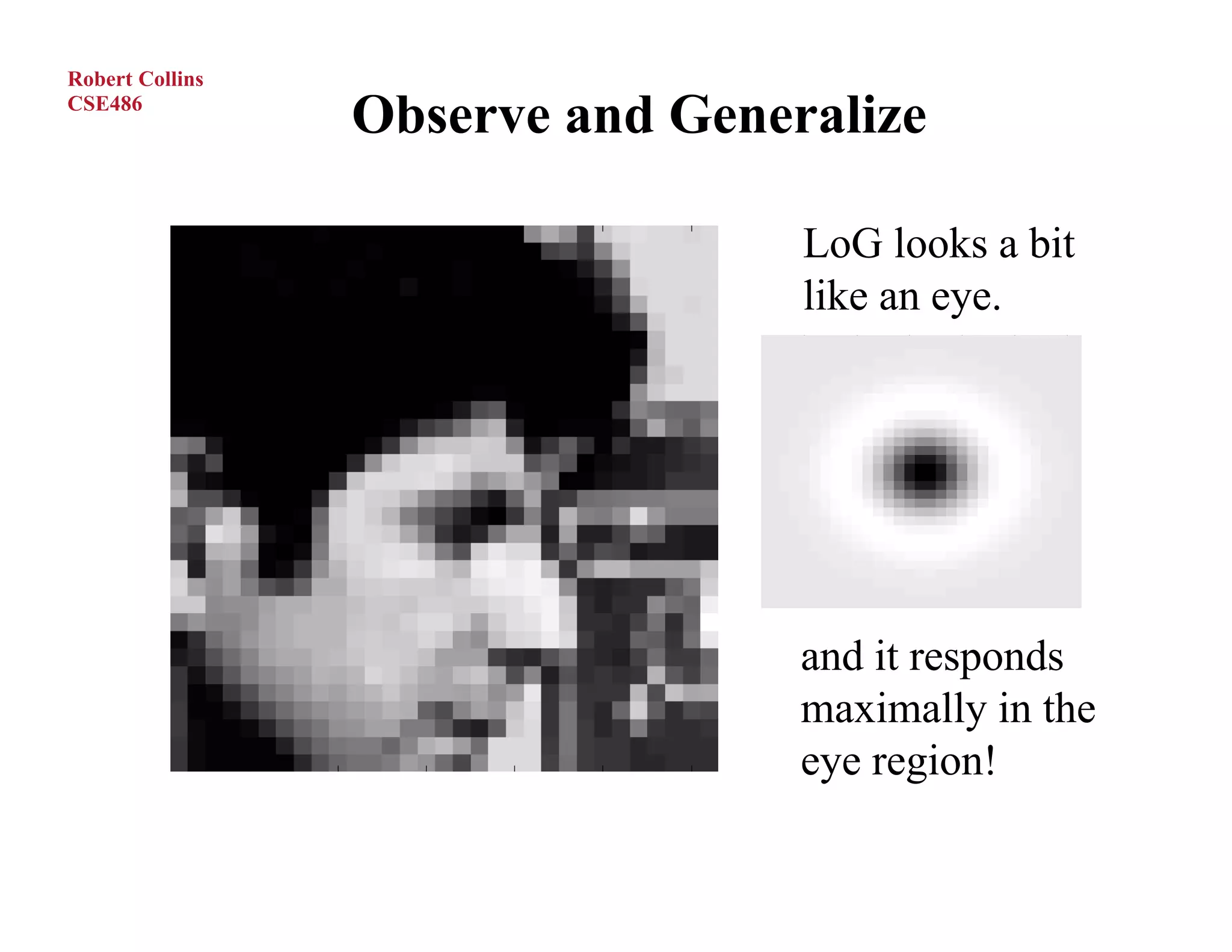
Observe and Generalize
LoG looks a bit
like an eye.
and it responds
maximally in the
eye region!

30. Robert Collins
CSE486
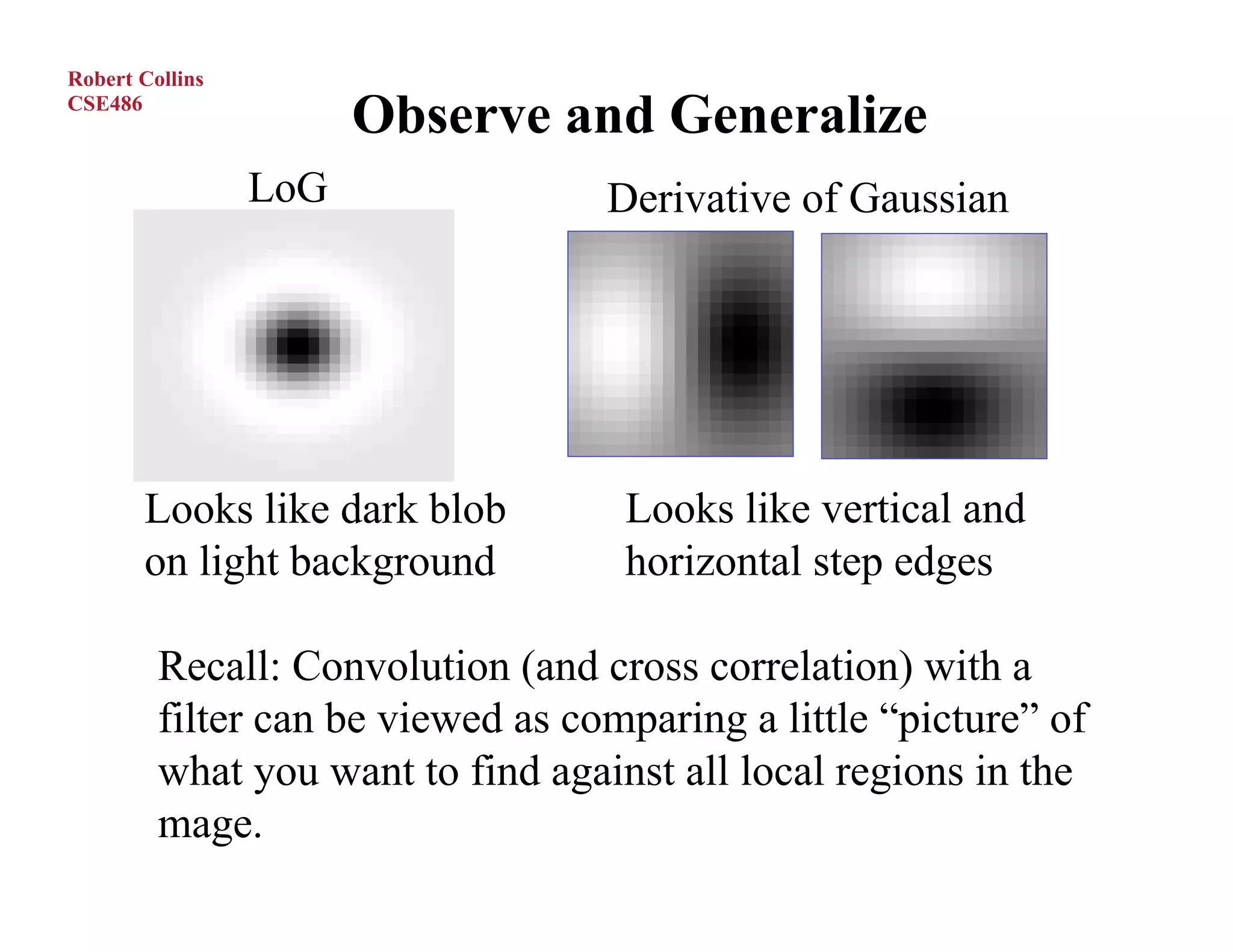
Observe and Generalize
LoG Derivative of Gaussian
Looks like dark blob Looks like vertical and
on light background horizontal step edges
Recall: Convolution (and cross correlation) with a
filter can be viewed as comparing a little “picture” of
what you want to find against all local regions in the
mage.

31. Robert Collins
CSE486
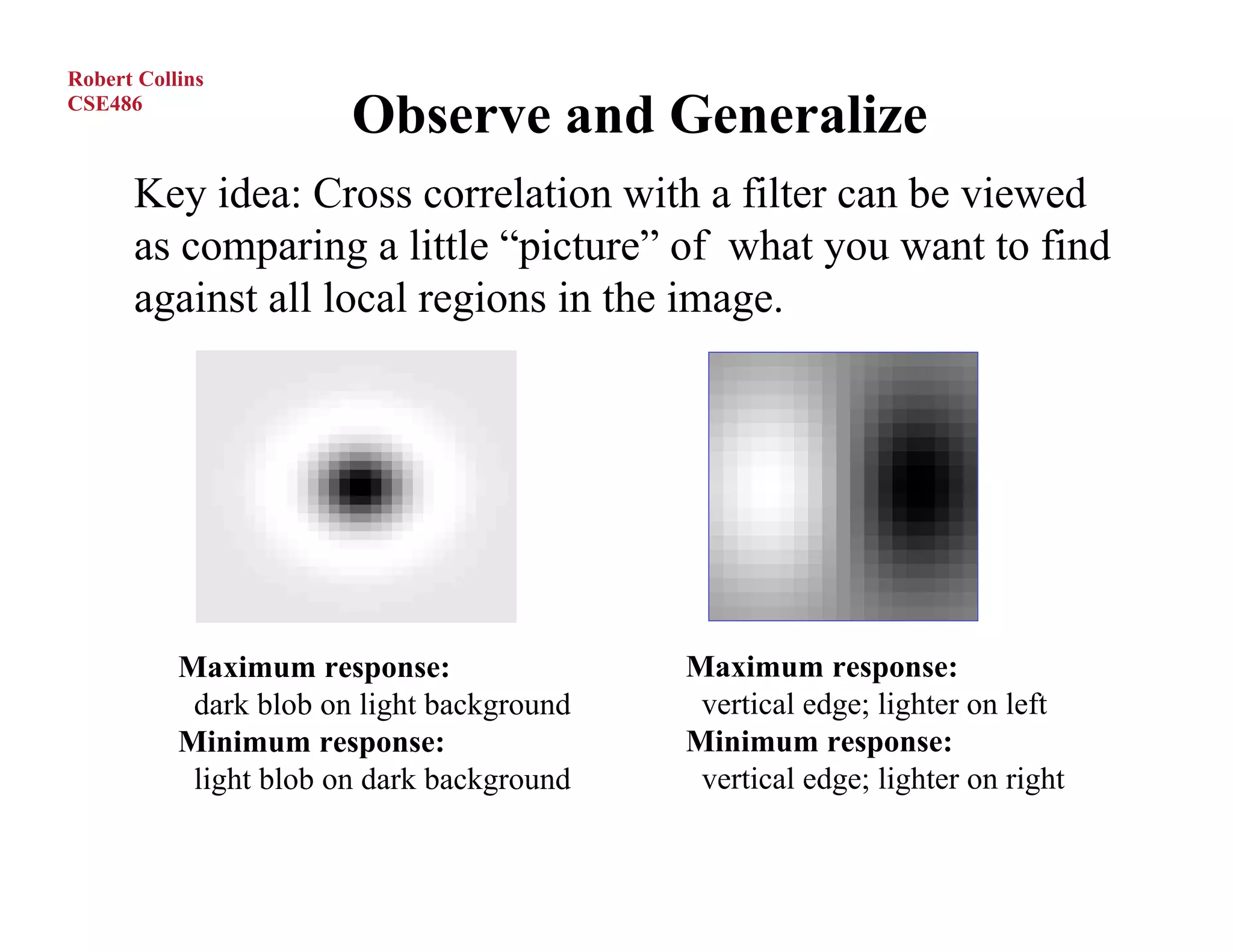
Observe and Generalize
Key idea: Cross correlation with a filter can be viewed
as comparing a little “picture” of what you want to find
against all local regions in the image.
Maximum response: Maximum response:
dark blob on light background vertical edge; lighter on left
Minimum response: Minimum response:
light blob on dark background vertical edge; lighter on right

32. Robert Collins
CSE486 Efficient Implementation
Approximating LoG with DoG
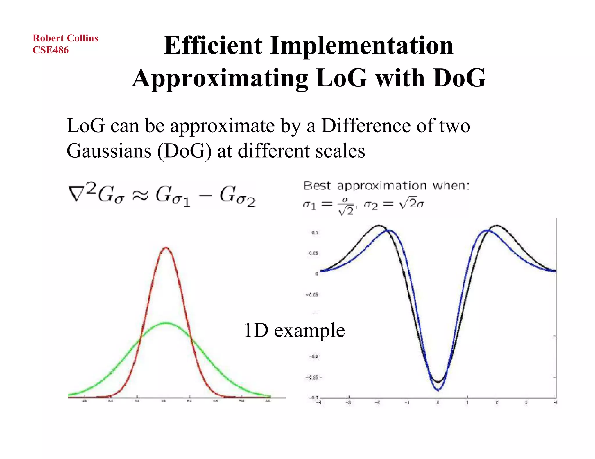
LoG can be approximate by a Difference of two
Gaussians (DoG) at different scales
1D example
M.Hebert, CMU

33. Robert Collins
CSE486
Efficient Implementation
LoG can be approximate by a Difference of two
Gaussians (DoG) at different scales.
Separability of and cascadability of Gaussians applies
to the DoG, so we can achieve efficient implementation
of the LoG operator.
DoG approx also explains bandpass filtering of LoG
(think about it. Hint: Gaussian is a low-pass filter)

34. Robert Collins
CSE486
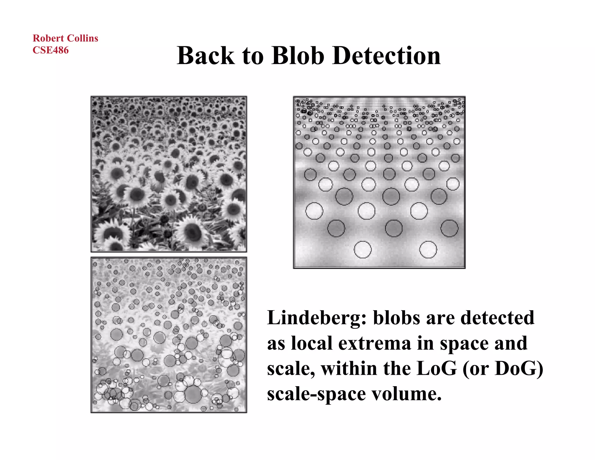
Back to Blob Detection
Lindeberg: blobs are detected
as local extrema in space and
scale, within the LoG (or DoG)
scale-space volume.

35. Robert Collins
CSE486
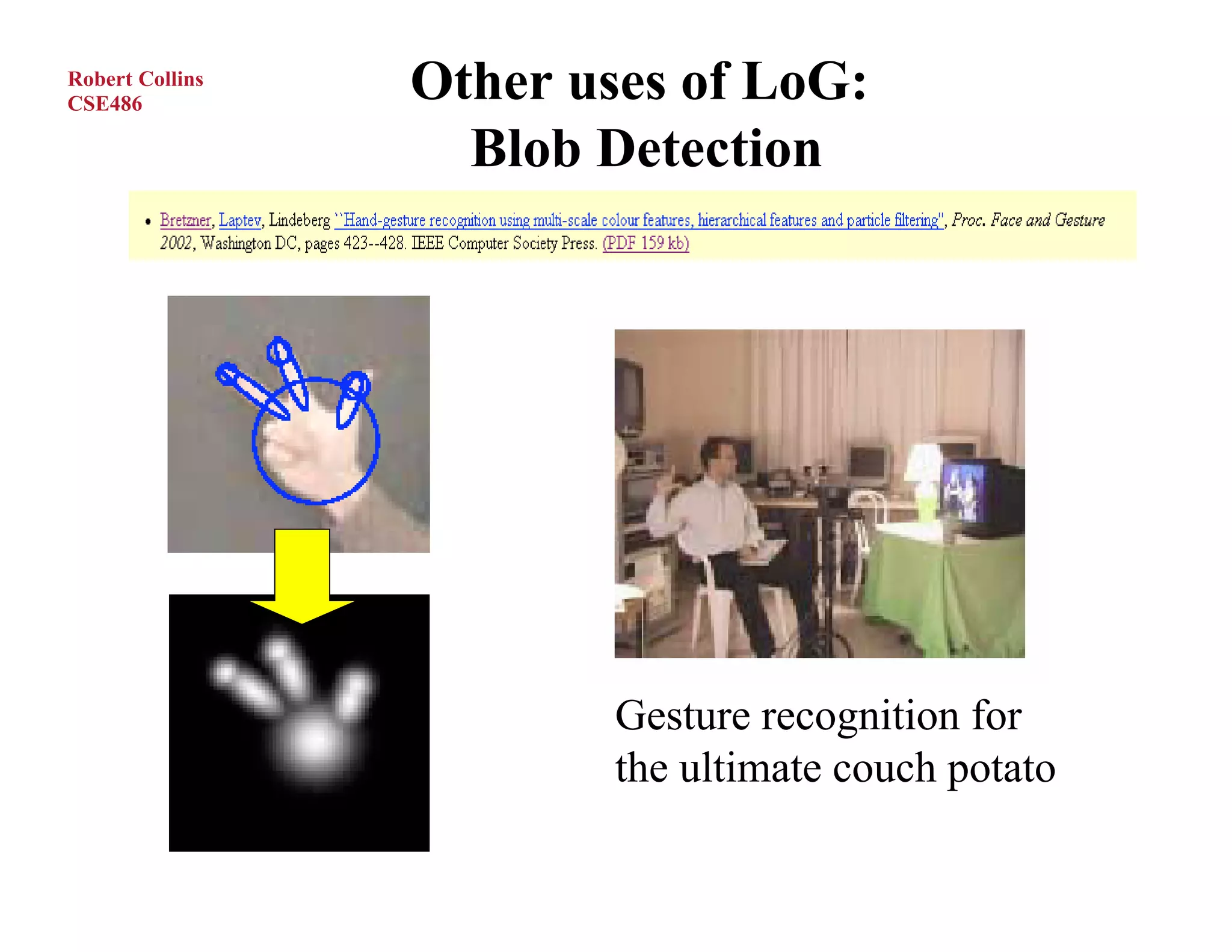
Other uses of LoG:
Blob Detection
Gesture recognition for
the ultimate couch potato

36. Robert Collins
CSE486
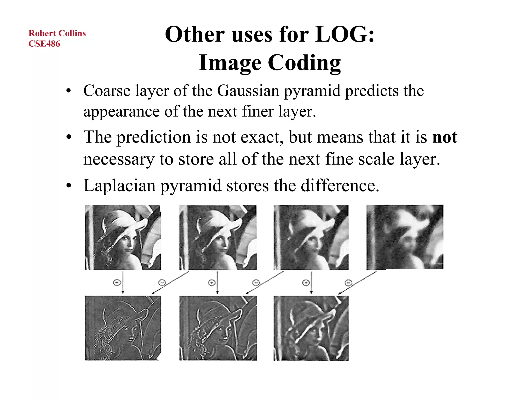
Other uses for LOG:
Image Coding
• Coarse layer of the Gaussian pyramid predicts the
appearance of the next finer layer.
• The prediction is not exact, but means that it is not
necessary to store all of the next fine scale layer.
• Laplacian pyramid stores the difference.

37. Robert Collins
CSE486
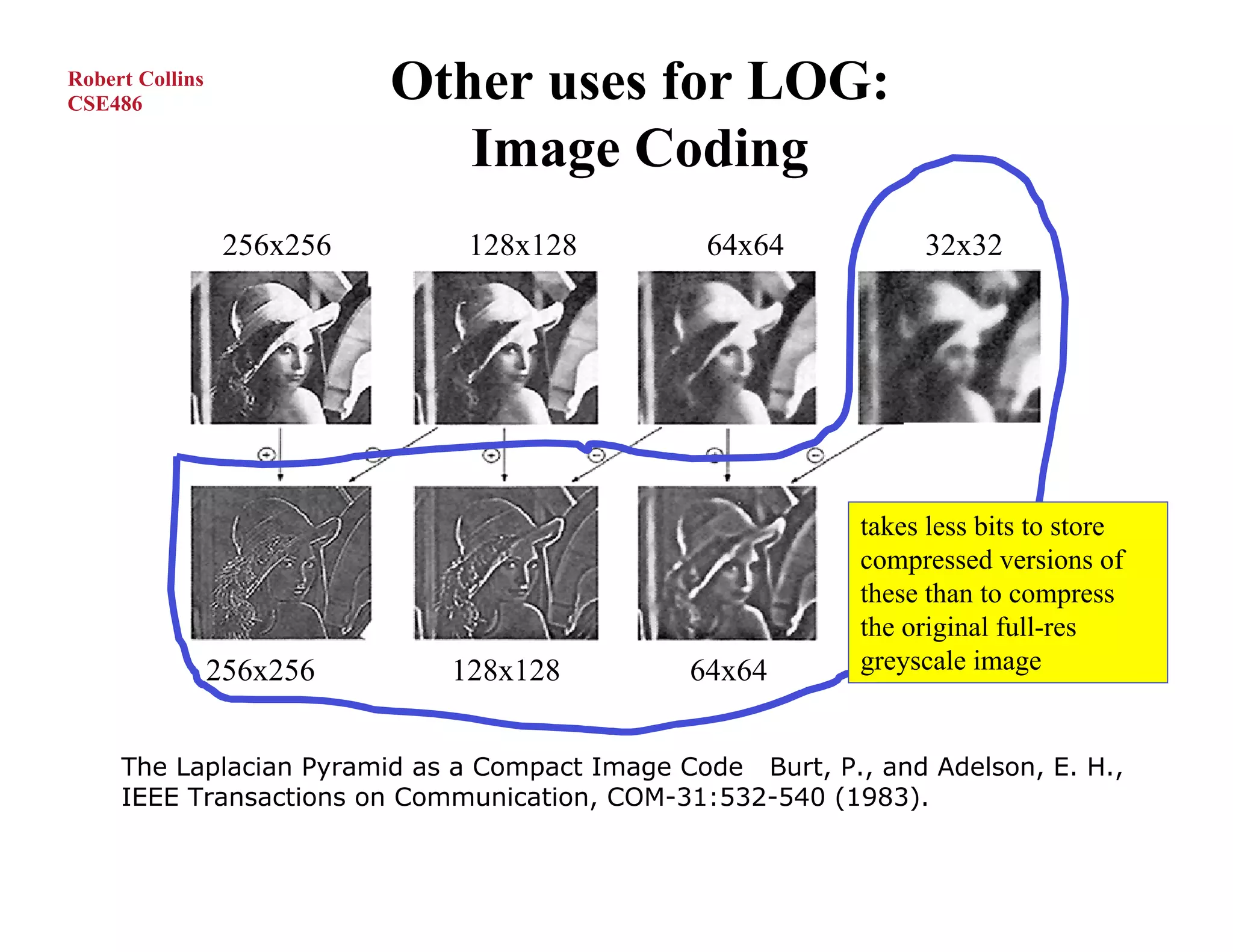
Other uses for LOG:
Image Coding
256x256 128x128 64x64 32x32
takes less bits to store
compressed versions of
these than to compress
the original full-res
256x256 128x128 64x64 greyscale image
The Laplacian Pyramid as a Compact Image Code Burt, P., and Adelson, E. H.,
IEEE Transactions on Communication, COM-31:532-540 (1983).