Transforms -- a mathematical conversion from one way of thinking to another to make a problem easier to solve

1. LAPLACE TRANSFORMS
INTRODUCTION

2. The French Newton
Pierre-Simon Laplace
 Developed mathematics in
astronomy, physics, and statistics
 Began work in calculus which led
to the Laplace Transform
 Focused later on celestial
mechanics
 One of the first scientists to
suggest the existence of black
holes

3. History of the Transform
 Euler began looking at integrals as solutions to differential equations
in the mid 1700’s:
 Lagrange took this a step further while working on probability
density functions and looked at forms of the following equation:
 Finally, in 1785, Laplace began using a transformation to solve
equations of finite differences which eventually lead to the current
transform

4. Definition
 Transforms -- a mathematical conversion from
one way of thinking to another to make a problem
easier to solve
transform
solution
in transform
way of
thinking
inverse
transform
solution
in original
way of
thinking
problem
in original
way of
thinking
2. Transforms

5. Laplace
transform
solution
in
s domain
inverse
Laplace
transform
solution
in time
domain
problem
in time
domain
• Other transforms
• Fourier
• z-transform
• wavelets
2. Transforms

6. Laplace transformation
linear
differential
equation
time
domain
solution
Laplace
transformed
equation
Laplace
solution
time domain
Laplace domain or
complex frequency domain
algebra
Laplace transform
inverse Laplace
transform
4. Laplace transforms

7. Basic Tool For Continuous Time:
Laplace Transform
 Convert time-domain functions and operations into
frequency-domain
 f(t)  F(s) (tR, sC
 Linear differential equations (LDE)  algebraic expression
in Complex plane
 Graphical solution for key LDE characteristics
 Discrete systems use the analogous z-transform





0
)
(
)
(
)]
(
[ dt
e
t
f
s
F
t
f st
L

8. The Complex Plane (review)
Imaginary axis (j)
Real axis
jy
x
u 

x
y

r
r


jy
x
u 

(complex) conjugate
y

2
2
1
|
|
|
|
tan
y
x
u
r
u
x
y
u






 


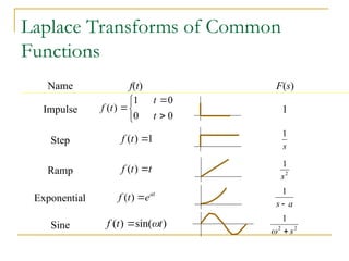
9. Laplace Transforms of Common
Functions
Name f(t) F(s)
Impulse
Step
Ramp
Exponential
Sine
1
s
1
2
1
s
a
s 
1
2
2
1
s


1
)
( 
t
f
t
t
f 
)
(
at
e
t
f 
)
(
)
sin(
)
( t
t
f 







0
0
0
1
)
(
t
t
t
f

10. Laplace Transform Properties
   
)
(
lim
)
(
lim
)
(
lim
)
0
(
)
(
)
(
)
)
(
1
)
(
)
(
)
0
(
)
(
)
(
)
(
)
(
)]
(
)
(
[
0
0
2
1
2
1
0
2
1
2
1
s
sF
t
f
-
s
sF
f
-
s
F
s
F
dτ
(τ
τ)f
(t
f
dt
t
f
s
s
s
F
dt
t
f
L
f
s
sF
t
f
dt
d
L
s
bF
s
aF
t
bf
t
af
L
s
t
s
t
t





























theorem
value
Final
theorem
value
Initial
n
Convolutio
n
Integratio
ation
Differenti
caling
Addition/S

11. LAPLACE TRANSFORMS
SIMPLE TRANSFORMATIONS

12. Transforms (1 of 11)
 Impulse --  (to)
F(s) =
0

e-st
 (to) dt
= e-sto
f(t)
t
 (to)
4. Laplace transforms

13. Transforms (2 of 11)
 Step -- u (to)
F(s) =
0

e-st
u (to) dt
= e-sto/s
f(t)
t
u (to)
1
4. Laplace transforms

14. Transforms (3 of 11)
 e-at
F(s) =
0
e-st
e-at
dt
= 1/(s+a)

4. Laplace transforms

15. Transforms (4 of 11)
f1(t)  f2(t)
a f(t)
eat
f(t)
f(t - T)
f(t/a)
F1(s) ± F2(s)
a F(s)
F(s-a)
eTs
F(as)
a F(as)
Linearity
Constant multiplication
Complex shift
Real shift
Scaling
4. Laplace transforms

16. Transforms (5 of 11)
 Most mathematical handbooks have tables
of Laplace transforms
4. Laplace transforms

17. LAPLACE TRANSFORMS
PARTIAL FRACTION EXPANSION

18. Definition
 Definition -- Partial fractions are several
fractions whose sum equals a given fraction
 Purpose -- Working with transforms requires
breaking complex fractions into simpler
fractions to allow use of tables of transforms

19. Partial Fraction Expansions
3
2
)
3
(
)
2
(
1







s
B
s
A
s
s
s  Expand into a term for each
factor in the denominator.
 Recombine RHS
 Equate terms in s and
constant terms. Solve.
 Each term is in a form so
that inverse Laplace
transforms can be applied.
 
)
3
(
)
2
(
2
)
3
(
)
3
(
)
2
(
1









s
s
s
B
s
A
s
s
s
3
2
2
1
)
3
(
)
2
(
1








s
s
s
s
s
1

 B
A 1
2
3 
 B
A

20. Example of Solution of an ODE
0
)
0
(
'
)
0
(
2
8
6
2
2




 y
y
y
dt
dy
dt
y
d  ODE w/initial conditions
 Apply Laplace transform to
each term
 Solve for Y(s)
 Apply partial fraction
expansion
 Apply inverse Laplace
transform to each term
s
s
Y
s
Y
s
s
Y
s /
2
)
(
8
)
(
6
)
(
2



)
4
(
)
2
(
2
)
(



s
s
s
s
Y
)
4
(
4
1
)
2
(
2
1
4
1
)
(






s
s
s
s
Y
4
2
4
1
)
(
4
2 t
t
e
e
t
y






21. Different terms of 1st degree
 To separate a fraction into partial fractions
when its denominator can be divided into
different terms of first degree, assume an
unknown numerator for each fraction
 Example --
 (11x-1)/(X2
- 1) = A/(x+1) + B/(x-1)
 = [A(x-1) +B(x+1)]/[(x+1)(x-1))]
 A+B=11
 -A+B=-1
 A=6, B=5

22. Repeated terms of 1st degree (1 of 2)
 When the factors of the denominator are of
the first degree but some are repeated,
assume unknown numerators for each
factor
 If a term is present twice, make the fractions
the corresponding term and its second power
 If a term is present three times, make the
fractions the term and its second and third
powers
3. Partial fractions

23. Repeated terms of 1st degree (2 of 2)
 Example --
 (x2
+3x+4)/(x+1)3
= A/(x+1) + B/(x+1)2
+
C/(x+1)3
 x2
+3x+4 = A(x+1)2
+ B(x+1) + C
 = Ax2
+ (2A+B)x + (A+B+C)
 A=1
 2A+B = 3
 A+B+C = 4
 A=1, B=1, C=2
3. Partial fractions

24. Different quadratic terms
 When there is a quadratic term, assume a
numerator of the form Ax + B
 Example --
 1/[(x+1) (x2
+ x + 2)] = A/(x+1) + (Bx +C)/ (x2
+
x + 2)
 1 = A (x2
+ x + 2) + Bx(x+1) + C(x+1)
 1 = (A+B) x2
+ (A+B+C)x +(2A+C)
 A+B=0
 A+B+C=0
 2A+C=1
 A=0.5, B=-0.5, C=0
3. Partial fractions

25. Repeated quadratic terms
 Example --
 1/[(x+1) (x2
+ x + 2)2
] = A/(x+1) + (Bx +C)/ (x2
+
x + 2) + (Dx +E)/ (x2
+ x + 2)2
 1 = A(x2
+ x + 2)2
+ Bx(x+1) (x2
+ x + 2) +
C(x+1) (x2
+ x + 2) + Dx(x+1) + E(x+1)
 A+B=0
 2A+2B+C=0
 5A+3B+2C+D=0
 4A+2B+3C+D+E=0
 4A+2C+E=1
 A=0.25, B=-0.25, C=0, D=-0.5, E=0
3. Partial fractions

26. Apply Initial- and Final-Value
Theorems to this Example
 Laplace
transform of the
function.
 Apply final-value
theorem
 Apply initial-
value theorem
)
4
(
)
2
(
2
)
(



s
s
s
s
Y
 
4
1
)
4
0
(
)
2
0
(
)
0
(
)
0
(
2
)
(
lim 




 t
f
t
  0
)
4
(
)
2
(
)
(
)
(
2
)
(
lim 0 







 t
f
t

27. LAPLACE TRANSFORMS
SOLUTION PROCESS

28. Solution process (1 of 8)
 Any nonhomogeneous linear differential
equation with constant coefficients can be
solved with the following procedure, which
reduces the solution to algebra
4. Laplace transforms

29. Solution process (2 of 8)
 Step 1: Put differential equation into
standard form
 D2
y + 2D y + 2y = cos t
 y(0) = 1
 D y(0) = 0

30. Solution process (3 of 8)
 Step 2: Take the Laplace transform of both
sides
 L{D2
y} + L{2D y} + L{2y} = L{cos t}

31. Solution process (4 of 8)
 Step 3: Use table of transforms to express
equation in s-domain
 L{D2
y} + L{2D y} + L{2y} = L{cos  t}
 L{D2
y} = s2
Y(s) - sy(0) - D y(0)
 L{2D y} = 2[ s Y(s) - y(0)]
 L{2y} = 2 Y(s)
 L{cos t} = s/(s2
+ 1)
 s2
Y(s) - s + 2s Y(s) - 2 + 2 Y(s) = s /(s2
+ 1)

32. Solution process (5 of 8)
 Step 4: Solve for Y(s)
 s2
Y(s) - s + 2s Y(s) - 2 + 2 Y(s) = s/(s2
+ 1)
 (s2
+ 2s + 2) Y(s) = s/(s2
+ 1) + s + 2
 Y(s) = [s/(s2
+ 1) + s + 2]/ (s2
+ 2s + 2)
 = (s3
+ 2 s2
+ 2s + 2)/[(s2
+ 1) (s2
+ 2s + 2)]

33. Solution process (6 of 8)
 Step 5: Expand equation into format covered by
table
 Y(s) = (s3
+ 2 s2
+ 2s + 2)/[(s2
+ 1) (s2
+ 2s + 2)]
 = (As + B)/ (s2
+ 1) + (Cs + E)/ (s2
+ 2s + 2)
 (A+C)s3
+ (2A + B + E) s2
+ (2A + 2B + C)s + (2B
+E)
 1 = A + C
 2 = 2A + B + E
 2 = 2A + 2B + C
 2 = 2B + E
 A = 0.2, B = 0.4, C = 0.8, E = 1.2

34. Solution process (7 of 8)
 (0.2s + 0.4)/ (s2
+ 1)
 = 0.2 s/ (s2
+ 1) + 0.4 / (s2
+ 1)
 (0.8s + 1.2)/ (s2
+ 2s + 2)
 = 0.8 (s+1)/[(s+1)2
+ 1] + 0.4/ [(s+1)2
+ 1]

35. Solution process (8 of 8)
 Step 6: Use table to convert s-domain to
time domain
 0.2 s/ (s2
+ 1) becomes 0.2 cos t
 0.4 / (s2
+ 1) becomes 0.4 sin t
 0.8 (s+1)/[(s+1)2
+ 1] becomes 0.8 e-t
cos t
 0.4/ [(s+1)2
+ 1] becomes 0.4 e-t
sin t
 y(t) = 0.2 cos t + 0.4 sin t + 0.8 e-t
cos t + 0.4 e-
t
sin t

36. LAPLACE TRANSFORMS
TRANSFER FUNCTIONS

37. Introduction
 Definition -- a transfer function is an
expression that relates the output to the
input in the s-domain
differential
equation
r(t) y(t)
transfer
function
r(s) y(s)
5. Transfer functions

38. Transfer Function
 Definition
 H(s) = Y(s) / X(s)
 Relates the output of a linear system (or
component) to its input
 Describes how a linear system responds to
an impulse
 All linear operations allowed
 Scaling, addition, multiplication
H(s)
X(s) Y(s)

39. Block Diagrams
 Pictorially expresses flows and relationships
between elements in system
 Blocks may recursively be systems
 Rules
 Cascaded (non-loading) elements: convolution
 Summation and difference elements
 Can simplify

40. Typical block diagram
control
Gc(s)
plant
Gp(s)
feedback
H(s)
pre-filter
G1(s)
post-filter
G2(s)
reference input, R(s)
error, E(s)
plant inputs, U(s)
output, Y(s)
feedback, H(s)Y(s)
5. Transfer functions

41. Example
v(t)
R
C
L
v(t) = R I(t) + 1/C I(t) dt + L di(t)/dt
V(s) = [R I(s) + 1/(C s) I(s) + s L I(s)]
Note: Ignore initial conditions
5. Transfer functions

42. Block diagram and transfer function
 V(s)
 = (R + 1/(C s) + s L ) I(s)
 = (C L s2
+ C R s + 1 )/(C s) I(s)
 I(s)/V(s) = C s / (C L s2
+ C R s + 1 )
C s / (C L s2
+ C R s + 1 )
V(s) I(s)
5. Transfer functions

43. Block diagram reduction rules
G1 G2 G1 G2
U Y U Y
G1
G2
U Y
+
+ G1 + G2
U Y
G1
G2
U Y
+
- G1 /(1+G1 G2)
U Y
Series
Parallel
Feedback
5. Transfer functions

44. Rational Laplace Transforms
m
s
F
s
A
s
s
F
s
B
s
b
s
b
s
b
s
B
a
s
a
s
a
s
A
s
B
s
A
s
F
m
m
n
n
poles
#
system
of
Order
complex
are
zeroes
and
Poles
(So,
:
Zeroes
(So,
:
Poles


















)
0
*)
(
0
*)
(
*
)
*)
(
0
*)
(
*
...
)
(
...
)
(
)
(
)
(
)
(
0
1
0
1

45. First Order System
Reference
)
(s
Y
)
(s
R

)
(s
E
1
)
(s
B
)
(s
U
sT

1
1
K
sT
K
sT
K
K
s
R
s
Y





1
1
)
(
)
(

46. First Order System
Impulse
response
Exponential
Step response Step,
exponential
Ramp response Ramp, step,
exponential
1 sT
K

/
1
2
T
s
KT
-
s
KT
-
s
K

/
1 T
s
K
-
s
K

No oscillations (as seen by poles)

47. Second Order System
:
frequency
natural
Undamped
where
:
ratio
Damping
(ie,
part
imaginary
zero
-
non
have
poles
if
Oscillates
:
response
Impulse
J
K
JK
B
B
B
JK
B
s
s
K
Bs
Js
K
s
R
s
Y
N
c
c
N
N
N
















2
)
0
4
2
)
(
)
(
2
2
2
2
2

48. Second Order System: Parameters
n
oscillatio
the
of
frequency
the
gives
frequency
natural
undamped
of
tion
Interpreta
0)
Im
0,
(Re
Overdamped
1
Im)
(Re
d
Underdampe
0)
Im
0,
(Re
n
oscillatio
Undamped
ratio
damping
of
tion
Interpreta
N














:
0
:
1
0
:
0

49. Transient Response Characteristics
state
steady
of
%
specified
within
stays
time
Settling
:
reached
is
value
peak
which
at
Time
:
value
state
steady
reach
first
until
delay
time
Rise
:
value
state
steady
of
50%
reach
until
Delay
:


s
p
r
d
t
t
t
t
0.5 1 1.5 2 2.5 3
0.25
0.5
0.75
1
1.25
1.5
1.75
2
r
t
overshoot
maximum

p
M
p
t s
t
d
t

50. Transient Response
 Estimates the shape of the curve based on
the foregoing points on the x and y axis
 Typically applied to the following inputs
 Impulse
 Step
 Ramp
 Quadratic (Parabola)

51. Effect of pole locations
Faster Decay Faster Blowup
Oscillations
(higher-freq)
Im(s)
Re(s)
(e-at
) (eat
)

52. Basic Control Actions: u(t)
:
control
al
Differenti
:
control
Integral
:
control
al
Proportion
s
K
s
E
s
U
t
e
dt
d
K
t
u
s
K
s
E
s
U
dt
t
e
K
t
u
K
s
E
s
U
t
e
K
t
u
d
d
i
t
i
p
p







)
(
)
(
)
(
)
(
)
(
)
(
)
(
)
(
)
(
)
(
)
(
)
(
0

53. Effect of Control Actions
 Proportional Action
 Adjustable gain (amplifier)
 Integral Action
 Eliminates bias (steady-state error)
 Can cause oscillations
 Derivative Action (“rate control”)
 Effective in transient periods
 Provides faster response (higher sensitivity)
 Never used alone

54. Basic Controllers
 Proportional control is often used by itself
 Integral and differential control are typically
used in combination with at least proportional
control
 eg, Proportional Integral (PI) controller:













s
T
K
s
K
K
s
E
s
U
s
G
i
p
I
p
1
1
)
(
)
(
)
(

55. Summary of Basic Control
 Proportional control
 Multiply e(t) by a constant
 PI control
 Multiply e(t) and its integral by separate constants
 Avoids bias for step
 PD control
 Multiply e(t) and its derivative by separate constants
 Adjust more rapidly to changes
 PID control
 Multiply e(t), its derivative and its integral by separate constants
 Reduce bias and react quickly

56. Root-locus Analysis
 Based on characteristic eqn of closed-loop transfer
function
 Plot location of roots of this eqn
 Same as poles of closed-loop transfer function
 Parameter (gain) varied from 0 to 
 Multiple parameters are ok
 Vary one-by-one
 Plot a root “contour” (usually for 2-3 params)
 Quickly get approximate results
 Range of parameters that gives desired response

57. LAPLACE TRANSFORMS
LAPLACE APPLICATIONS

58. Initial value
 In the initial value of f(t) as t approaches 0
is given by
f(0 ) = Lim s F(s)
s 
f(t) = e -t
F(s) = 1/(s+1)
f(0 ) = Lim s /(s+1) = 1
s 
Example
6. Laplace applications

59. Final value
 In the final value of f(t) as t approaches 
is given by
f(0 ) = Lim s F(s)
s 0
f(t) = e -t
F(s) = 1/(s+1)
f(0 ) = Lim s /(s+1) = 0
s 0
Example
6. Laplace applications

60. Apply Initial- and Final-Value
Theorems to this Example
 Laplace
transform of the
function.
 Apply final-value
theorem
 Apply initial-
value theorem
)
4
(
)
2
(
2
)
(



s
s
s
s
Y
 
4
1
)
4
0
(
)
2
0
(
)
0
(
)
0
(
2
)
(
lim 




 t
f
t
  0
)
4
(
)
2
(
)
(
)
(
2
)
(
lim 0 







 t
f
t

61. Poles
 The poles of a Laplace function are the
values of s that make the Laplace function
evaluate to infinity. They are therefore the
roots of the denominator polynomial
 10 (s + 2)/[(s + 1)(s + 3)] has a pole at s = -
1 and a pole at s = -3
 Complex poles always appear in complex-
conjugate pairs
 The transient response of system is
determined by the location of poles
6. Laplace applications

62. Zeros
 The zeros of a Laplace function are the
values of s that make the Laplace function
evaluate to zero. They are therefore the
zeros of the numerator polynomial
 10 (s + 2)/[(s + 1)(s + 3)] has a zero at s =
-2
 Complex zeros always appear in complex-
conjugate pairs
6. Laplace applications

63. Stability
 A system is stable if bounded inputs produce bounded
outputs
 The complex s-plane is divided into two regions: the stable
region, which is the left half of the plane, and the unstable
region, which is the right half of the s-plane
s-plane
stable unstable
x
x
x
x x
x
x
j


64. LAPLACE TRANSFORMS
FREQUENCY RESPONSE

65. Introduction
 Many problems can be thought of in the
time domain, and solutions can be
developed accordingly.
 Other problems are more easily thought of
in the frequency domain.
 A technique for thinking in the frequency
domain is to express the system in terms
of a frequency response
7. Frequency response

66. Definition
 The response of the system to a sinusoidal
signal. The output of the system at each
frequency is the result of driving the system
with a sinusoid of unit amplitude at that
frequency.
 The frequency response has both amplitude
and phase
7. Frequency response

67. Process
 The frequency response is computed by
replacing s with j  in the transfer function
f(t) = e -t
F(s) = 1/(s+1)
Example
F(j ) = 1/(j  +1)
Magnitude = 1/SQRT(1 + 2
)
Magnitude in dB = 20 log10 (magnitude)
Phase = argument = ATAN2(- , 1)
magnitude in dB

7. Frequency response

68. Graphical methods
 Frequency response is a graphical method
 Polar plot -- difficult to construct
 Corner plot -- easy to construct
7. Frequency response

69. Constant K
+180o
+90o
0o
-270o
-180o
-90o
60 dB
40 dB
20 dB
0 dB
-20 dB
-40 dB
-60 dB
magnitude
phase
0.1 1 10 100
, radians/sec
20 log10 K
arg K
7. Frequency response

70. Simple pole or zero at origin, 1/ (j)n
+180o
+90o
0o
-270o
-180o
-90o
60 dB
40 dB
20 dB
0 dB
-20 dB
-40 dB
-60 dB
magnitude
phase
0.1 1 10 100
, radians/sec
1/ 
1/ 2
1/ 3
1/ 
1/ 2
1/ 3
G(s) = n
2
/(s2
+ 2 ns +  n
2
)

71. Simple pole or zero, 1/(1+j)
+180o
+90o
0o
-270o
-180o
-90o
60 dB
40 dB
20 dB
0 dB
-20 dB
-40 dB
-60 dB
magnitude
phase
0.1 1 10 100
T
7. Frequency response

72. Error in asymptotic approximation
T
0.01
0.1
0.5
0.76
1.0
1.31
1.73
2.0
5.0
10.0
dB
0
0.043
1
2
3
4.3
6.0
7.0
14.2
20.3
arg (deg)
0.5
5.7
26.6
37.4
45.0
52.7
60.0
63.4
78.7
84.3
7. Frequency response

73. Quadratic pole or zero
+180o
+90o
0o
-270o
-180o
-90o
60 dB
40 dB
20 dB
0 dB
-20 dB
-40 dB
-60 dB
magnitude
phase
0.1 1 10 100
T
7. Frequency response

74. Transfer Functions
 Defined as G(s) = Y(s)/U(s)
 Represents a normalized model of a process,
i.e., can be used with any input.
 Y(s) and U(s) are both written in deviation
variable form.
 The form of the transfer function indicates the
dynamic behavior of the process.

75. Derivation of a Transfer Function
T
F
F
T
F
T
F
dt
dT
M )
( 2
1
2
2
1
1 


  Dynamic model of
CST thermal mixer
 Apply deviation
variables
 Equation in terms
of deviation
variables.
0
2
2
0
1
1
0 T
T
T
T
T
T
T
T
T 








T
F
F
T
F
T
F
dt
T
d
M 







)
( 2
1
2
2
1
1

76. Derivation of a Transfer Function
 
2
1
1
1 )
(
)
(
)
(
F
F
s
M
F
s
T
s
T
s
G




 Apply Laplace transform
to each term considering
that only inlet and outlet
temperatures change.
 Determine the transfer
function for the effect of
inlet temperature changes
on the outlet temperature.
 Note that the response is
first order.
 
2
1
2
2
1
1 )
(
)
(
)
(
F
F
s
M
s
T
F
s
T
F
s
T





77. Poles of the Transfer Function
Indicate the Dynamic Response
 For a, b, c, and d positive constants, transfer
function indicates exponential decay, oscillatory
response, and exponential growth, respectively.
)
(
)
(
)
(
)
( 2
d
s
C
c
bs
s
B
a
s
A
s
Y







dt
pt
at
e
C
t
e
B
e
A
t
y 




 
)
sin(
)
( 
)
(
)
(
)
(
1
)
( 2
d
s
c
bs
s
a
s
s
G






78. Poles on a Complex Plane
Re
Im

79. Exponential Decay
Re
Im
Time
y

80. Damped Sinusoidal
Re
Im
Time
y

81. Exponentially Growing Sinusoidal
Behavior (Unstable)
Re
Im
Time
y

82. What Kind of Dynamic Behavior?
Re
Im

83. Unstable Behavior
 If the output of a process grows without bound
for a bounded input, the process is referred to
a unstable.
 If the real portion of any pole of a transfer
function is positive, the process corresponding
to the transfer function is unstable.
 If any pole is located in the right half plane,
the process is unstable.

84. THANK YOU