representation, unbalanced data, multiclass classification, theoretical modelling, real-world implementations, evaluation, holdout estimation, crossvalidation, leave-one-out, bootstrap,

1. Machine Learning for Language Technology 2015
http://stp.lingfil.uu.se/~santinim/ml/2015/ml4lt_2015.htm
Machine Learning in Practice (2)
Marina Santini
santinim@stp.lingfil.uu.se
Department of Linguistics and Philology
Uppsala University, Uppsala, Sweden
Autumn 2015

2. Acknowledgements
• Weka’s slides
• Feature engineering:
http://machinelearningmastery.com/discover-feature-engineering-how-to-
engineer-features-and-how-to-get-good-at-it/
• - Daume' III (2015): 53-64
- Witten et al. (2011): 147-156
Lecture 8: ML in Practice (1)

3. Outline
• The importance of features
• Unbalanced data, multiclass classification,
teoretical model vs. real-world implementaton
• Evaluation:
– How to assess what has been learned
– Holdout estimation
– Crossvalidation
– Leave-one-out
– Boostrap
Lecture 8: ML in Practice (1)

4. The importance of good features
• Garbage in – garbage out
Lecture 8: ML in Practice (1)

5. Bag of Words Representation
Lecture 8: ML in Practice (1)

6. Parts Of Speech (PoS) representation
Lecture 8: ML in Practice (1)

7. The Importance of Good Features
• Ex in Text Classification
– BOW (Bag of words) (either counts or binary)
– Phrases
– n-Grams
– Chunks
– PoSs
– PoS n-grams
– etc.
Lecture 8: ML in Practice (1)

8. ML success: Feature representation
(aka feature engineering)
• The success of ML algorithms depens on how you present the data:
you need great features that describe the structures inherent in
your data:
– Better features means flexibility
– Better features means simpler models
– Better features means better results
• However: The results you achieve are a factor of the model you
choose, the data you have available and the features you prepared.
• That is, your results are dependent on many inter-dependent
properties.
Lecture 8: ML in Practice (1)

9. Feature Representation is a
knowledge representation problem
• Transforming raw data into features that
better represent the underlying problem to
the predictive models, resulting in improved
model accuracy on unseen data
• Question: what is the best representation of
the sample data to learn a solution to your
problem?
Lecture 8: ML in Practice (1)

10. Practical Steps
[...] (tasks before here…)
• Select Data: Collect it together
• Preprocess Data: Format it, clean it, sample it so you can
work with it.
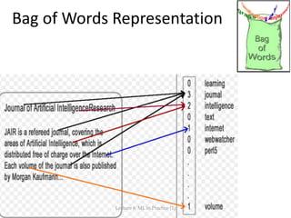
• Transform Data: FEATURE REPRESENTATION happens here.
• Model Data: Create models, evaluate them and tune them.
[...] (tasks after here…)
Lecture 8: ML in Practice (1)

11. Feature representation vs Feature
Selection
• Feature representation is different from
Attribute/Feature selection
Lecture 8: ML in Practice (1)

12. Irrelevant and Reduntant Features
• Not all features have equal importance.
• Those attributes that are irrelevant to the
problem need to be removed.
• Feature selection addresses those problems
by automatically selecting a subset that are
most useful to the problem.
Lecture 8: ML in Practice (1)

13. Learning with unbalanced data
• Imbalanced data:
– The number of positive examples is dwarfed by
the number of negative examples (or viceversa)
• Solutions:
– Assign an importance weight to the minority class
– Subsampling
– Oversampling
Lecture 8: ML in Practice (1)

14. Multiclass Classification
• OVA (one versus all)
• AVA (all versus all)
• Binary tree
Lecture 8: ML in Practice (1)

15. Theoretical Models vs Real
Machine Learning Schemes
 For an algorithm to be useful in a wide
range of real-world applications it must:
 Allow missing values
 Be robust in the presence of noise
 Be able to approximate arbitrary concept
descriptions
 etc.
Lecture 8: ML in Practice (1)

16. Evaluating what’s been learned
 How predictive is the model we learned?
 Error on the training data is not a good indicator
of performance on future data
 Otherwise 1-NN would be the optimum classifier!
 Simple solution that can be used if lots of
(labeled) data is available:
 Split data into training and test set
 However: (labeled) data is usually limited
 More sophisticated techniques need to be used
Lecture 8: ML in Practice (1)

17. Issues in evaluation
 Statistical reliability of estimated differences in
performance ( significance tests)
 Choice of performance measure:
 Number of correct classifications
 Accuracy of probability estimates
 Costs assigned to different types of errors
 Many practical applications involve costs
Lecture 8: ML in Practice (1)

18. Training and testing: empirical error
 Natural performance measure for
classification problems: error rate
 Success: instance’s class is predicted correctly
 Error: instance’s class is predicted incorrectly
 Error rate: proportion of errors made over the
whole set of instances
 Empirical (Resubstitution) error: error rate
obtained from training data
 Empirical (Resubstitution) error is
(hopelessly) optimistic!
Lecture 8: ML in Practice (1)

19. Training and testing:
development/validation set & parameter
tuning
 It is important that the test data is not used in any
way to create the classifier
 Some learning schemes operate in two stages:
 Stage 1: build the basic model
 Stage 2: optimize parameter settings
 The test data can’t be used for parameter tuning!
 Proper procedure uses three sets: training data,
validation data, and test data
 Validation data is used to optimize parameters
Lecture 8: ML in Practice (1)

20. Training and testing: test set
 Test set: independent instances that have played
no part in formation of classifier
 Assumption: both training data and test data are
representative samples of the underlying problem
 Test and training data may differ in nature
 Example: classifiers built using customer data from two
different towns A and B
 To estimate performance of classifier from town A in completely
new town, test it on data from B
Lecture 8: ML in Practice (1)

21. Making the most of the data
 Once evaluation is complete, all the data can be
used to build the final classifier
 Generally, the larger the training data the better
the classifier (but returns diminish)
 The larger the test data the more accurate the
error estimate
 Holdout procedure: method of splitting original
data into training and test set
 Dilemma: ideally both training set and test set should be
large!
Lecture 8: ML in Practice (1)

22. Holdout estimation
 What to do if the amount of data is limited?
 The holdout method reserves a certain amount
for testing and uses the remainder for training
 Usually: one third for testing, the rest for training
 Problem: the samples might not be
representative
 Example: class might be missing in the test data
 Advanced version uses stratification
 Ensures that each class is represented with
approximately equal proportions in both subsets
Lecture 8: ML in Practice (1)

23. Repeated holdout method
 Holdout estimate can be made more reliable by
repeating the process with different subsamples
 In each iteration, a certain proportion is randomly
selected for training (possibly with stratificiation)
 The error rates on the different iterations are averaged to
yield an overall error rate
 This is called the repeated holdout method
 Still not optimum: the different test sets overlap
 Can we prevent overlapping?
Lecture 8: ML in Practice (1)

24. Cross-validation
 Cross-validation avoids overlapping test sets
 First step: split data into k subsets of equal size
 Second step: use each subset in turn for testing,
the remainder for training
 Called k-fold cross-validation
 Often the subsets are stratified before the
cross-validation is performed
 The error estimates are averaged to yield an
overall error estimate
Lecture 8: ML in Practice (1)

25. More on cross-validation
 Standard method for evaluation: stratified ten-fold
cross-validation
 Why ten?
 Extensive experiments have shown that this is the best
choice to get an accurate estimate
 There is also some theoretical evidence for this
 Stratification reduces the estimate’s variance
 Even better: repeated stratified cross-validation
 E.g. ten-fold cross-validation is repeated ten times and
results are averaged (reduces the variance)
Lecture 8: ML in Practice (1)

26. Leave-One-Out cross-validation
 Leave-One-Out:
a particular form of cross-validation:
 Set number of folds to number of training instances
 I.e., for n training instances, build classifier n times
 Makes best use of the data
 Involves no random subsampling
 Very computationally expensive
 (exception: NN)
Lecture 8: ML in Practice (1)

27. Leave-One-Out-CV and stratification
 Disadvantage of Leave-One-Out-CV:
stratification is not possible
 It guarantees a non-stratified sample
because there is only one instance in the
test set!
Lecture 8: ML in Practice (1)

28. The bootstrap
 CV uses sampling without replacement
 The same instance, once selected, can not be selected
again for a particular training/test set
 The bootstrap uses sampling with
replacement to form the training set
 Sample a dataset of n instances n times with
replacement to form a new dataset of n instances
 Use this data as the training set
 Use the instances from the original
dataset that don’t occur in the new
training set for testing
Lecture 8: ML in Practice (1)

29. The 0.632 bootstrap
 Also called the 0.632 bootstrap
 A particular instance has a probability of
1–1/n of not being picked
 Thus its probability of ending up in the
test data is:
 This means the training data will contain
approximately 63.2% of the instances
Lecture 8: ML in Practice (1)

30. Estimating error with the bootstrap
 The error estimate on the test data will be
very pessimistic
 Trained on just ~63% of the instances
 Therefore, combine it with the
resubstitution/empirical error:
 The resubstitution/empirical error gets less
weight than the error on the test data
 Repeat process several times with different
replacement samples; average the results
Lecture 8: ML in Practice (1)

31. More on the bootstrap
 Probably the best way of estimating
performance for very small datasets
 However, it has some problems….
Lecture 8: ML in Practice (1)

32. The end
Lecture 8: ML in Practice (1)