Role of interpolation and sampling in image operation

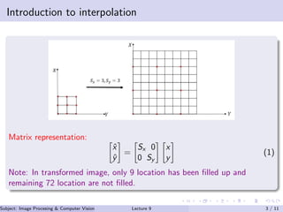
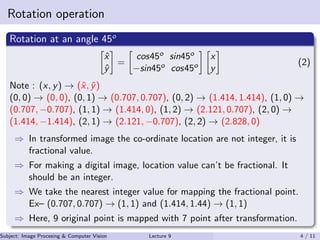
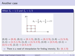
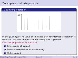
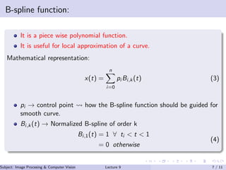
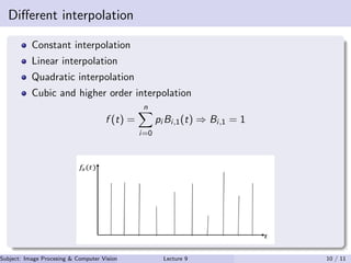
1. Role of Interpolation and Resampling in Image Operation
Subject: Image Procesing & Computer Vision
Dr. Varun Kumar
Subject: Image Procesing & Computer Vision Dr. Varun Kumar (IIIT Surat)Lecture 9 1 / 11

2. Outlines
1 Introduction to interpolation
2 Fundamental sampling operation
3 B-spline function
4 References
Subject: Image Procesing & Computer Vision Dr. Varun Kumar (IIIT Surat)Lecture 9 2 / 11

3. Introduction to interpolation
Matrix representation:
ˆx
ˆy
=
Sx 0
0 Sy
x
y
(1)
Note: In transformed image, only 9 location has been filled up and
remaining 72 location are not filled.
Subject: Image Procesing & Computer Vision Dr. Varun Kumar (IIIT Surat)Lecture 9 3 / 11

4. Rotation operation
Rotation at an angle 45o
ˆx
ˆy
=
cos45o sin45o
−sin45o cos45o
x
y
(2)
Note : (x, y) → (ˆx, ˆy)
(0, 0) → (0, 0), (0, 1) → (0.707, 0.707), (0, 2) → (1.414, 1.414), (1, 0) →
(0.707, −0.707), (1, 1) → (1.414, 0), (1, 2) → (2.121, 0.707), (2, 0) →
(1.414, −1.414), (2, 1) → (2.121, −0.707), (2, 2) → (2.828, 0)
⇒ In transformed image the co-ordinate location are not integer, it is
fractional value.
⇒ For making a digital image, location value can’t be fractional. It
should be an integer.
⇒ We take the nearest integer value for mapping the fractional point.
Ex– (0.707, 0.707) → (1, 1) and (1.414, 1.44) → (1, 1)
⇒ Here, 9 original point is mapped with 7 point after transformation.
Subject: Image Procesing & Computer Vision Dr. Varun Kumar (IIIT Surat)Lecture 9 4 / 11

5. Another case
When Sx = 1/3 and Sy = 1/3
(0, 0) → (0, 0), (0, 1) → (0, 1/3), (0, 2) → (0, 2/3), (1, 0) → (1/3, 0),
(1, 1) → (1/3, 1/3), (1, 2) → (1/3, 2/3), (2, 0) → (2/3, 0), (2, 1) →
(2/3, 1/3), (2, 2) → (2/3, 2/3)
⇒ There is a need of interpolation for finding intensity. Ex- (0, 1/3)
Subject: Image Procesing & Computer Vision Dr. Varun Kumar (IIIT Surat)Lecture 9 5 / 11

6. Resampling and interpolation
1D sampling operation
In this given figure, no value of amplitude exist for intermediate location in
time axis. We need interpolation for solving such a problem.
Desirable properties of interpolation:
1 Finite region of support
2 Smooth interpolation no-discontinuity
3 Shift invariant
Subject: Image Procesing & Computer Vision Dr. Varun Kumar (IIIT Surat)Lecture 9 6 / 11

7. B-spline function:
It is a piece wise polynomial function.
It is useful for local approximation of a curve.
Mathematical representation:
x(t) =
n
i=0
pi Bi,k(t) (3)
pi → control point how the B-spline function should be guided for
smooth curve.
Bi,k(t) → Normalized B-spline of order k
Bi,1(t) = 1 ∀ ti < t < 1
= 0 otherwise
(4)
Subject: Image Procesing & Computer Vision Dr. Varun Kumar (IIIT Surat)Lecture 9 7 / 11

8. Continued–
Bi,k(t) =
(t − ti )Bi,k−1(t)
ti+k−1 − ti
+
(ti+1 − 1)Bi+1,k1(t)
ti+k − ti+1
(5)
Conversion
Bi,k(t) = B0,k(t − i)
or
B0,1(t) = 1 ∀ 0 ≤ t < 1
= 0 otherwise
(6)
or
B0,2(t) = t ∀ 0 ≤ t < 1
= 2 − t ∀ 1 ≤ t < 2
= 0 otherwise
(7)
Subject: Image Procesing & Computer Vision Dr. Varun Kumar (IIIT Surat)Lecture 9 8 / 11

9. Continued–
B0,3(t) = t2
/2 ∀ 0 ≤ t < 1
= −t2
+ 3t − 1.5 ∀ 1 ≤ t < 2
= (3 − t)2
/2 ∀ 2 ≤ t < 3
= 0 otherwise
(8)
or
B0,4(t) = t3
/6 ∀ 0 ≤ t < 1
=
−3t3 + 12t2 − 12t + 4
6
∀ 1 ≤ t < 2
=
3t3 − 24t2 + 60t − 44
6
∀ 2 ≤ t < 3
=
(4 − t)3
6
∀ 3 ≤ t < 4
= 0 otherwise
(9)
Subject: Image Procesing & Computer Vision Dr. Varun Kumar (IIIT Surat)Lecture 9 9 / 11

10. Different interpolation
Constant interpolation
Linear interpolation
Quadratic interpolation
Cubic and higher order interpolation
f (t) =
n
i=0
pi Bi,1(t) ⇒ Bi,1 = 1
Subject: Image Procesing & Computer Vision Dr. Varun Kumar (IIIT Surat)Lecture 9 10 / 11

11. References
M. Sonka, V. Hlavac, and R. Boyle, Image processing, analysis, and machine vision.
Cengage Learning, 2014.
D. A. Forsyth and J. Ponce, “A modern approach,” Computer vision: a modern
approach, vol. 17, pp. 21–48, 2003.
L. Shapiro and G. Stockman, “Computer vision prentice hall,” Inc., New Jersey,
2001.
R. C. Gonzalez, R. E. Woods, and S. L. Eddins, Digital image processing using
MATLAB. Pearson Education India, 2004.
Subject: Image Procesing & Computer Vision Dr. Varun Kumar (IIIT Surat)Lecture 9 11 / 11