This manuscript address the linear smoothing, median, and sharpening filter operation for image processing

1. Linear Smoothing, Median, and Sharpening Filter
Subject: Image Procesing & Computer Vision
Dr. Varun Kumar
Subject: Image Procesing & Computer Vision Dr. Varun Kumar (IIIT Surat)Lecture 20 1 / 10

2. Outlines
1 Mask processing technique
Linear smoothing filter
Median filter (nonlinear filter)
Sharpening filter
2 References
Subject: Image Procesing & Computer Vision Dr. Varun Kumar (IIIT Surat)Lecture 20 2 / 10

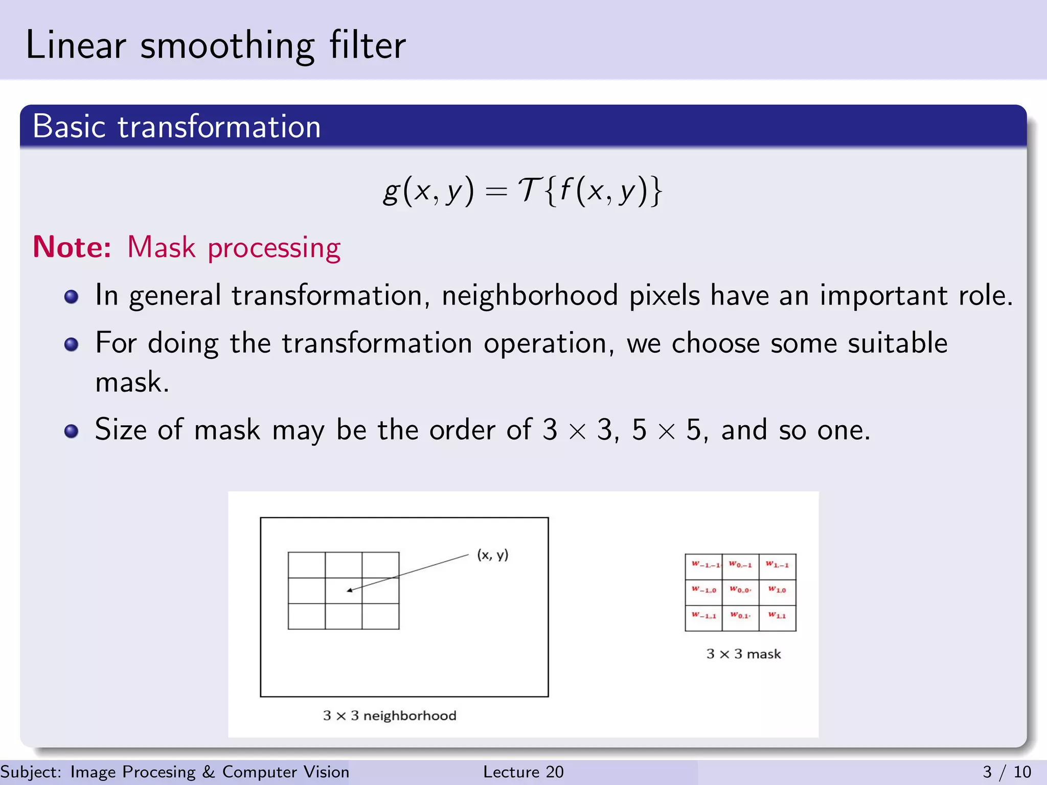
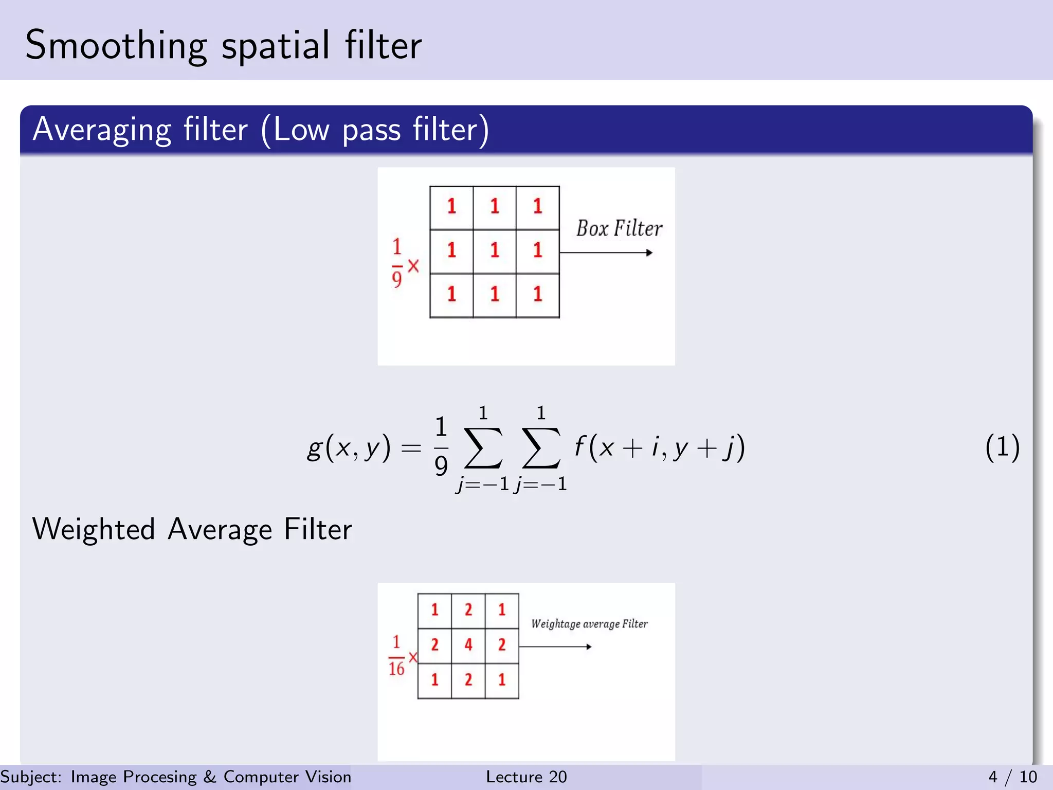
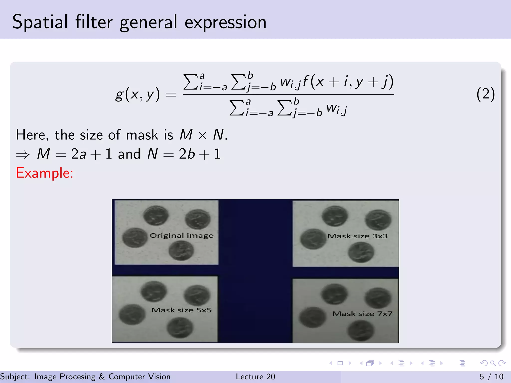
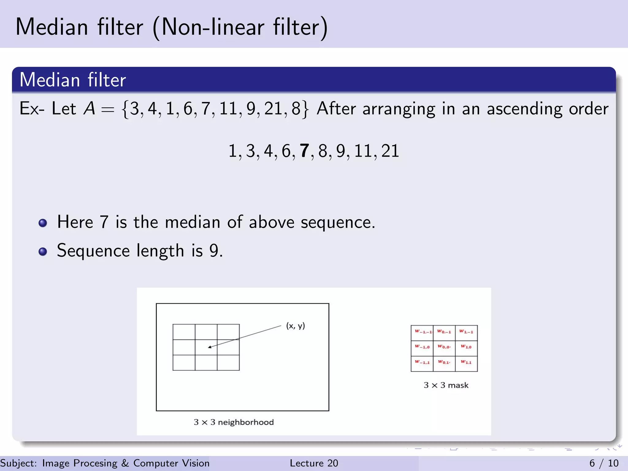
3. Linear smoothing filter
Basic transformation
g(x, y) = T {f (x, y)}
Note: Mask processing
In general transformation, neighborhood pixels have an important role.
For doing the transformation operation, we choose some suitable
mask.
Size of mask may be the order of 3 × 3, 5 × 5, and so one.
Subject: Image Procesing & Computer Vision Dr. Varun Kumar (IIIT Surat)Lecture 20 3 / 10

4. Smoothing spatial filter
Averaging filter (Low pass filter)
g(x, y) =
1
9
1
j=−1
1
j=−1
f (x + i, y + j) (1)
Weighted Average Filter
Subject: Image Procesing & Computer Vision Dr. Varun Kumar (IIIT Surat)Lecture 20 4 / 10

5. Spatial filter general expression
g(x, y) =
a
i=−a
b
j=−b wi,j f (x + i, y + j)
a
i=−a
b
j=−b wi,j
(2)
Here, the size of mask is M × N.
⇒ M = 2a + 1 and N = 2b + 1
Example:
Subject: Image Procesing & Computer Vision Dr. Varun Kumar (IIIT Surat)Lecture 20 5 / 10

6. Median filter (Non-linear filter)
Median filter
Ex- Let A = {3, 4, 1, 6, 7, 11, 9, 21, 8} After arranging in an ascending order
1, 3, 4, 6, 7, 8, 9, 11, 21
Here 7 is the median of above sequence.
Sequence length is 9.
Subject: Image Procesing & Computer Vision Dr. Varun Kumar (IIIT Surat)Lecture 20 6 / 10

7. Sharpening spatial filter
First order derivative filter
Must be zeros in areas of constant gray scale value.
Non-zero at the on set of the gray level step or ramp.
Non-zero along ramp
Second order derivative filter
Zeros in flat areas.
Non-zero at the on set of the gray level step or ramp.
Zero along ramps of constant slope.
df (x)
dx
= lim
∆x→0
f (x + ∆x) − f (x)
∆x
∂f (x)
∂x
= f (x + 1) − f (x)
Subject: Image Procesing & Computer Vision Dr. Varun Kumar (IIIT Surat)Lecture 20 7 / 10

8. Second order derivative
If f (x) is continuous domain expression then d2f (x)
dx2 is called as the 2nd
order derivative. In discrete domain
∂2f (x)
∂x2
= f (x + 1) + f (x − 1) − 2f (x)
Laplacian operator
∆2
f =
∂2f
∂x2
+
∂2f
∂y2
For 2D signal
∂2f
∂x2
= f (x + 1, y) + f (x − 1, y) − 2f (x, y)
∂2f
∂y2
= f (x, y + 1) + f (x, y − 1) − 2f (x, y)
Subject: Image Procesing & Computer Vision Dr. Varun Kumar (IIIT Surat)Lecture 20 8 / 10

9. Laplacian operator
∆2
f = f (x + 1, y) + f (x − 1, y) + f (x, y + 1) + f (x, y − 1) − 4f (x, y)
Laplacian mask
Subject: Image Procesing & Computer Vision Dr. Varun Kumar (IIIT Surat)Lecture 20 9 / 10

10. References
M. Sonka, V. Hlavac, and R. Boyle, Image processing, analysis, and machine vision.
Cengage Learning, 2014.
D. A. Forsyth and J. Ponce, “A modern approach,” Computer vision: a modern
approach, vol. 17, pp. 21–48, 2003.
L. Shapiro and G. Stockman, “Computer vision prentice hall,” Inc., New Jersey,
2001.
R. C. Gonzalez, R. E. Woods, and S. L. Eddins, Digital image processing using
MATLAB. Pearson Education India, 2004.
Subject: Image Procesing & Computer Vision Dr. Varun Kumar (IIIT Surat)Lecture 20 10 / 10