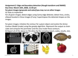
Download as PDF, PPTX
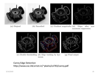
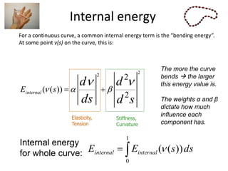
![3/19/2020 3
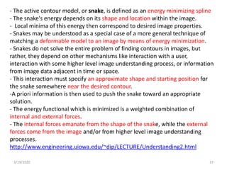
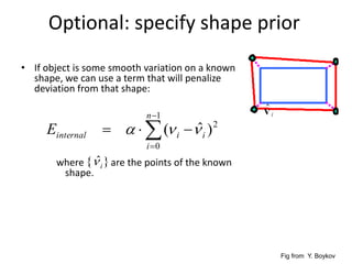
Edge Detection Goal: Could you point out the most “salient” or “strongest” edges or
the object boundaries? [Szeliski's Book p.210]](https://image.slidesharecdn.com/lecture-45-sbe404edgedetectioncodechainshoughtransformsnakes-200821100417/85/Lecture-4-5-computer-vision-edge-detection-code-chains-hough-transform-snakes-3-320.jpg)
![3/19/2020 5
[Ch. 14, Practical Image and Video Processing Using MATLAB by Oge Marques]](https://image.slidesharecdn.com/lecture-45-sbe404edgedetectioncodechainshoughtransformsnakes-200821100417/85/Lecture-4-5-computer-vision-edge-detection-code-chains-hough-transform-snakes-5-320.jpg)
![3/19/2020 7
[Ch. 14,
Practical
Image
and Video
Processin
g Using
MATLAB
by Oge
Marques]
Even low noise levels can corrupt the edge detection operation…](https://image.slidesharecdn.com/lecture-45-sbe404edgedetectioncodechainshoughtransformsnakes-200821100417/85/Lecture-4-5-computer-vision-edge-detection-code-chains-hough-transform-snakes-7-320.jpg)
![3/19/2020 10
[Ch. 14,
Practical
Image and
Video
Processing
Using
MATLAB by
Oge
Marques]](https://image.slidesharecdn.com/lecture-45-sbe404edgedetectioncodechainshoughtransformsnakes-200821100417/85/Lecture-4-5-computer-vision-edge-detection-code-chains-hough-transform-snakes-10-320.jpg)
![3/19/2020 11
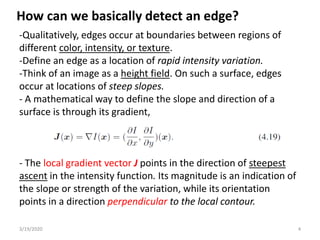
- Estimate the gray-level gradient at a pixel, which can be approximated by the
digital equivalent of the first-order derivative as follows [Marques’ book, p.338]:
- The gradients are often computed within a 3×3 neighborhood using convolution:
where the Prewitt kernels are given by:
Example 1: Prewitt Edge Detector (First-order
Detector)](https://image.slidesharecdn.com/lecture-45-sbe404edgedetectioncodechainshoughtransformsnakes-200821100417/85/Lecture-4-5-computer-vision-edge-detection-code-chains-hough-transform-snakes-11-320.jpg)
![3/19/2020 12
[Ch. 14,
Practical
Image
and
Video
Processi
ng Using
MATLAB
by Oge
Marque
s]](https://image.slidesharecdn.com/lecture-45-sbe404edgedetectioncodechainshoughtransformsnakes-200821100417/85/Lecture-4-5-computer-vision-edge-detection-code-chains-hough-transform-snakes-12-320.jpg)
![3/19/2020 13
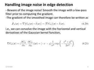
- The Laplacian operator is a straightforward digital
approximation of the second-order derivative of the intensity.
Although it has the potential for being employed as an isotropic
(i.e., omnidirectional) edge detector, it is rarely used in isolation
because of two limitations [Marques’ book, p. 343]:
• It generates “double edges,” that is, positive and negative
values for each edge.
• It is extremely sensitive to noise.
Example 2: Zero-crossing Edge Detector
(Second-order detector)](https://image.slidesharecdn.com/lecture-45-sbe404edgedetectioncodechainshoughtransformsnakes-200821100417/85/Lecture-4-5-computer-vision-edge-detection-code-chains-hough-transform-snakes-13-320.jpg)
![3/19/2020 14
[Ch. 14,
Practical
Image
and
Video
Processi
ng Using
MATLAB
by Oge
Marque
s]](https://image.slidesharecdn.com/lecture-45-sbe404edgedetectioncodechainshoughtransformsnakes-200821100417/85/Lecture-4-5-computer-vision-edge-detection-code-chains-hough-transform-snakes-14-320.jpg)
![3/19/2020 16
[Ch. 14,
Practical
Image
and
Video
Processi
ng Using
MATLAB
by Oge
Marque
s]](https://image.slidesharecdn.com/lecture-45-sbe404edgedetectioncodechainshoughtransformsnakes-200821100417/85/Lecture-4-5-computer-vision-edge-detection-code-chains-hough-transform-snakes-16-320.jpg)
![3/19/2020 17
[Ch. 14,
Practical
Image
and
Video
Processi
ng Using
MATLAB
by Oge
Marque
s]](https://image.slidesharecdn.com/lecture-45-sbe404edgedetectioncodechainshoughtransformsnakes-200821100417/85/Lecture-4-5-computer-vision-edge-detection-code-chains-hough-transform-snakes-17-320.jpg)
![3/19/2020 20
[Ch. 14,
Practical
Image
and
Video
Processi
ng Using
MATLAB
by Oge
Marque
s]](https://image.slidesharecdn.com/lecture-45-sbe404edgedetectioncodechainshoughtransformsnakes-200821100417/85/Lecture-4-5-computer-vision-edge-detection-code-chains-hough-transform-snakes-20-320.jpg)
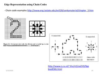
![3/19/2020 23
Edge Representation using Chain Codes [Szeliski's Book p.217]
- Linked edgel lists can be encoded more compactly using a variety of alternative
representations.
A chain code encodes a list of connected points lying on an N-8 grid using a
three-bit code corresponding to the eight cardinal directions (N, NE, E, SE, S, SW, W, NW)
between a point and its successor (Figure 4.34).
-While this representation is more compact than the original edgel list (especially if
predictive variable-length coding is used), it is not very suitable for further processing.
-See: Introduction to Chain Codes
http://www.mind.ilstu.edu/curriculum/chain_codes_intro/chain_codes_intro.php](https://image.slidesharecdn.com/lecture-45-sbe404edgedetectioncodechainshoughtransformsnakes-200821100417/85/Lecture-4-5-computer-vision-edge-detection-code-chains-hough-transform-snakes-23-320.jpg)
![3/19/2020 25
Edge Representation using Arc-Length Parameterization [Szeliski's Book p.217]
- A more useful representation is the arc length parameterization of a contour, x(s), where
s denotes the arc length along a curve (Figure 4.35).](https://image.slidesharecdn.com/lecture-45-sbe404edgedetectioncodechainshoughtransformsnakes-200821100417/85/Lecture-4-5-computer-vision-edge-detection-code-chains-hough-transform-snakes-25-320.jpg)
![3/19/2020 26
Edge Representation using Arc-Length Parameterization [Szeliski's Book p.217]
- The advantage of the arc-length parameterization is that it makes matching and
processing (e.g., smoothing) operations much easier (Figure 4.36). Arc-length
parameterization can also be used to smooth curves in order to remove digitization noise.](https://image.slidesharecdn.com/lecture-45-sbe404edgedetectioncodechainshoughtransformsnakes-200821100417/85/Lecture-4-5-computer-vision-edge-detection-code-chains-hough-transform-snakes-26-320.jpg)
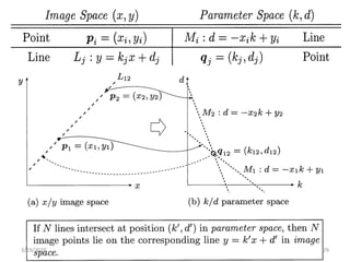
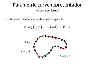
![3/19/2020 28
Points and lines
in image and
parameter spaces
http://books.google.com.eg/books/abou
t/Digital_Image_Processing.html?id=jCEi
9MVfxD8C&redir_esc=y
[Chapter 9]](https://image.slidesharecdn.com/lecture-45-sbe404edgedetectioncodechainshoughtransformsnakes-200821100417/85/Lecture-4-5-computer-vision-edge-detection-code-chains-hough-transform-snakes-28-320.jpg)
![3/19/2020 30
Line Detection using Hough Tranform [Szeliski's Book p.221]
Motivation: Lines in the real world are sometimes broken up into disconnected
components or made up of many collinear line segments. In many cases, it is desirable to
group such collinear segments into extended lines.
Original Formulation: Each edge point votes for all possible lines passing through it, and
lines corresponding to high accumulator or bin values are examined for potential line fits.](https://image.slidesharecdn.com/lecture-45-sbe404edgedetectioncodechainshoughtransformsnakes-200821100417/85/Lecture-4-5-computer-vision-edge-detection-code-chains-hough-transform-snakes-30-320.jpg)
![3/19/2020 31
Line Detection using Hough Tranform [Szeliski's Book p.222]
Alternate Formulation: Use the local orientation information at each edgel
to vote for a single accumulator cell.](https://image.slidesharecdn.com/lecture-45-sbe404edgedetectioncodechainshoughtransformsnakes-200821100417/85/Lecture-4-5-computer-vision-edge-detection-code-chains-hough-transform-snakes-31-320.jpg)
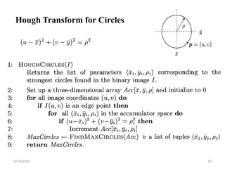
![3/19/2020 32
Line Detection using Hough Tranform [Szeliski's Book p.223]](https://image.slidesharecdn.com/lecture-45-sbe404edgedetectioncodechainshoughtransformsnakes-200821100417/85/Lecture-4-5-computer-vision-edge-detection-code-chains-hough-transform-snakes-32-320.jpg)
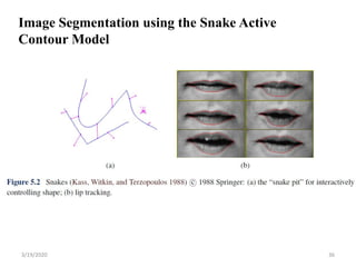
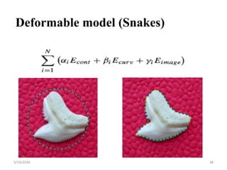
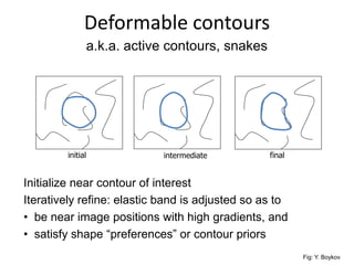
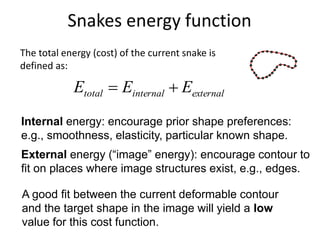
![Deformable contours
Given: initial contour (model) near desired object
a.k.a. active contours, snakes
(Single frame)
Fig: Y. Boykov
[Snakes: Active contour models, Kass, Witkin, & Terzopoulos, ICCV1987]](https://image.slidesharecdn.com/lecture-45-sbe404edgedetectioncodechainshoughtransformsnakes-200821100417/85/Lecture-4-5-computer-vision-edge-detection-code-chains-hough-transform-snakes-39-320.jpg)
![Deformable contours
Given: initial contour (model) near desired object
a.k.a. active contours, snakes
(Single frame)
Fig: Y. Boykov
Goal: evolve the contour to fit exact object boundary
[Snakes: Active contour models, Kass, Witkin, & Terzopoulos, ICCV1987]](https://image.slidesharecdn.com/lecture-45-sbe404edgedetectioncodechainshoughtransformsnakes-200821100417/85/Lecture-4-5-computer-vision-edge-detection-code-chains-hough-transform-snakes-40-320.jpg)
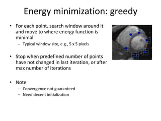
![Dealing with missing data
• The smoothness constraint can deal with missing data:
[Figure from Kass et al. 1987]](https://image.slidesharecdn.com/lecture-45-sbe404edgedetectioncodechainshoughtransformsnakes-200821100417/85/Lecture-4-5-computer-vision-edge-detection-code-chains-hough-transform-snakes-55-320.jpg)
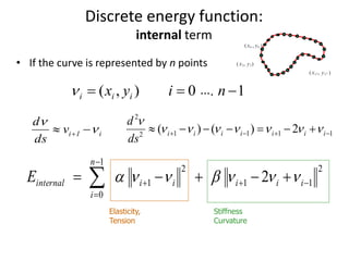

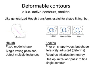
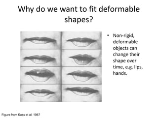
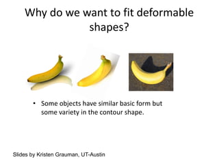
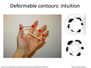
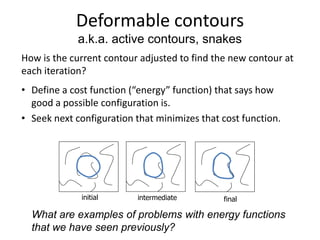
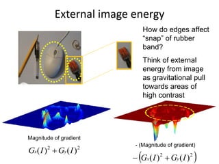
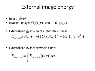
The document provides an overview of computer vision techniques including edge detection, edge representation using chain codes, line and circle detection using Hough transforms, and active contour deformable models (snakes). It describes several common edge detection algorithms like Prewitt, Laplacian of Gaussian (LoG), and Canny edge detectors. It also explains how the Hough transform can be used to detect lines and circles and discusses snakes, where an active contour model is defined as an energy minimizing spline that deforms to fit desired image properties by minimizing internal and external energy terms.