Download as PDF, PPTX

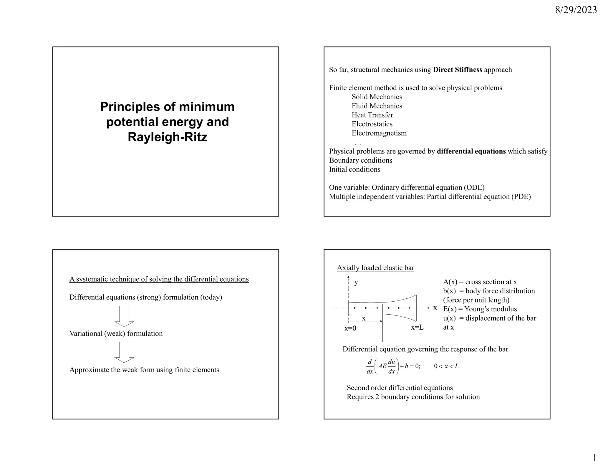
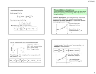
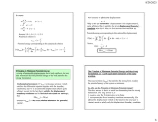
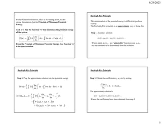
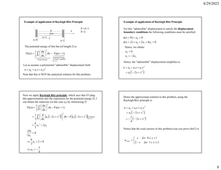

1) The document discusses principles of minimum potential energy and the Rayleigh-Ritz method for solving differential equations that arise from physical problems using finite elements. 2) It introduces the concept of minimizing the total potential energy of a system according to the principle of minimum potential energy. 3) The Rayleigh-Ritz method approximates the solution by assuming the solution is a linear combination of known functions and determining the coefficients by minimizing the potential energy.


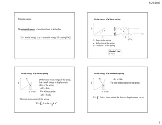
![[Deck] What's New in Spark-Iceberg Integration via DSV2.pptx](https://cdn.slidesharecdn.com/ss_thumbnails/deckwhatsnewinspark-icebergintegrationviadsv2-260210005337-25955b12-thumbnail.jpg?width=640&height=640&fit=bounds)

