REPORT SUMMARY Vibration refers to a mechanical phenomenon involving oscillations about a point. These oscillations can be of any imaginable range of amplitudes and frequencies, with each combination having its own effect. These effects can be positive and purposefully induced, but they can also be unintentional and catastrophic. It's therefore imperative to understand how to classify and model vibration. Within the classroom portion of ME 345, we discussed damped and undamped vibrations, appropriate models, and several of their properties. The purpose of Lab 3 is to give us the corresponding "hands-on" experience to cement our understanding of the theory. As it turns out, vibration can be modeled with a simple spring-mass system (spring-mass-damper system for damped vibration). In order to create a mathematical model for our simple spring-mass system, we apply Newton's second law and sum the forces about the mass. After applying some of our knowledge of differential equations, the result is a second order linear differential equation (in vector form). This can easily be converted to the scalar version, from which it's easy to glean various properties of the vibration (i.e. natural frequency, period, etc.). In the lab, we were provided with a PASCO motion sensor, USB link, ramp, and accompanying software. All of the aforementioned equipment was already assembled and connected. The ramp was set up at an angle with a stop on the elevated end and the motion sensor on the lower end. The sensor was connected to the USB link, which was in turn connected to the computer. We chose to use the Xplorer GLX software to interface with the sensor and record our data. After receiving our equipment, we gathered data on our spring's extension with a known load to derive a spring constant. We were provided with a small cart to which we attached weights to increase its mass. In order to model free vibration, we placed the cart on the track and attached it to the stop at the top of the ramp with a spring. After displacing the cart a certain distance from its equilibrium point, the cart was released and was allowed to oscillate on the track while we recorded its distance from the sensor. This was done with displacements of -20cm, -10cm, +10cm, and +20cm from the system's equilibrium point. After gathering this data for the "free" case, a magnet was attached to the front of the car, spaced as far from the track as possible. As the track is magnetic, this caused a slight damping effect, basically converting our spring-mass system to an underdamped spring-mass-damper system. After repeating the procedure for the "free" case, we moved the magnets as close to the track as possible (causing the system to become overdamped) and again repeated the procedure for the "free" case. We were finally able to determine the period, phase angle, damping coefficients, and circular and cyclical frequencies for the three systems. There were similarities and differ ...

1. REPORT SUMMARY
Vibration refers to a mechanical phenomenon involving
oscillations about a point. These oscillations can be of any
imaginable range of amplitudes and frequencies, with each
combination having its own effect. These effects can be
positive and purposefully induced, but they can also be
unintentional and catastrophic. It's therefore imperative to
understand how to classify and model vibration.
Within the classroom portion of ME 345, we discussed damped
and undamped vibrations, appropriate models, and several of
their properties. The purpose of Lab 3 is to give us the
corresponding "hands-on" experience to cement our
understanding of the theory.
As it turns out, vibration can be modeled with a simple spring-
mass system (spring-mass-damper system for damped
vibration). In order to create a mathematical model for our
simple spring-mass system, we apply Newton's second law and
sum the forces about the mass. After applying some of our
knowledge of differential equations, the result is a second order
linear differential equation (in vector form). This can easily be
converted to the scalar version, from which it's easy to glean
various properties of the vibration (i.e. natural frequency,
period, etc.).
In the lab, we were provided with a PASCO motion sensor, USB
link, ramp, and accompanying software. All of the

2. aforementioned equipment was already assembled and
connected. The ramp was set up at an angle with a stop on the
elevated end and the motion sensor on the lower end. The
sensor was connected to the USB link, which was in turn
connected to the computer. We chose to use the Xplorer GLX
software to interface with the sensor and record our data. After
receiving our equipment, we gathered data on our spring's
extension with a known load to derive a spring constant. We
were provided with a small cart to which we attached weights to
increase its mass. In order to model free vibration, we placed
the cart on the track and attached it to the stop at the top of the
ramp with a spring. After displacing the cart a certain distance
from its equilibrium point, the cart was released and was
allowed to oscillate on the track while we recorded its distance
from the sensor. This was done with displacements of -20cm, -
10cm, +10cm, and +20cm from the system's equilibrium point.
After gathering this data for the "free" case, a magnet was
attached to the front of the car, spaced as far from the track as
possible. As the track is magnetic, this caused a slight damping
effect, basically converting our spring-mass system to an
underdamped spring-mass-damper system. After repeating the
procedure for the "free" case, we moved the magnets as close to
the track as possible (causing the system to become
overdamped) and again repeated the procedure for the "free"
case.
We were finally able to determine the period, phase angle,
damping coefficients, and circular and cyclical frequencies for
the three systems. There were similarities and differences in
the results, including the finding that the period for all of the
systems across all of the displacements are nearly identical (in
some cases, up to two decimal places). A potential trend
observed was the increase of damping as the magnetic damper
increased its proximity to the track. For derivations, data
visualization, and further results, please see the Results and
Discussion section.
In this lab we took our theoretical vibration knowledge and

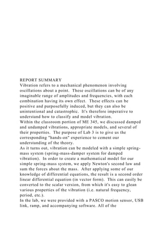
3. applied it to data gathered in the real world. As our
measurements and calculations show, the theoretical values of
many components of vibrating systems very closely match their
empirically measured corollaries. For detailed results,
derivations, etc., please see the Results and Discussion section.
results and discussion
The following figures display a summary of our results. For
further detail and the raw data, please see the Appendix.
Figure 1: Plot of all free vibration data
Figure 2: Plot of all underdamped vibration data
Figure 3: Plot of all overdamped data
In the experiment, we gathered three sets of displacement vs.
time data. The first was from the "free" vibration system
(plotted in Figure 1), the second was from the "underdamped"
system (plotted in Figure 2), and the third was from the
"overdamped" system (plotted in Figure 3). The "free" system
clearing shows damping, but definitely oscillated for a greater
amount of time than the "underdamped" or "overdamped"
systems, which is at least partially in line with expectations.
The "underdamped" and "overdamped" systems acted as
expected, with "underdamped" oscillating much longer than
"overdamped", which only oscillated for about 1.5 periods.
The first section of the results and discussion portion of the lab
required a derivation of the scalar equation of motion of the
"free" system. This was essentially a spring-mass system on an
inclined plane of approximately 10 degrees. For a detailed
derivation, see the work in the appendix, a brief overview
follows. After creating the free body diagram of this system,

4. Newton's second law was applied (see Equation 1).
Equation 1: Newton's second law
It is known from the free body diagram that the total force on
the mass was the sum of the spring force and the gravity
component along the mass' axis of motion. Substituting the
spring force's constituents into the equation (spring
displacement and spring constant) and then converting the
resulting linear ordinary differential equation (ODE) into a
scalar resulted in Equation 2.
Equation 2: "Free" system scalar equation
Then, in reference to the "free" system, the period (Τ), circular
natural frequency (ωn), cyclical natural frequency (f), and phase
angle (ɸ) were required. These quantities were determined from
the graph. The period was found by taking the time difference
of two sequential "peaks" of each curve, resulting in Τ-20 = 3
seconds, Τ-10 = 3 seconds, Τ+10 = 3.2 seconds, and Τ+20 = 3
seconds.
Equation 3: Natural circular frequency/period relation
Now that we had the period for each of the curves, we used
Equation 3 to determine each of their natural frequencies: ωn -
20 =2.09 rad/s, ωn -10 =2.09 rad/s, ωn +10 =1.96 rad/s, and ωn
+20 =2.09 rad/s.
Equation 4: Cyclical frequency/period relation
Figure 4: Phase angle definition from class notes
Equation 5: Phase angle equation
With the relation described in Equation 4, we were able to
determine the following natural cyclical frequencies: f-20 =
0.33 hz, f-10 = 0.33 hz, f+10 = 0.3125 hz, f+20 = 0.33 hz.
From the description of the phase angle in class (Figure 4), we

5. determined that the difference referred to between the two
curves would always be consistent with the definition at y(0).
This allowed us to construct Equation 5 and generate the
following results: ɸ-20 = 1.78 (lag), ɸ-10 = 1.25 (lag), ɸ+10 =
1.176 (lead), and ɸ+20 = 1.78 (lead).
Equation 6: Theoretical natural frequency
Next, the lab required a comparison of the theoretical and
experimentally measured natural frequency. As the theoretical
only depends on the spring constant (previously determined
experimentally with the spring force relation) and the mass of
the mass in the system, it will be a constant ωn = 2.09 for all
initial displacements. Impressively, this identically matches 3
or 4 experimentally measured results (to two decimal places),
with the third likely anomalous, but still very close. This is a
good indicator that the theoretical equation very closely (again,
in this case, identically) models the actual natural circular
frequency. From the data gathered, it's clear that the circular
natural frequency and period do not depend on the initial
displacement (given all 4 values in these two cases are nearly
identical). However, it's also clear that the phase angle data is
significantly different, divided into two groups based on the
magnitude of the initial displacement, therefore the phase angle
is clearly affected by the initial displacement. Sadly, the graph
of the "free" system shows that each curve has a decreasing
amplitude as time increases. While it's disappointing that our
"free" system is therefore clearly not perfectly free, it's perhaps
worse that the lab then requires more work. To determine the
damping coefficient (c), the logarithmic decrement method was
used, as described in Equation 7, to determine c-20 = 0.01, c-20
= 0.009, c+10 = 0.008, c+20 = 0.01. All the values for the
damping coefficient are approximately 0.01, showing that there
is essentially no dependence on initial displacement (and
therefore no variation in c due to variation in the initial
displacement of the spring).

6. Equation 7: Damping coefficient
For the second portion of the results and discussion, the
underdamped and overdamped data was analyzed. First,
Newton's second law was again used to derive the scalar
equation of motion. This was identical to the free system with
the addition of a damping force.
Equation 8: Scalar equation of motion for damped system
Specifically requested were the period (Τd), circular natural
frequency (ωd), cyclical natural frequency (f), and phase angle
(ɸ) were required. These quantities were determined from the
graph. The period was found by taking the time difference of
two sequential "peaks" of each curve, resulting in Τd-20 =
3.3030 seconds, Τd-10 = 3.3030 seconds, Τd+10 =
3.0031seconds, and Τd+20 = 3.3031 seconds for the
overdamped system and Τd-20 = 3.1999 seconds, Τd-10 =
3.0999 seconds, Τd+10 = 2.8999seconds, and Τd+20 = 3.0999
seconds for the underdamped system.
With the period for each of the curves, applying Equation 8
yielded the damped circular natural frequencies; ωd -20 =1.9022
rad/s, ωd -10 =2.092302 rad/s, ωd +10 =2.0922 rad/s, and ωd
+20 =1.9023 rad/s for overdamped and ωd -20 =1.9636 rad/s,
ωd -10 =2.0269 rad/s, ωd +10 =2.1667 rad/s, and ωd +20
=2.0269 rad/s for underdamped.
Equation 9: Damped circular natural frequency/period relation
With the relation described in Equation 9, it was possible to
determine the following damped natural cyclical frequencies: f-
20 = 0.5257 hz, f-10 = 0.47795 hz, f+10 = 0.47799 hz, f+20 =
0.526 hz for the overdamped system and f-20 = 0.3125 hz, f-10
= 0.3226 hz, f+10 = 0.3448 hz, f+20 = 0.3226 hz for the
underdamped system.
Equation 10: Damped cyclical natural frequency/period relation
From the description of the phase angle in class (Figure 4), it

7. was determined that the difference referred to between the two
curves would always be consistent with the definition at y(0).
This leads to Equation 5 and generates the following results: ɸ-
20 = 0.201021(lag), ɸ-10 = 0.1809612 (lag), ɸ+10 = 0.21102
(lead), and ɸ+20 = 0.201002 (lead) for the overdamped system
and ɸ-20 = 0.1709(lag), ɸ-10 = 0.1609 (lag), ɸ+10 = 0.2010
(lead), and ɸ+20 = 0.1609 (lead) for the underdamped system.
Equation 11: Damping ratio
Equation 10: damping ratio
Given Equation 10 (where xo and x1 are adjacent amplitudes),
the damping ratios are -10 = 0.016465,-20 = 0.0295,10 =
0.01368,20 = 1.9029 for the overdamped system and -10 =
0.1686,-20 = 0.1779,10 = 0.1656,20 = 0.1858 for the
underdamped system.
Equation 12: theoretical critical damping coefficient equation
To find the damping ratios using the decaying curve method, it
was necessary to plot the magnitudes of several consecutive
amplitudes. The overdamped graphs were far too short and
inconsistent to use this decay method, but the underdamped
curves supplied ample data. Fitting an exponential line to the
curve we were able to obtain an equation for the exponential
decay of our points, as shown in Figure 5.
Figure 5: Underdamped decay method
Using the equation shown in Figure 5, it was possible to use the
obvious boundary condition and find that the constant, c =

8. 1.1336. Equation 13 yielded β as β-10 = .0462, β-20 = .0297
β+10 = .0568 β+20 = .0338 for the underdamped system. These
damping ratios are significantly different from those derived
with the logarithmic method. For detailed work, see the
Appendix.
Equation 13: Decaying curve
The theoretical damping coefficient equation was used as a
comparison, yielding c-10 = 0.05518, c-20 = 0.98869 , c10 =
0.04585 , c20 =0.826815 for the overdamped system and c-10 =
0.565 , c-20 = 0.596 , c10 = 0.555 , c20 =0.623 for the
underdamped system. For detailed work, see the Appendix. It's
very likely that the damping coefficient is due to more than the
magnet alone, evidenced by the damping observed in the "free"
system, which occurred before the use of the magnetic damper.
The damping should increase as the distance between the
magnet and the track decreases. This wasn't found to be true at
all times in the data, but this is likely an error in the
calculations. The period is nearly the same across
displacements and damping.
It's clear that extraneous variables are present, including the
friction of the track. As shown by the damped behavior of the
"free" system, there is an unknown (or unaccounted for) force
acting on the system. It's difficult to identify these forces, but
they may or may not include friction with the track, friction
between the wheels and axels, damping forces due to shifting of
cart internal components, and aerodynamic drag.
conclusions
In conclusion, we took our theoretical knowledge out of the
classroom and gained valuable, practical, hands-on experience
applying it to real, tangible systems. Even though theoretical
models were incomplete, most of the time it was found that they
were able to describe the real world behavior with nearly zero
error. It was also discovered that some components of vibration
are the same for a system, regardless of its damping or initial

9. spring displacement (however, several vibration components are
indeed effected by these factors).
Weaknesses in the experiment were minimal, as suggested by
the strong, expected correlation visible in the results. The free
body diagram for the systems were overly simplified and clearly
didn't account for all forces involved (again, citing the very
visible problem with the "free" state -- it damps out). It was
also not possible to calibrate the equipment (range finder),
although that may introduce negligible error as we were
primarily concerned with distance displacement which should
be independent of a simple sensor bias.
Appendix
Choo, Vincent (2013) Class Notes: Vibration notes cleaned up.
ME 345 Class Notes Fall 2013. Las Cruces: New Mexico State
University.
Underdamped system work

10. Overdamped
over -10 0.0028 0.1028 0.2028 0.3028 0.4029
0.5029 0.6029 0.703 0.803 0.903
1.003099999999999 1.1031 1.203099999999999
1.303099999999999 1.403099999999999
1.503099999999999 1.6031 1.703099999999999
1.803099999999999 1.9031 2.0031
2.103100000000002 2.203100000000002 2.3031 2.4031
2.5031 2.603100000000002 2.703100000000002
2.802999999999998 2.903 3.003 3.103 3.203
3.302999999999998 3.403 3.503 3.603 3.703
3.802999999999998 3.903 4.003
4.102999999999996 4.203 4.302999999999996 4.403
4.503 4.602999999999996 4.703
4.802999999999996 4.903 5.003
5.102999999999996 5.203 5.302999999999996 5.403
5.503 5.602999999999996 5.703
5.802999999999996 5.903 6.003
6.102999999999996 6.203 6.302999999999996 6.403
6.503 6.602999999999996 6.703
6.802999999999996 6.903 7.003
7.102999999999996 7.203 7.302999999999996 7.403
7.503 7.602999999999996 7.703
7.802999999999996 7.903 8.003
8.103000000000001 8.203000000000001 8.303 8.403
8.503 8.603000000000001 8.703000000000001 8.803
8.903 9.003 9.103000000000001
9.203000000000001 9.303 9.403 9.503
9.603000000000001 9.703000000000001 9.803 0.954
0.956 0.962 0.97 0.981 0.993 1.006
1.018999999999999 1.032 1.044
1.054999999999999 1.064 1.072 1.077 1.081
1.083 1.083 1.082 1.079 1.077 1.074
1.07 1.066 1.062999999999999 1.058999999999999
1.056 1.052 1.05 1.048 1.046999999999999

11. 1.046 1.046 1.046 1.046 1.046 1.046
1.046 1.046 1.046 1.046 1.046 1.046
1.046 1.046 1.046 1.046 1.046 1.046
1.046 1.046 1.046 1.046 1.046 1.046
1.046 1.046 1.046 1.046 1.046 1.046
1.046 1.046999999999999 1.046999999999999
1.046999999999999 1.046999999999999 1.048 1.048
1.048 1.048 1.048 1.048 1.048 1.048
1.048 1.048 1.048 1.048 1.048 1.048
1.048 1.048 1.048 1.048 1.048 1.048
1.048 1.048 1.048 1.048 1.048 1.048
1.048 1.048 1.048 1.048 1.048 1.048
1.048 1.048 over -20 0.0025 0.1025 0.2025
0.3026 0.4026 0.5027 0.6028 0.7028 0.8029
0.903 1.003099999999999 1.1031
1.203199999999999 1.303199999999999
1.403299999999999 1.50329999999 9999
1.603299999999999 1.703299999999999
1.803299999999999 1.9032 2.0032 2.1032
2.203200000000001 2.3031 2.4031 2.5031
2.603100000000002 2.703 2.802999999999998 2.903
3.003 3.103 3.203 3.302999999999998 3.403
3.503 3.603 3.703 3.802999999999998 3.903
4.003 4.102999999999996 4.203
4.302999999999996 4.403 4.503
4.602999999999996 4.703 4.802999999999996 4.903
5.003 5.102999999999996 5.203
5.302999999999996 5.403 5.503
5.602999999999996 5.703 5.802999999999996 5.903
6.003 6.102999999999996 6.203 6.3029999999999
96 6.403 6.503 6.602999999999996 6.703
6.802999999999996 6.903 7.003
7.102999999999996 7.203 7.302999999999996 7.403
7.503 0.854 0.857 0.866 0.882 0.902
0.925 0.952 0.979 1.006 1.032 1.056
1.077 1.095 1.109 1.119 1.125 1.127

12. 1.125 1.121 1.115 1.107 1.098 1.088
1.078 1.068 1.058999999999999 1.05
1.042999999999999 1.036999999999999
1.032999999999999 1.028999999999999 1.028 1.028
1.028 1.03 1.030999999999999 1.032999999999999
1.034999999999999 1.038 1.04 1.042 1.044
1.046 1.048 1.048999999999999
1.048999999999999 1.048999999999999
1.048999999999999 1.048999999999999
1.048999999999999 1.048999999999999
1.048999999999999 1.048999999999999
1.048999999999999 1.048999999999999
1.048999999999999 1.048999999999999
1.048999999999999 1.048999999999999
1.048999999999999 1.048999999999999
1.048999999999999 1.048999999999999
1.048999999999999 1.048999999999999
1.048999999999999 1.048999999999999
1.048999999999999 1.048999999999999
1.048999999999999 1.048999999999999
1.048999999999999 1.048999999999999
1.048999999999999 1.048999999999999
1.048999999999999 over +10 0.0034 0.1033 0.2033
0.3033 0.4033 0.5032 0.6032 0.7032 0.8031
0.9031 1.003099999999999 1.103
1.202999999999999 1.302999999999999
1.402999999999999 1.502999999999999 1.603
1.702999999999999 1.802999999999999 1.903 2.003
2.103 2.203 2.302999999999998 2.403 2.503
2.603100000000002 2.703100000000002 2.8031 2.9031
3.0031 3.103100000000002 3.203100000000002 3.3031
3.4031 3.5031 3.603100000000002
3.703100000000002 3.8031 3.9031 4.0031 4.1031
4.2031 4.3031 4.4031 4.5031
4.603099999999999 4.7031 4.8031 4.9031 5.0031
5.1031 5.2031 5.3031 5.4031 5.5031

13. 5.603099999999999 5.7031 5.8031 5.9031 6.0031
6.1031 6.2031 6.3031 6.4031 6.5031
6.603099999999999 6.7031 6.8031 6.9031 7.0031
7.1031 7.2031 7.3031 7.4031 7.5031
7.603099999999999 7.7031 7.8031 7.9031
8.003100000000003 8.103100000000001
8.203100000000001 8.3031 8.4031
8.503100000000003 8.603100000000001
8.703100000000001 1.153 1.151999999999999 1.147
1.139 1.129 1.117 1.104 1.091 1.077
1.064999999999999 1.052999999999999 1.042 1.034
1.026999999999999 1.022 1.018999999999999 1.018
1.018 1.02 1.022999999999999 1.026 1.03 1.034
1.038999999999999 1.042 1.046
1.048999999999999 1.052 1.054999999999999 1.056
1.058 1.058 1.058999999999999
1.058999999999999 1.058 1.058 1.058 1.058
1.056999999999999 1.056999999999999
1.056999999999999 1.056999999999999
1.056999999999999 1.056999999999999
1.056999999999999 1.056999999999999
1.056999999999999 1.056999999999999
1.056999999999999 1.056999999999999
1.056999999999999 1.056999999999999
1.056999999999999 1.056999999999999
1.056999999999999 1.056999999999999
1.056999999999999 1.056 1.056 1.056 1.056
1.056 1.056 1.056 1.056 1.056 1.056
1.056 1.056 1.056 1.056 1.056 1.056
1.056 1.056 1.056 1.056 1.056 1.056
1.056 1.056 1.056 1.056 1.056 1.056
1.056 1.056 1.056 over +20 0.0036 0.1036
0.2036 0.3036 0.4035 0.5035 0.6034 0.7033
0.8032 0.9032 1.003099999999999 1.103
1.202999999999999 1.302899999999999
1.402899999999999 1.502799999999999 1.6028

14. 1.702799999999999 1.8028 1.9029
2.002899999999998 2.1029 2.2029
2.302999999999998 2.403 2.503 2.603
2.703100000000002 2.8031 2.9031 3.0031
3.103100000000002 3.203100000000002 3.3031 3.4031
3.5031 3.603100000000002 3.703100000000002 3.8031
3.9031 4.0031 4.1031 4.2031 4.3031 4.4031
4.5031 4.603099999999999 4.7031 4.8031 4.9031
5.0031 5.1031 5.2031 5.3031 5.4031 5.5031
5.603099999999999 5.7031 5.8031 5.9031 6.0031
6.1031 6.2031 6.3031 6.4031 6.5031
1.252999999999999 1.252 1.244999999999999 1.232
1.212999999999999 1.191 1.165
1.137999999999999 1.111 1.084 1.058 1.036
1.016 1.0 0.988 0.98 0.976 0.975 0.978
0.983 0.99 0.999 1.008999999999999
1.018999999999999 1.028999999999999
1.038999999999999 1.048 1.056
1.062999999999999 1.068 1.072 1.074 1.075
1.074 1.073 1.072 1.07 1.068 1.066
1.062999999999999 1.060999999999999 1.058 1.056
1.054999999999999 1.054 1.052 1.052 1.052
1.052 1.052999999999999 1.052999999999999
1.052999999999999 1.052999999999999
1.052999999999999 1.052999999999999
1.052999999999999 1.052999999999999
1.052999999999999 1.052999999999999
1.052999999999999 1.052999999999999
1.052999999999999 1.052999999999999
1.052999999999999 1.052999999999999
1.052999999999999
Time (s)
Position (m)
Free
Free -20 0.0026 0.1026 0.2026 0.3027 0.4027
0.5028 0.6029 0.703 0.8031 0.9032

15. 1.003299999999999 1.103399999999999
1.203499999999999 1.303599999999999
1.403699999999998 1.503699999999999
1.603699999999999 1.703699999999999
1.803599999999999 1.903599999999999 2.0035 2.1034
2.203300000000002 2.3032 2.4031 2.503 2.6029
2.7028 2.802799999999998 2.902699999999998
3.002699999999998 3.1027 3.2027
3.302699999999998 3.402799999999999
3.502899999999998 3.6029 3.703 3.8031 3.9032
4.0033 4.1034 4.2035 4.3035
4.403600000000003 4.5036 4.6036 4.7036 4.8036
4.9035 5.0035 5.1034 5.203300000000001 5.3032
5.4031 5.503 5.602899999999996 5.7029
5.802799999999999 5.9028 6.0028 6.1027 6.2028
6.302799999999999 6.4028 6.502899999999999
6.602999999999996 6.703 6.8031
6.903200000000003 7.0033 7.1034 7.2034 7.3035
7.4035 7.5035 7.603499999999999 7.7035 7.8035
7.9035 8.003400000000002 8.103300000000001 8.2033
8.3032 8.4031 8.503 8.603000000000001
8.702900000000001 8.802900000000002
8.902800000000002 9.0028 9.1028
9.202800000000003 9.302900000000002 9.4029 9.503
9.603000000000001 9.703100000000001 9.8032 9.9032
10.0033 10.1033 10.2034 10.30340000000001
10.40350000000001 10.5035 10.6035 10.7035
10.80340000000001 10.90340000000001 11.0033
11.1033 11.2032 11.3032 11.4031 11.503 11.603
11.7029 11.80290000000001 11.9029 12.0029
12.1029 12.2029 12.30290000000001 12.403 12.503
12.6031 12.7031 12.8032 12.9032 13.0033
13.1033 13.2034 13.30340000000001
13.40340000000001 13.50340000000001 13.6034
13.7034 13.80340000000001 13.9033 14.0033
14.1033 14.2032 14.3032 14.4031 14.5031 14.603

16. 14.703 14.803 14.9029 15.0029 15.1029 15.203
15.303 15.403 15.503 15.6031 15.7031
15.8032 15.9032 16.00329999999999 16.1033
16.20329999999998 16.3033 16.40339999999998
16.503399999 99999 16.6034 16.70329999999998
16.8033 16.9033 17.00329999999999 17.1032
17.20319999999998 17.3032 17.40309999999998
17.5031 17.6031 17.70299999999999 17.803
17.90299999999998 18.003 18.10300000000001
18.20299999999999 18.303 18.40299999999998
18.5031 18.6031 18.70309999999999 18.8032
18.90319999999998 19.0032 19.1033
19.20329999999998 19.3033 19.4033
19.50329999999999 19.6033 19.70329999999998
19.8033 19.9033 20.0032 20.1032
20.20319999999998 20.3032 20.40309999999998
20.5031 20.6031 20.70309999999999 20.8031
20.90299999999998 21.003 21.10300000000001
21.20309999999999 21.3031 21.40309999999998
21.5031 21.6031 21.70309999999999 21.8032
21.90319999999998 22.0032 22.1032
22.20319999999998 22.3033 22.4033
22.50329999999999 22.6033 22.70319999999998
22.8032 22.90319999999998 23.0032 23.1032
23.20319999999998 23.3032 23.40309999999998
23.5031 23.6031 23.70309999999999 23.8031
23.90309999999998 24.0031 24.1031
24.20309999999999 24.3031 24.40309999999998
24.5031 24.6031 24.70319999999998 24.8032
24.90319999999998 25.0032 25.1032
25.20319999999998 25.3032 25.40319999999998
25.5032 25.6032 25.70319999999998 25.8032
25.90319999999998 26.0032 26.1032
26.20319999999998 26.3032 26.40309999999998
26.5031 26.6031 26.70309999999999 26.8031
26.90309999999998 27.0031 27.1031

17. 27.20319999999998 27.3032 27.40319999999998
27.5032 27.6032 27.70319999999998 27.8032
27.90319999999998 28.0032 28.1032
28.20319999999998 28.3032 28.40319999999998
28.5032 28.6032 28.70319999999998 28.8032
28.90319999999998 29.0032 29.1032
29.20319999999998 29.3032 29.40319999999998
29.5032 29.6032 29.70319999999998 29.8032
29.90319999999998 30.0032 30.1032
30.20319999999998 30.3032 30.40319999999998
30.5032 30.6032 0.893 0.893 0.899 0.913
0.934 0.962 0.996 1.032 1.071 1.111
1.149 1.183999999999999 1.214
1.238999999999999 1.256999999999999 1.268
1.270999999999999 1.264999999999999 1.252 1.232
1.206 1.175999999999999 1.141999999999999 1.105
1.069 1.032999999999999 1.0 0.971 0.948
0.931 0.922 0.92 0.925 0.937 0.956
0.98 1.008999999999999 1.040999999999999 1.075
1.109 1.141999999999999 1.171999999999999
1.198000000000001 1.218999999999999 1.234
1.242999999999999 1.244999999999999 1.24
1.228999999999999 1.212 1.190000000000001
1.163999999999999 1.135 1.104 1.072 1.042
1.012999999999999 0.989 0.969 0.955 0.947
0.945 0.95 0.96 0.976 0.997
1.020999999999999 1.048 1.077 1.105 1.133
1.157999999999999 1.180000000000001
1.198000000000001 1.21 1.218 1.218999999999999
1.214999999999999 1.204999999999999 1.191
1.171999999999999 1.149999999999999 1.125 1.099
1.073 1.046999999999999 1.024 1.004 0.987
0.976 0.97 0.97 0.975 0.985 0.999
1.016999999999999 1.038 1.06 1.084 1.108
1.129999999999999 1.149999999999999
1.167999999999999 1.181 1.191 1.195 1.195

18. 1.190000000000001 1.181 1.167999999999999 1.151
1.131999999999999 1.111 1.09 1.068 1.048
1.028999999999999 1.014 1.002 0.994 0.99
0.991 0.996 1.004999999999999
1.016999999999999 1.032 1.048999999999999 1.068
1.087 1.106 1.125 1.141 1.155 1.165
1.173 1.175999999999999 1.175 1.171 1.163
1.151999999999999 1.137999999999999 1.123 1.106
1.089 1.072 1.054999999999999
1.040999999999999 1.028 1.018999999999999
1.012999999999999 1.010999999999999 1.012
1.016999999999999 1.024 1.034
1.046999999999999 1.06 1.075 1.09 1.105 1.119
1.131 1.141999999999999 1.149
1.153999999999999 1.155999999999999 1.155 1.151
1.143999999999999 1.135999999999999 1.125 1.113
1.1 1.086 1.073 1.060999999999999 1.05
1.040999999999999 1.034999999999999 1.03
1.028999999999999 1.028999999999999
1.032999999999999 1.038 1.044999999999999 1.054
1.064999999999999 1.076 1.087 1.099 1.109
1.119 1.125999999999999 1.131999999999999
1.135999999999999 1.137999999999999 1.137
1.133999999999999 1.129999999999999 1.123 1.115
1.106 1.097 1.087 1.077 1.069
1.060999999999999 1.054 1.048999999999999 1.046
1.046 1.046999999999999 1.048999999999999
1.052999999999999 1.058999999999999
1.064999999999999 1.073 1.081 1.088 1.096
1.103 1.11 1.115 1.118 1.12 1.121 1.12
1.117 1.113 1.109 1.103 1.097 1.09
1.084 1.078 1.073 1.068
1.064999999999999 1.062999999999999 1.062 1.062
1.062999999999999 1.064999999999999 1.068 1.072
1.076 1.08 1.085 1.089 1.094 1.098
1.1 1.103 1.104 1.104 1.104 1.103

19. 1.101 1.098 1.096 1.093 1.09 1.087
1.085 1.083 1.081 1.079 1.079 1.079
1.081 1.082 1.083 1.084 1.085 1.086
1.087 1.088 1.089 1.09 1.091 1.092
1.093 1.093 1.093 1.092 1.092 1.091
1.091 1.091 1.091 1.09 1.09 1.09 1.09 1.09
1.09 1.09 1.09 1.09 1.09 1.09 1.09 1.09 1.09 1.09 1.09
1.09 Free -10 0.0029 0.1029 0.203 0.303
0.4031 0.5031 0.6032 0.7032 0.8033 0.9033
1.003399999999999 1.103399999999999
1.203399999999999 1.303399999999999
1.403399999999999 1.503399999999999
1.603399999999999 1.7034 1.803299999999999 1.9033
2.0032 2.1032 2.203100000000002 2.3031 2.403
2.503 2.603 2.7029 2.802899999999998
2.902899999999998 3.003 3.103 3.203
3.302999999999998 3.4031 3.5031 3.6032
3.703200000000001 3.8033 3.9033 4.0033 4.1034
4.2034 4.3034 4.4034 4.5034 4.6033
4.703300000000001 4.8033 4.903200000000003 5.0032
5.1032 5.2031 5.3031 5.4031 5.503
5.602999999999996 5.703 5.802999999999996 5.903
6.003 6.102999999999996 6.203 6.3031 6.4031
6.5031 6.6032 6.7032 6.8032
6.903300000000002 7.0033 7.1033
7.203300000000001 7.3033 7.403300000000002 7.5033
7.6033 7.703300000000001 7.8032
7.903200000000003 8.003200000000001
8.103200000000001 8.203100000000001 8.3031 8.4031
8.503100000000003 8.603100000000001
8.703000000000001 8.803 8.903
9.003100000000003 9.103100000000001
9.203100000000001 9.3031 9.4031
9.503200000000001 9.603200000000001
9.703199999999998 9.8032 9.9032 10.0033
10.1033 10.2033 10.3033 10.4033 10.5033

20. 10.6032 10.7032 10.8032 10.9032 11.0032
11.1032 11.2031 11.3031 11.4031 11.5031
11.6031 11.7031 11.8031 11.9031 12.0031
12.1031 12.2031 12.3031 12.4032 12.5032
12.6032 12.7032 12.8032 12.9032 13.0032
13.1032 13.2032 13.3032 13.4032 13.5032
13.6032 13.7032 13.8032 13.9032 14.0032
14.1032 14.2031 14.3031 14.4031 14.5031
14.6031 14.7031 14.8031 14.9032 15.0032
15.1032 15.2032 15.3032 15.4032 15.5032
15.6032 15.7032 15.8032 15.9032 16.0032
16.1032 16.20319999999998 16.3032
16.40319999999998 16.5032 16.6032 16.7
0319999999998 16.8032 16.90319999999998
17.0032 17.1032 17.20319999999998 17.3032
17.40319999999998 17.5032 17.6032
17.70319999999998 17.8032 17.90319999999998
18.0032 18.1032 18.20319999999998 18.3032
18.40319999999998 18.5032 18.6032
18.70319999999998 18.8032 18.90319999999998
19.0032 19.1032 19.20319999999998 19.3032
19.40319999999998 19.5032 19.6032
19.70319999999998 19.8032 19.90319999999998
20.0032 20.1032 20.20319999999998 20.3032
20.40319999999998 20.5032 20.6032
20.70319999999998 20.8032 20.90319999999998
21.0032 21.1032 21.20319999999998 21.3032
21.40319999999998 21.5032 21.6032
21.70319999999998 21.8032 21.90319999999998
22.0032 22.1032 22.20319999999998 22.3032
22.40319999999998 22.5032 22.6032
22.70319999999998 22.8032 22.90319999999998
23.0032 23.1032 23.20319999999998 23.3032
23.40319999999998 23.5032 23.6032
23.70319999999998 23.8032 23.90319999999998
24.0032 24.1032 24.20319999999998 24.3032

21. 24.40319999999998 24.5032 24.6032
24.70319999999998 24.8032 24.90319999999998
25.0032 25.1032 25.20319999999998 25.3032
25.40319999999998 25.5032 25.6032
25.70319999999998 25.8032 25.90319999999998
26.0032 26.1032 26.20319999999998 26.3032
26.40319999999998 26.5032 26.6032
26.70319999999998 26.8032 26.90319999999998
27.0032 27.1032 27.20319999999998 27.3032
27.40319999999998 27.5032 27.6032
27.70319999999998 27.8032 27.90319999999998
28.0032 28.1032 28.20319999999998 28.3032
28.40319999999998 28.5032 28.6032 0.998
1.006999999999999 1.018999999999999 1.034 1.052
1.07 1.09 1.109 1.127 1.143999999999999 1.157
1.167999999999999 1.175 1.177999999999999
1.1779999999999 99 1.173 1.165
1.153999999999999 1.139999999999999 1.125 1.108
1.09 1.073 1.056999999999999 1.042 1.03 1.02
1.014 1.012 1.012999999999999 1.018
1.024999999999999 1.036 1.048999999999999
1.062999999999999 1.078 1.093 1.109 1.122
1.135 1.145 1.153 1.157999999999999 1.159
1.157999999999999 1.153 1.145999999999999 1.137
1.125999999999999 1.114 1.1 1.087 1.074
1.060999999999999 1.050999999999999 1.042
1.034999999999999 1.030999999999999 1.03
1.030999999999999 1.034999999999999
1.040999999999999 1.048 1.058 1.068 1.08
1.091 1.103 1.114 1.123 1.131 1.137
1.139999999999999 1.141 1.139999999999999 1.137
1.131999999999999 1.125 1.117 1.108 1.098
1.087 1.078 1.069 1.060999999999999
1.054999999999999 1.05 1.048 1.046999999999999
1.048999999999999 1.052 1.056 1.062 1.069
1.077 1.086 1.094 1.102 1.109 1.115

22. 1.12 1.123 1.125 1.125 1.123 1.12 1.116
1.111 1.105 1.098 1.091 1.084 1.078
1.073 1.069 1.066 1.064
1.062999999999999 1.064 1.066 1.068 1.072
1.076 1.081 1.085 1.09 1.095 1.099
1.103 1.106 1.108 1.109 1.108 1.107
1.105 1.103 1.099 1.096 1.093 1.089
1.087 1.084 1.082 1.08 1.079 1.08 1.081
1.082 1.083 1.084 1.085 1.087 1.089
1.09 1.092 1.093 1.095 1.096 1.096
1.097 1.096 1.096 1.095 1.095 1.094
1.093 1.093 1.092 1.092 1.092 1.091
1.091 1.091 1.091 1.091 1.091 1.091
1.091 1.091 1.091 1.091 1.091 1.091
1.091 1.091 1.091 1.091 1.091 1.091
1.091 1.091 1.091 1.091 1.091 1.091
1.091 1.091 1.091 1.091 1.091 1.091
1.091 1.091 1.091 1.091 1.091 1.091
1.091 1.091 1.091 1.091 1.091 1.091
1.091 1.091 1.091 1.091 1.091 1.091
1.091 1.091 1.091 1.091 1.091 1.091
1.091 1.091 1.091 1.091 1.091 1.091
1.091 1.091 1.091 1.091 1.091 1.091
1.091 1.092 1.092 1.092 1.091 1.091
1.091 1.091 1.091 1.091 1.091 1.091
1.091 1.091 1.091 1.091 1.091 1.091
1.091 1.091 1.091 1.091 1.091 1.091
1.091 1.091 1.091 1.091 1.091 1.091
1.091 1.091 1.091 1.091 1.091 1.091
1.091 1.091 1.091 1.091 1.091 1.091
1.091 1.091 1.091 1.091 1.091 1.091
1.091 1.091 Free +10 0.0034 0.1034 0.2034
0.3033 0.4033 0.5032 0.6032 0.7031 0.803
0.903 1.002999999999999 1.1029
1.202899999999999 1.302899999999999
1.402899999999999 1.502899999999999 1.6029 1.703

23. 1.802999999999999 1.9031 2.0031 2.1032
2.203200000000001 2.3033 2.4033 2.5034 2.6034
2.7034 2.8034 2.9034 3.0034 3.1034
3.203300000000002 3.3033 3.4033 3.5032 3.6032
3.703100000000002 3.8031 3.903 4.003
4.102999999999996 4.203 4.302899999999997 4.4029
4.503 4.602999999999996 4.703
4.802999999999996 4.9031 5.0031 5.1032 5.2032
5.3033 5.403300000000002 5.5033 5.6033
5.703300000000001 5.8034 5.903300000000002 6.0033
6.1033 6.203300000000001 6.3033
6.403200000000003 6.5032 6.603099999999999 6.7031
6.8031 6.9031 7.003 7.102999999999996 7.203
7.302999999999996 7.403 7.503
7.602999999999996 7.703 7.8031 7.9031
8.003100000000003 8.103200000000001
8.203199999999998 8.3032 8.403300000000001
8.503300000000001 8.603300000000001 8.7033 8.8033
8.903300000000001 9.003300000000001
9.103300000000001 9.2033 9.3032 9.4032
9.503200000000001 9.603200000000001
9.703100000000001 9.8031 9.9031 10.0031
10.1031 10.203 10.303 10.4031 10.5031
10.6031 10.7031 10.8031 10.9031 11.0032
11.1032 11.2032 11.3032 11.4032 11.5032
11.6033 11.7033 11.8033 11.9032 12.0032
12.1032 12.2032 12.3032 12.4032 12.5032
12.6031 12.7031 12.8031 12.9031 13.0031
13.1031 13.2031 13.3031 13.4031 13.5031
13.6031 13.7031 13.8031 13.9031 14.0032
14.1032 14.2032 14.3032 14.4032 14.5032
14.6032 14.7032 14.8032 14.9032 15.0032
15.1032 15.2032 15.3032 15.4032 15.5032
15.6032 15.7031 15.8031 15.9031 16.0031
16.1031 16.20309999999999 16.3031
16.40309999999998 16.5031 16.6031

24. 16.70309999999999 16.8031 16.90309999999998
17.0031 17.1031 17.20309999999999 17.3031
17.40309999999998 17.5031 17.6031
17.70309999999999 17.8031 17.90309999999998
18.0031 18.1031 18.20309999999999 18.3031
18.40309999999998 18.5031 18.6031
18.70309999999999 18.8031 18.90309999999998
19.0031 19.1031 19.20309999999999 19.3031
19.40309999999998 19.5031 19.6031
19.70309999999999 19.8031 19.90309999999998
20.0031 20.1031 20.20309999999999 20.3031
20.40309999999998 20.5031 20.6031
20.70309999999999 20.8031 20.90309999999998
21.0031 21.1031 21.20309999999999 21.3031
21.40309999999998 21.5031 21.6031
21.70309999999999 21.8031 21.90309 999999998
22.0031 22.1031 22.20309999999999 22.3031
22.40309999999998 22.5031 22.6031
22.70309999999999 22.8031 22.90309999999998
23.0031 23.1031 23.20309999999999 23.3031
23.40309999999998 23.5031 23.6031
23.70309999999999 23.8031 23.90309999999998
24.0031 24.1031 24.20309999999999 24.3031
24.40309999999998 24.5031 24.6031
24.70309999999999 24.8031 24.90309999999998
25.0031 25.1031 25.20309999999999 25.3031
25.40309999999998 25.5031 25.6031
25.70309999999999 25.8031 25.90309999999998
26.0031 26.1031 26.20309999999999 26.3031
26.40309999999998 26.5031 26.6031
26.70309999999999 26.8031 26.90309999999998
27.0031 27.1031 27.20309999999999 27.3031
27.40309999999998 27.5031 27.6031
27.70309999999999 27.8031 27.90309999999998
28.0031 28.1031 28.20309999999999 28.3031
1.185999999999999 1.177 1.163999999999999

25. 1.147999999999999 1.129 1.109 1.088 1.068
1.048 1.030999999999999 1.016
1.004999999999999 0.997 0.994 0.995 1.0
1.008999999999999 1.020999999999999 1.036
1.052999999999999 1.071 1.089 1.108 1.125
1.141 1.153999999999999 1.163999999999999
1.170000000000001 1.173 1.171 1.167 1.159
1.147999999999999 1.135 1.12 1.103 1.086
1.07 1.054 1.04 1.028999999999999 1.02
1.014999999999999 1.012999999999999 1.014
1.018999999999999 1.026 1.036 1.048 1.062
1.076 1.091 1.105 1.119 1.131
1.139999999999999 1.147999999999999
1.151999999999999 1.153999999999999
1.151999999999999 1.147999999999999 1.141
1.131999999999999 1.121 1.109 1.097 1.084
1.071 1.06 1.05 1.040999999999999
1.034999999999999 1.032 1.030999999999999 1.032
1.036 1.040999999999999 1.048999999999999 1.058
1.068 1.079 1.09 1.101 1.111 1.119
1.125999999999999 1.131999999999999 1.135
1.135999999999999 1.133999999999999 1.131
1.125999999999999 1.119 1.111 1.103 1.093
1.084 1.075 1.066999999999999 1.06 1.054
1.05 1.048 1.048 1.048999999999999
1.052999999999999 1.056999999999999
1.062999999999999 1.07 1.077 1.084 1.092
1.099 1.106 1.111 1.115 1.118 1.119
1.119 1.117 1.114 1.11 1.105 1.099
1.093 1.087 1.081 1.076 1.071 1.068
1.064999999999999 1.064 1.062999999999999 1.064
1.066 1.068 1.071 1.075 1.079 1.083
1.087 1.091 1.095 1.098 1.101 1.103
1.103 1.103 1.102 1.101 1.099 1.097
1.094 1.092 1.089 1.087 1.085 1.083
1.082 1.081 1.08 1.08 1.08 1.08 1.081 1.081

26. 1.081 1.081 1.081 1.081 1.081 1.081
1.081 1.081 1.081 1.081 1.081 1.081
1.081 1.081 1.081 1.081 1.081 1.081
1.081 1.081 1.081 1.081 1.081 1.081
1.081 1.081 1.081 1.081 1.081 1.081
1.081 1.081 1.081 1.081 1.081 1.081
1.081 1.081 1.081 1.081 1.081 1.081
1.081 1.081 1.081 1.081 1.081 1.081
1.081 1.081 1.081 1.081 1.081 1.081
1.081 1.081 1.081 1.081 1.081 1.081
1.081 1.081 1.081 1.081 1.081 1.081
1.081 1.081 1.081 1.081 1.081 1.081
1.081 1.081 1.081 1.081 1.081 1.081
1.081 1.081 1.081 1.081 1.081 1.081
1.081 1.081 1.081 1.081 1.081 1.081
1.081 1.081 1.081 1.08 1.081 1.081
1.081 1.081 1.081 1.081 1.081 1.081
1.081 1.081 1.081 1.081 1.08 1.08 1.08
1.08 1.08 1.08 1.08 1.08 1. 08 1.08 1.08 1.081
Free +20 0.0038 0.1038 0.2037 0.3037 0.4036
0.5035 0.6034 0.7033 0.8032 0.9031
1.002999999999999 1.1029 1.202799999999999 1.3027
1.402699999999999 1.502599999999999 1.6026
1.702599999999999 1.8027 1.9027 2.0028 2.1029
2.203 2.3031 2.4032 2.5033 2.6034
2.703500000000002 2.8036 2.9036 3.0037 3.1037
3.203700000000002 3.3036 3.4036 3.5035 3.6034
3.703300000000002 3.8032 3.9031 4.003
4.102899999999996 4.2028 4.302799999999999 4.4027
4.5027 4.602699999999999 4.7027 4.8027 4.9028
5.002899999999999 5.102899999999996 5.203 5.3031
5.403200000000003 5.5033 5.6034 5.7035 5.8035
5.903600000000003 6.0036 6.1036 6.2036 6.3035
6.4035 6.5034 6.6034 6.703300000000001 6.8032
6.9031 7.003 7.102999999999996 7.2029
7.302799999999999 7.4028 7.5028

27. 7.602799999999997 7.7028 7.802799999999999 7.9029
8.0029 8.103000000000001 8.203100000000001 8.3031
8.4032 8.503300000000001 8.6034 8.7034
8.803500000000006 8.903500000000004 9.0035 9.1035
9.2035 9.303500000000006 9.403400000000006
9.503400000000002 9.603300000000001 9.7033 9.8032
9.9031 10.003 10.103 10.2029
10.30290000000001 10.4029 10.5028 10.6028
10.7029 10.80290000000001 10.9029 11.003 11.103
11.2031 11.3031 11.4032 11.5033 11.6033
11.7034 11.80340000000001 11.90340000000001
12.0035 12.1035 12.2034 12.30340000000001
12.40340000000001 12.5033 12.6033 12.7032
12.8032 12.9031 13.0031 13.103 13.203
13.30290000000001 13.4029 13.5029 13.6029
13.7029 13.80290000000001 13.903 14.003
14.1031 14.2031 14.3032 14.4032 14.5033
14.6033 14.7033 14.80340000000001
14.90340000000001 15.00340000000001 15.1034
15.2034 15.30340000000001 15.4033 15.5033
15.6033 15.7032 15.8032 15.9031 16.0031
16.10300000000001 16.20299999999999 16.303
16.40299999999998 16.5029 16.603
16.70299999999999 16.803 16.90299999999998 17.003
17.1031 17.20309999999999 17.3032
17.40319999999998 17.5032 17.6033
17.70329999999998 17.8033 17.9033
18.00329999999999 18.1033 18.20329999999998
18.3033 18.4033 18.50329999999999 18.6032
18.70319999999998 18.8032 18.90309999999998
19.0031 19.1031 19.20299999999999 19.303
19.40299999999998 19.503 19.603
19.70299999999999 19.803 19.90309999999998
20.0031 20.1031 20.20309999999999 20.3032
20.40319999999998 20.5032 20.6033
20.70329999999998 20.8033 20.9033

28. 21.00329999999999 21.1033 21.20329999999998
21.3033 21.4033 21.5032 21.6032
21.70319999999998 21.8032 21.90309999999998
22.0031 22.1031 22.20309999999999 22.3031
22.40299999999998 22.503 22.6031
22.70309999999999 22.8031 22.90309999999998
23.0031 23.1031 23.20319999999998 23.3032
23.40319999999998 23.5032 23.6032
23.70319999999998 23.8032 23.9033
24.00329999999999 24.1032 24.20319999999998
24.3032 24.40319999999998 24.5032 24.6032
24.70319999999998 24.8031 24.90309999999998
25.0031 25.1031 25.20309999999999 25.3031
25.40309999999998 25.5031 25.6031
25.70309999999999 25.8031 25.90309999999998
26.0031 26.1031 26.20319999999998 26.3032
26.40319999999998 26.5032 26.6032
26.70319999999998 26.8032 26.90319999999998
27.0032 27.1032 27.20319999999998 27.3032
27.40319999999998 27.5032 27.6032
27.70319999999998 27.8032 27.90309999999998
28.0031 28.1031 28.20309999999999 28.3031
28.40309999999998 28.5031 28.6031
28.70309999999999 28.8031 28.90309999999998
29.0032 29.1032 29.20319999999998 29.3032
29.40319999999998 29.5032 29.6032
29.70319999999998 29.8032 29.90319999999998
30.0032 30.1032 30.20319999999998 30.3032
30.40319999999998 30.5032 30.6032
30.70319999999998 30.8032 30.90319999999998
31.0032 31.1032 31.20319999999998 31.3032
31.40319999999998 31.5032 31.6032
1.290999999999999 1.290999999999999
1.284999999999999 1.270999999999999
1.248999999999999 1.22 1.185999999999999
1.147999999999999 1.109 1.068

29. 1.028999999999999 0.992 0.961 0.935 0.916
0.905 0.902 0.908 0.921 0.941 0.968
0.999 1.034 1.071 1.109 1.145 1.179
1.208 1.232 1.248999999999999 1.26 1.262
1.256999999999999 1.244999999999999
1.226999999999999 1.202 1.173 1.141 1.106
1.071 1.036999999999999 1.006 0.979 0.956
0.94 0.931 0.929 0.934 0.946 0.964
0.987 1.014999999999999 1.044999999999999 1.077
1.109 1.139999999999999 1.167999999999999 1.193
1.212999999999999 1.226999999999999
1.234999999999999 1.236999999999999 1.232
1.220999999999999 1.204999999999999 1.183
1.157999999999999 1.129999999999999 1.101 1.071
1.042 1.016 0.993 0.974 0.961 0.954
0.953 0.958 0.968 0.983
1.002999999999999 1.026 1.050999999999999 1.078
1.105 1.131 1.155 1.175999999999999
1.191999999999999 1.204 1.210999999999999 1.212
1.208 1.198000000000001 1.185 1.167
1.145999999999999 1.122 1.098 1.073
1.048999999999999 1.026999999999999 1.008 0.992
0.982 0.976 0.976 0.981 0.99
1.002999999999999 1.02 1.04 1.060999999999999 1.083
1.106 1.127 1.145999999999999 1.163
1.175999999999999 1.185 1.189 1.189 1.185
1.175999999999999 1.163 1.147999999999999
1.129999999999999 1.11 1.09 1.07 1.050999999999999
1.032999999999999 1.018999999999999
1.006999999999999 0.999 0.996 0.997 1.002
1.01 1.020999999999999 1.036 1.052 1.069
1.088 1.106 1.123 1.137999999999999 1.151
1.161 1.167 1.170000000000001 1.169 1.165
1.157999999999999 1.147 1.135 1.12 1.104
1.088 1.072 1.056999999999999
1.042999999999999 1.030999999999999

30. 1.022999999999999 1.016999999999999 1.014
1.014999999999999 1.02 1.026999999999999 1.036
1.048 1.060999999999999 1.075 1.09 1.104
1.117 1.129 1.139 1.145999999999999 1.151
1.151999999999999 1.151 1.147
1.139999999999999 1.131999999999999 1.121 1.109
1.097 1.084 1.072 1.06 1.05 1.042 1.036
1.032999999999999 1.030999999999999
1.032999999999999 1.036999999999999 1.042 1.05
1.058999999999999 1.069 1.079 1.09 1.101
1.111 1.119 1.125999999999999 1.131
1.133999999999999 1.135 1.133999999999999 1.131
1.125999999999999 1.119 1.112 1.103 1.094
1.084 1.076 1.066999999999999 1.06
1.054999999999999 1.050999999999999
1.048999999999999 1.048 1.05 1.052999999999999
1.056999999999999 1.062999999999999 1.069 1.077
1.084 1.092 1.099 1.105 1.111 1.115
1.117 1.119 1.118 1.117 1.114 1.11
1.106 1.1 1.094 1.088 1.083 1.077
1.073 1.069 1.066999999999999
1.064999999999999 1.064999999999999
1.064999999999999 1.066999999999999 1.069 1.072
1.075 1.079 1.083 1.087 1.091 1.095
1.098 1.101 1.103 1.104 1.104 1.103
1.102 1.1 1.098 1.095 1.093 1.09 1.087
1.085 1.083 1.082 1.08 1.079 1.079
1.08 1.081 1.082 1.082 1.083 1.083
1.084 1.085 1.085 1.086 1.087 1.088
1.088 1.089 1.089 1.09 1.09 1.091 1.091
1.09 1.09 1.09 1.09 1.09 1.09 1.09 1.09 1.09 1.09 1.09
1.09 1.09 1.09
Time (s)
Position(m)
Underdamped
Under -10 0.0028 0.1028 0.2028 0.3028 0.4029

31. 0.5029 0.6029 0.703 0.803 0.9031
1.003099999999999 1.1032 1.203199999999999
1.303299999999999 1.403299999999999
1.503299999999999 1.603299999999999
1.703299999999999 1.803299999999999 1.9032 2.0032
2.1032 2.203100000000002 2.3031 2.403 2.503
2.603 2.7029 2.802899999999998
2.902899999999998 3.002899999999998 3.1029 3.2029
3.302899999999998 3.402899999999998
3.502899999999998 3.603 3.703
3.802999999999998 3.9031 4.0031 4.1031 4.2031
4.3032 4.403200000000003 4.5032 4.6032 4.7032
4.8032 4.903200000000003 5.0032 5.1031 5.2031
5.3031 5.4031 5.503 5.602999999999996 5.703
5.802999999999996 5.903 6.003
6.102999999999996 6.203 6.302999999999996 6.403
6.503 6.602999999999996 6.703
6.802999999999996 6.903 7.003 1 7.1031
7.2031 7.3031 7.4031 7.5031
7.603099999999999 7.7031 7.8031 7.9031
8.003100000000003 8.103100000000001
8.203100000000001 8.3031 8.4031
8.503100000000003 8.603100000000001
8.703000000000001 8.803 8.903 9.003
9.103000000000001 9.203000000000001 9.303 9.403
9.503 9.603000000000001 9.703000000000001 9.803
9.9031 10.0031 10.1031 10.2031 10.3031
10.4031 10.5031 10.6031 10.7031 10.8031
10.9031 11.0031 11.1031 11.2031 11.3031
11.4031 11.5031 11.6031 11.7031 11.8031
11.9031 12.0031 12.1031 12.2031 12.3031
12.4031 12.5031 12.6031 12.7031 12.8031
12.9031 13.0031 13.1031 13.2031 13.3031
13.4031 13.5031 13.6031 13.7031 13.8031
13.9031 14.0031 14.1031 14.2031 14.3031
14.4031 14.5031 14.6031 14.7031 14.8031

32. 14.9031 0.955 0.957 0.962 0.971 0.983
0.997 1.012999999999999 1.030999999999999
1.048999999999999 1.066 1.083 1.098 1.11
1.12 1.125999999999999 1.129 1.127999999999999
1.125 1.119 1.11 1.099 1.087 1.073
1.058999999999999 1.044999999999999
1.030999999999999 1.018999999999999 1.008 1.0
0.994 0.991 0.99 0.992 0.996 1.002
1.01 1.02 1.03 1.042 1.052999999999999 1.064
1.074 1.082 1.089 1.095 1.098 1.099
1.098 1.095 1.091 1.086 1.079 1.072
1.064 1.056 1.048 1.040999999999999 1.034
1.028 1.024 1.020999999999999
1.018999999999999 1.018999999999999 1.02
1.022999999999999 1.026999999999999
1.030999999999999 1.036 1.040999999999999
1.046999999999999 1.052 1.056999999999999 1.062
1.066 1.069 1.071 1.072 1.072 1.071
1.07 1.068 1.066 1.062999999999999 1.06
1.056999999999999 1.054 1.050999999999999
1.048999999999999 1.046999999999999 1.046
1.044999999999999 1.044999999999999
1.044999999999999 1.046 1.046
1.046999999999999 1.046999999999999 1.048
1.048999999999999 1.048999999999999 1.05
1.050999999999999 1.050999999999999
1.050999999999999 1.050999999999999
1.050999999999999 1.050999999999999
1.050999999999999 1.050999999999999
1.050999999999999 1.050999999999999
1.050999999999999 1.050999999999999
1.050999999999999 1.050999999999999
1.050999999999999 1.050999999999999
1.050999999999999 1.050999999999999
1.050999999999999 1.050999999999999
1.050999999999999 1.050999999999999

33. 1.050999999999999 1.050999999999999
1.050999999999999 1.050999999999999
1.050999999999999 1.050999999999999
1.050999999999999 1.050999999999999
1.050999999999999 1.050999999999999
1.050999999999999 1.050999999999999
1.050999999999999 1.050999999999999
1.050999999999999 1.050999999999999
1.050999999999999 1.050999999999999
1.050999999999999 1.050999999999999
1.050999999999999 1.050999999999999
1.050999999999999 1.050999999999999
1.050999999999999 1.050999999999999
1.050999999999999 Under -20 0.0025 0.1025 0.2025
0.3026 0.4026 0.5027 0.6028 0.7029 0.803
0.9031 1.003199999999999 1.103299999999999
1.203399999999999 1.303499999999999
1.403499999999998 1.503599999999999
1.603599999999999 1.703499999999999
1.803499999999999 1.9035 2.0034 2.1033
2.203200000000001 2.3031 2.403
2.502899999999998 2.6029 2.7028
2.802699999999998 2.902699999999998 3.0026 3.1026
3.2026 3.302599999999998 3.402699999999998
3.502699999999998 3.6028 3.7029
3.802999999999998 3.903 4.0031 4.1032
4.203300000000001 4.3033 4.4034 4.5034 4.6034
4.7034 4.8034 4.9034 5.0034 5.1033 5.2032
5.3032 5.4031 5.503 5.602999999999996 5.7029
5.802899999999997 5.9028 6.0028
6.102799999999998 6.2027 6.302799999999999 6.4028
6.5028 6.602799999999997 6.7029
6.802899999999997 6.903 7.0031 7.1031 7.2032
7.3032 7.403200000000003 7.5033 7.6033
7.703300000000001 7.8033 7.903300000000002
8.003300000000001 8.103300000000001

34. 8.203199999999998 8.3032 8.4031
8.503100000000003 8.603000000000001
8.703000000000001 8.802900000000002 8.9029 9.0029
9.1029 9.202800000000003 9.302800000000004 9.4029
9.5029 9.6029 9.702900000000001
9.802900000000002 9.903 10.003 10.1031
10.2031 10.3031 10.4032 10.5032 10.6032
10.7032 10.8032 10.9032 11.0032 11.1032
11.2032 11.3031 11.4031 11.5031 11.6031 11.703
11.803 11.903 12.003 12.1029 12.2029
12.30290000000001 12.4029 12.5029 12.603 12.703
12.803 12.903 13.003 13.103 13.2031
13.3031 13.4031 13.5031 13.6031 13.7031
13.8031 13.9031 14.0031 14.1031 14.2031
14.3031 14.4031 14.5031 14.6031 14.7031
14.8031 14.903 15.003 15.103 15.203 15.303
15.403 15.503 15.603 15.703 15.803 15.903
16.003 16.10300000000001 16.20299999999999
16.3031 16.40309999999998 16.5031 16.6031
16.70309999999999 16.8031 16.90309999999998
17.0031 17.1031 17.20309999999999 17.3031
17.40309999999998 17.5031 17.6031
17.70309999999999 17.8031 17.90309999999998
18.0031 18.1031 18.20309999999999 18.3031
18.40309999999998 18.5031 18.6031
18.70309999999999 18.8031 18.90309999999998
19.0031 19.1031 19.20309999999999 19.3031
19.40309999999998 19.5031 19.6031
19.70309999999999 19.8031 19.90309999999998
20.0031 20.1031 20.20309999999999 20.3031
20.40309999999998 20.5031 20.6031 0.854 0.857
0.867 0.885 0.909 0.938 0.972 1.008
1.044999999999999 1.082 1.117 1.149
1.175999999999999 1.198000000000001 1.214
1.222999999999999 1.224 1.218999999999999 1.208
1.191 1.167999999999999 1.141 1.111 1.079

35. 1.046 1.01499 9999999999 0.985 0.958
0.936 0.919 0.908 0.903 0.904 0.912
0.924 0.942 0.964 0.989 1.016 1.044
1.071 1.098 1.122 1.143
1.159999999999999 1.171 1.177999999999999 1.179
1.175 1.167 1.153 1.137 1.117 1.095
1.071 1.046999999999999 1.024 1.002 0.983
0.967 0.955 0.948 0.945 0.947 0.954
0.964 0.977 0.993 1.010999999999999 1.03
1.05 1.069 1.087 1.104 1.118
1.127999999999999 1.135 1.139
1.137999999999999 1.135 1.127999999999999 1.118
1.106 1.092 1.076 1.060999999999999 1.044
1.028999999999999 1.014999999999999 1.002 0.992
0.985 0.98 0.979 0.982 0.986 0.994
1.002999999999999 1.014 1.026999999999999 1.04
1.052999999999999 1.066 1.078 1.088 1.096
1.103 1.106 1.107 1.106 1.103 1.097
1.09 1.082 1.073 1.062999999999999
1.052999999999999 1.044 1.034 1.026
1.018999999999999 1.014 1.01 1.008999999999999
1.008999999999999 1.012 1.014999999999 999
1.02 1.026999999999999 1.034 1.040999999999999
1.048 1.054999999999999 1.062
1.066999999999999 1.072 1.076 1.078 1.078
1.078 1.078 1.076 1.074 1.071 1.068
1.064 1.06 1.056 1.050999999999999 1.048
1.044 1.040999999999999 1.038999999999999 1.038
1.038 1.038 1.038999999999999 1.04
1.040999999999999 1.042999999999999
1.044999999999999 1.046999999999999 1.048 1.05
1.052 1.052999999999999 1.054
1.054999999999999 1.056 1.056 1.056 1.056
1.054999999999999 1.054999999999999
1.054999999999999 1.054999999999999
1.054999999999999 1.054999999999999

36. 1.054999999999999 1.054999999999999
1.054999999999999 1.054999999999999
1.054999999999999 1.054999999999999
1.054999999999999 1.054999999999999
1.054999999999999 1.054999999999999
1.054999999999999 1.054999999999999
1.054999999999999 1.054999999999999
1.054999999999999 1.054999999999999
1.054999999999999 1.054999999999999
1.054999999999999 1.054999999999999
1.054999999999999 1.054999999999999
1.054999999999999 1.054999999999999
1.054999999999999 1.054999999999999
1.054999999999999 1.054999999999999
1.054999999999999 Under +10 0.0034 0.1034
0.2034 0.3033 0.4033 0.5033 0.6033 0.7032
0.8032 0.9031 1.003099999999999 1.103
1.202999999999999 1.302899999999999
1.402899999999999 1.502799999999999 1.6028
1.702799999999999 1.8028 1.9028
2.002899999999998 2.1029 2.2029
2.302999999999998 2.403 2.5031
2.603100000000002 2.703100000000002 2.8032 2.9032
3.0032 3.1032 3.203200000000001 3.3032 3.4032
3.5032 3.6032 3.703200000000001 3.8031 3.9031
4.0031 4.102999999999996 4.203
4.302999999999996 4.403 4.502899999999999
4.602899999999996 4.7029 4.802899999999997 4.9029
5.002899999999999 5.102899999999996 5.203
5.302999999999996 5.403 5.503
5.603099999999999 5.7031 5.8031 5.9031 6.0031
6.1032 6.2032 6.3032 6.403200000000003 6.5031
6.603099999999999 6.7031 6.8031 6.9031 7.0031
7.1031 7.203 7.302999999999996 7.403 7.503
7.602999999999996 7.703 7.802999999999996 7.903
8.003 8.103000000000001 8.203000000000001 8.303

37. 8.403 8.503 8.603000000000001
8.703100000000001 8.8031 8.9031
9.003100000000003 9.103100000000001
9.203100000000001 9.3031 9.4031
9.503100000000003 9.603100000000001
9.703100000000001 9.80 31 9.9031 10.0031
10.1031 10.2031 10.3031 10.4031 10.5031
10.6031 10.7031 10.8031 10.9031 11.0031
11.1031 11.2031 11.3031 11.4031 11.5031
11.6031 11.7031 11.8031 11.9031 12.0031
12.1031 12.2031 12.3031 12.4031 12.5031 1.153
1.153 1.153 1.151 1.145
1.135999999999999 1.123 1.108 1.091 1.073
1.054 1.034999999999999 1.018 1.002 0.988
0.978 0.971 0.97 0.971 0.976 0.984
0.994 1.006999999999999 1.020999999999999
1.034999999999999 1.05 1.064999999999999 1.078
1.09 1.1 1.108 1.113 1.115 1.114 1.111
1.106 1.098 1.089 1.079 1.068 1.056
1.044999999999999 1.034 1.024 1.016
1.008999999999999 1.004999999999999 1.002 1.002
1.004999999999999 1.008999999999999 1.014 1.022
1.03 1.038999999999999 1.046999999999999 1.056
1.064 1.071 1.077 1.082 1.085 1.087
1.087 1.085 1.083 1.08 1.076 1.071
1.064999999999999 1.058999999999999
1.052999999999999 1.048 1.042 1.038 1.034
1.030999999999999 1.03 1.028999999999999
1.028999999999999 1.03 1.032 1.034 1.036
1.04 1.042999999999999 1.046 1.048999999999999
1.052999999999999 1.056 1.058 1.06
1.060999999999999 1.062 1.062 1.062
1.060999999999999 1.060999999999999 1.06
1.058999999999999 1.058 1.056999999999999 1.056
1.054999999999999 1.054 1.054
1.052999999999999 1.052999999999999

38. 1.052999999999999 1.052999999999999
1.052999999999999 1.052999999999999
1.052999999999999 1.052999999999999
1.052999999999999 1.052999999999999
1.052999999999999 1.052999999999999
1.052999999999999 1.052999999999999
1.052999999999999 1.052999999999999
1.052999999999999 1.052999999999999
1.052999999999999 1.052999999999999 Under +20
0.0036 0.1036 0.2036 0.3035 0.4035 0.5034
0.6033 0.7032 0.8031 0.9029
1.002799999999999 1.1027 1.202699999999999 1.3026
1.402599999999999 1.502499999999999 1.6026
1.702599999999999 1.8026 1.9027
2.002699999999998 2.1028 2.2029
2.302999999999998 2.4031 2.5032 2.6033 2.7034
2.8034 2.9035 3.0035 3.1035
3.203500000000002 3.3035 3.4034 3.5034 3.6033
3.703200000000001 3.8031 3.9031 4.003
4.102899999999996 4.2028 4.302799999999999 4.4027
4.5027 4.602699999999999 4.7027 4.8027 4.9027
5.0028 5.102799999999998 5.2029
5.302999999999996 5.403 5.5031 5.6032 5.7032
5.8033 5.903300000000002 6.0034 6.1034 6.2034
6.3034 6.4034 6.5033 6.6033 6.7032 6.8032
6.9031 7.0031 7.102999999999996 7.2029
7.302899999999997 7.4029 7.5028
7.602799999999997 7.7028 7.802799999999999 7.9028
8.0 028 8.1029 8.202900000000001
8.302900000000002 8.403 8.503
8.603100000000001 8.703100000000001 8.8032 8.9032
9.003200000000001 9.103300000000001 9.2033 9.3033
9.403300000000001 9.503300000000001
9.603200000000001 9.703199999999998 9.8032 9.9031
10.0031 10.103 10.203 10.303 10.4029
10.5029 10.6029 10.7029 10.80290000000001

39. 10.9029 11.0029 11.1029 11.2029 11.303 11.403
11.503 11.603 11.7031 11.8031 11.9031
12.0032 12.1032 12.2032 12.3032 12.4032
12.5032 12.6032 12.7032 12.8031 12.9031
13.0031 13.1031 13.2031 13.303 13.403 13.503
13.603 13.703 13.803 13.903 14.003 14.103
14.203 14.303 14.403 14.503 14.603
14.7031 14.8031 14.9031 15.0031 15.1031
15.2031 15.3031 15.4031 15.5031 15.6031
15.7031 15.8031 15.9031 16.0031 16.1031
16.20309999999999 16.3031 16.40309999999998 16.503
16.603 16.70299999999999 16.803
16.90299999999998 17.003 17.10300000000001
17.20299999999999 17.303 17.40299999999998 17.503
17.6031 17.70309999999999 17.8031
17.90309999999998 18.0031 18.1031
18.20309999999999 18.3031 18.40309999999998
18.5031 18.6031 18.70309999999999 18.8031
18.90309999999998 19.0031 19.1031
19.20309999999999 19.3031 19.40309999999998
19.5031 19.6031 19.70309999999999 19.8031
19.90309999999998 20.0031 20.1031
20.20309999999999 20.3031 20.40309999999998
20.5031 20.6031 20.70309999999999 20.8031
20.90309999999998 21.0031 21.1031
21.20309999999999 21.3031 21.40309999999998
21.5031 21.6031 21.70309999999999 21.8031
21.90309999999998 1.252999999999999 1.248
1.234999999999999 1.214999999999999
1.190000000000001 1.159 1.124 1.087
1.048999999999999 1.012 0.977 0.945 0.919
0.898 0.884 0.877 0.878 0.885 0.9
0.92 0.945 0.974 1.006 1.038999999999999
1.072 1.103 1.131999999999999
1.157999999999999 1.179 1.194000000000001
1.202999999999999 1.204999999999999 1.202

40. 1.191999999999999 1.177999999999999 1.159 1.135
1.109 1.081 1.052 1.024 0.997 0.973
0.953 0.937 0.926 0.921 0.921 0.927
0.937 0.953 0.971 0.993
1.016999999999999 1.040999999999999 1.066 1.09
1.111 1.129999999999999 1.145
1.155999999999999 1.163 1.165
1.161999999999999 1.155 1.145 1.131 1.114
1.095 1.075 1.054 1.034 1.014 0.997
0.982 0.97 0.963 0.959 0.96 0.964 0.972
0.983 0.996 1.010999999999999 1.028
1.044999999999999 1.062 1.078 1.093 1.106
1.116 1.123 1.127 1.127 1.125 1.119
1.112 1.102 1.09 1.077 1.0629999999999 99
1.048999999999999 1.034999999999999
1.022999999999999 1.012 1.002 0.996 0.991
0.99 0.991 0.994 1.0 1.006999999999999 1.016
1.026 1.038 1.048999999999999 1.06 1.07 1.079
1.087 1.093 1.097 1.099 1.098 1.096
1.092 1.087 1.081 1.074
1.066999999999999 1.058 1.050999999999999
1.042999999999999 1.036 1.03 1.024999999999999
1.022 1.018999999999999 1.018999999999999 1.02
1.022 1.024999999999999 1.028999999999999 1.034
1.038999999999999 1.044999999999999 1.05 1.05499
9999999999 1.06 1.062999999999999 1.066 1.068
1.069 1.069 1.068 1.066999999999999
1.064999999999999 1.062999999999999
1.060999999999999 1.058 1.056 1.054
1.050999999999999 1.05 1.048 1.046999999999999
1.046999999999999 1.046999999999999
1.046999999999999 1.046999999999999 1.048 1.048
1.048999999999999 1.048999999999999
1.048999999999999 1.05 1.05 1.05 1.05 1.05 1.05 1.05
1.05 1.05 1.05 1.05 1.05 1.05 1.05 1.05 1.05 1.05 1.05
1.05 1.05 1.05 1.05 1.05 1.05 1.05 1.05 1.05 1.05 1.05

41. 1.05 1.05 1.05 1.05 1.05 1.05 1.05 1.05 1.05 1.05 1.05
1.05 1.05 1.05 1.05
Time (s)
Position (m)
6