This document provides equations and design procedures for sizing continuous stirred tank reactors (CSTR), plug flow reactors (PFR), and packed bed reactors (PBR) based on conversion data. It reviews how to determine the required volume of each reactor type to achieve a specified conversion based on how the reaction rate depends on conversion. Numerical integration methods like Simpson's rule are presented for evaluating the necessary integrals to size PFRs and PBRs. Examples are also provided on calculating reactor volumes for a reaction occurring in series configurations of CSTRs and PFRs.

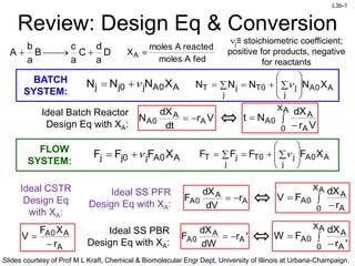
1. L3b-1
Slides courtesy of Prof M L Kraft, Chemical & Biomolecular Engr Dept, University of Illinois at Urbana-Champaign.
Ideal CSTR
Design Eq
with XA:
Review: Design Eq & Conversion
D
a
d
C
a
c
B
a
b
A 
fedAmoles
reactedAmoles
XA 
BATCH
SYSTEM: A0Aj0jj XNNN   








j
A0A
j
j0TjT XNNNN 
FLOW
SYSTEM: A0Aj0jj XFFF   








j
A0A
j
j0TjT XFFFF 
r
XF
V
A
A0A


Vr
dt
dX
N A
A
0A 
Ideal Batch Reactor
Design Eq with XA:



AX
0 A
A
0A
Vr
dX
Nt
A
A
0A r
dV
dX
F 
Ideal SS PFR
Design Eq with XA:



AX
0 A
A
0A
r
dX
FV
'r
dW
dX
F A
A
0A 
Ideal SS PBR
Design Eq with XA:



AX
0 A
A
0A
'r
dX
FW
j≡ stoichiometric coefficient;
positive for products, negative
for reactants

2. L3b-2
Slides courtesy of Prof M L Kraft, Chemical & Biomolecular Engr Dept, University of Illinois at Urbana-Champaign.
Review: Sizing CSTRsWe can determine the volume of the CSTR required to achieve a specific
conversion if we know how the reaction rate rj depends on the conversion Xj
A
A
0A
CSTR
A
A0A
CSTR X
r
F
V
r
XF
V 









Ideal SS
CSTR
design eq.
Volume is
product of FA0/-rA
and XA
• Plot FA0/-rA vs XA (Levenspiel plot)
• VCSTR is the rectangle with a base of XA,exit and a height of FA0/-rA at XA,exit

FA 0
rA
X
Area = Volume of CSTR
X1
V 
FA 0
rA



X1
 X1

3. L3b-3
Slides courtesy of Prof M L Kraft, Chemical & Biomolecular Engr Dept, University of Illinois at Urbana-Champaign.
FA 0
rA
Area = Volume of PFR
V 
0
X1

FA 0
rA





dX
X1
Area = VPFR or Wcatalyst, PBR
dX
'r
F
W
1X
0 A
0A
 







Review: Sizing PFRs & PBRs
We can determine the volume (catalyst weight) of a PFR (PBR) required to
achieve a specific Xj if we know how the reaction rate rj depends on Xj
A
exit,AX
0 A
0A
PFR
exit,AX
0 A
A
0APFR dX
r
F
V
r
dX
FV  









Ideal PFR
design eq.
• Plot FA0/-rA vs XA (Experimentally determined numerical values)
• VPFR (WPBR) is the area under the curve FA0/-rA vs XA,exit
A
exit,AX
0 A
0A
PBR
exit,AX
0 A
A
0APBR dX
r
F
W
r
dX
FW  








Ideal PBR
design eq.
dX
r
F
V
1X
0 A
0A
 








4. L3b-4
Slides courtesy of Prof M L Kraft, Chemical & Biomolecular Engr Dept, University of Illinois at Urbana-Champaign.
Numerical Evaluation of Integrals (A.4)
Simpson’s one-third rule (3-point):
        210
2X
0
XfXf4Xf
3
h
dxxf 
hXX
2
XX
h 01
02 


Trapezoidal rule (2-point):
      10
1X
0
XfXf
2
h
dxxf 
01 XXh 
Simpson’s three-eights rule (4-point):
          3210
3X
0
XfXf3Xf3Xfh
8
3
dxxf 
3
XX
h 03 

h2XXhXX 0201 
Simpson’s five-point quadrature :
            43210
4X
0
XfXf4Xf2Xf4Xf
3
h
dxxf 
4
XX
h 04 


5. L3b-5
Slides courtesy of Prof M L Kraft, Chemical & Biomolecular Engr Dept, University of Illinois at Urbana-Champaign.
Review: Reactors in Series
2 CSTRs 2 PFRs
CSTR→PFR
VCSTR1 VPFR2
VPFR2VCSTR1
VCSTR2
VPFR1
VPFR1
VCSTR2
VCSTR1 + VPFR2
≠
VPFR1 + CCSTR2
PFR→CSTR
A
A0
r-
F
 
i j
CSTRPFRPFR VVV
If is monotonically
increasing then:
CSTR
i j
CSTRPFR VVV  

6. L3b-6
Slides courtesy of Prof M L Kraft, Chemical & Biomolecular Engr Dept, University of Illinois at Urbana-Champaign.
Chapter 2 Examples

7. L3b-7
Slides courtesy of Prof M L Kraft, Chemical & Biomolecular Engr Dept, University of Illinois at Urbana-Champaign.
XA 0 0.1 0.2 0.3 0.4 0.5 0.6 0.7 0.8 0.85
-rA 0.0053 0.0052 0.0050 0.0045 0.0040 0.0033 0.0025 0.0018 0.00125 0.001
1. Calculate FA0/-rA for each conversion value in the tableFA0/-rA
Calculate the reactor volumes for each configuration shown below for the reaction data
in the table when the molar flow rate is 52 mol/min.
FA0, X0
X1=0.3
X2=0.8
Config 1
X1=0.3
FA0, X0 X2=0.8
Config 2
A
exit,AX
in,AX A
0A
nPFR dX
r
F
V  






 ←Use numerical
methods to solve
 in,Aout,A
nA
0A
nCSTR XX
r
F
V 


XA,out and XA,in respectively, are the conversion at the outlet and inlet of reactor n
Convert to seconds→
min
mol
52F 0A 
00
1
52 8
60
67
 
 
 
 A
mol min
m
mol
. F
sin s
-rA is in terms of mol/dm3∙s

8. L3b-8
Slides courtesy of Prof M L Kraft, Chemical & Biomolecular Engr Dept, University of Illinois at Urbana-Champaign.
A(
0
0)
AF
r

3
3
mol
0.0053
d
mol
0.867
s
s
m
m
d

164
1. Calculate FA0/-rA for each conversion value in the table
XA 0 0.1 0.2 0.3 0.4 0.5 0.6 0.7 0.8 0.85
-rA 0.0053 0.0052 0.0050 0.0045 0.0040 0.0033 0.0025 0.0018 0.00125 0.001
FA0/-rA 164
Calculate the reactor volumes for each configuration shown below for the reaction data
in the table when the molar flow rate is 52 mol/min.
FA0, X0
X1=0.3
X2=0.8
Config 1
X1=0.3
FA0, X0 X2=0.8
Config 2
A
exit,AX
in,AX A
0A
nPFR dX
r
F
V  






 ←Use numerical
methods to solve
 in,Aout,A
nA
0A
nCSTR XX
r
F
V 


-rA is in terms of mol/dm3∙s
164
XA,out and XA,in respectively, are the conversion at the outlet and inlet of reactor n
min
mol
52F 0A 
00
1
52 8
60
67
 
 
 
 A
mol min
m
mol
. F
sin s
Convert to seconds→

9. L3b-9
Slides courtesy of Prof M L Kraft, Chemical & Biomolecular Engr Dept, University of Illinois at Urbana-Champaign.
A(
0
0)
AF
r

3
3
mol
0.0053
d
mol
0.867
s
s
m
m
d

164
1. Calculate FA0/-rA for each conversion value in the table
XA 0 0.1 0.2 0.3 0.4 0.5 0.6 0.7 0.8 0.85
-rA 0.0053 0.0052 0.0050 0.0045 0.0040 0.0033 0.0025 0.0018 0.00125 0.001
FA0/-rA
Calculate the reactor volumes for each configuration shown below for the reaction data
in the table when the molar flow rate is 52 mol/min.
FA0, X0
X1=0.3
X2=0.8
Config 1
X1=0.3
FA0, X0 X2=0.8
Config 2
A
exit,AX
in,AX A
0A
nPFR dX
r
F
V  






 ←Use numerical
methods to solve
 in,Aout,A
nA
0A
nCSTR XX
r
F
V 


-rA is in terms of mol/dm3∙s
164
XA,out and XA,in respectively, are the conversion at the outlet and inlet of reactor n
min
mol
52F 0A 
00
1
52 8
60
67
 
 
 
 A
mol min
m
mol
. F
sin s
Convert to seconds→ For each –rA that corresponds to
a XA value, use FA0 to calculate
FA0/-rA & fill in the table

10. L3b-10
Slides courtesy of Prof M L Kraft, Chemical & Biomolecular Engr Dept, University of Illinois at Urbana-Champaign.
X1=0.3
FA0, X0
A( 0.85)
3A0
3
mol
0.867F s
molr
0.001
dm s
867 dm 


1. Calculate FA0/-rA for each conversion value in the table
XA 0 0.1 0.2 0.3 0.4 0.5 0.6 0.7 0.8 0.85
-rA 0.0053 0.0052 0.0050 0.0045 0.0040 0.0033 0.0025 0.0018 0.00125 0.001
FA0/-rA 164 167 173 193 217 263 347 482 694 867
Calculate the reactor volumes for each configuration shown below for the reaction data
in the table when the molar flow rate is 52 mol/min.
FA0, X0
X1=0.3
X2=0.8
Config 1
X2=0.8
Config 2
A
exit,AX
in,AX A
0A
nPFR dX
r
F
V  






 ←Use numerical
methods to solve
 in,Aout,A
nA
0A
nCSTR XX
r
F
V 


Convert to seconds→
min
mol
52F 0A 
-rA is in terms of mol/dm3∙s
XA,out and XA,in respectively, are the conversion at the outlet and inlet of reactor n
00
1
52 8
60
67
 
 
 
 A
mol min
m
mol
. F
sin s

11. L3b-11
Slides courtesy of Prof M L Kraft, Chemical & Biomolecular Engr Dept, University of Illinois at Urbana-Champaign.
XA 0 0.1 0.2 0.3 0.4 0.5 0.6 0.7 0.8 0.85
-rA 0.0053 0.0052 0.0050 0.0045 0.0040 0.0033 0.0025 0.0018 0.00125 0.001
FA0/-rA 164 167 173 193 217 263 347 482 694 867
FA0, X0
X1=0.3
X2=0.8
Config 1
Reactor 1, PFR from XA0=0 to XA=0.3:


 

 
   
 

        


A
A AA
A A0
A
0.3
A0
PFR1 A
0
A0
X
0
A X
A0
A
X 0.3
0.20A .X 1A 0
F 3 0.3 0
V dX 3
F F
3
rr
F
rr8 3
F
r
4-pt rule:
     1
0.3 A0
PFR A0
3
A
16
F 3
V dX 0.1 3 3 1
r 8
934 173 5167 1.6 dm         
  

A,out
2CSTR
A0
A,o A i
X
, nut
A
F
XV X
r
    2
3
CSTR 694 0.8 3470.3 dmV
Total volume for configuration 1: 51.6 dm3 + 347 dm3 = 398.6 dm3 = 399 dm3
←Use numerical
methods to solve
PFR1 CSTR2
0 
  
 

XA,exit A
PFRn AXA,in A
F
V dX
r

12. L3b-12
Slides courtesy of Prof M L Kraft, Chemical & Biomolecular Engr Dept, University of Illinois at Urbana-Champaign.
XA 0 0.1 0.2 0.3 0.4 0.5 0.6 0.7 0.8 0.85
-rA 0.0053 0.0052 0.0050 0.0045 0.0040 0.0033 0.0025 0.0018 0.00125 0.001
FA0/-rA 164 167 173 193 217 263 347 482 694 867
Reactor 1, CSTR from XA0=0 to XA=0.3:
Need to evaluate at 6 pts, but since
there is no 6-pt rule, break it up
 0
0
1 0
3
A
A .
A,outCSTR A
F
XV X
r
 

Total volume for configuration 2: 58 dm3 + 173 dm3 = 231 dm3
X1=0.3
FA0, X0 X2=0.8
Config 2
    CSTR
3
0. 583 0193 dmV  

A0
PFR2 A
A
0.8
0.3
F
V dX
r
 
     PFRV
... .                     
 
263 263 34217
3
4 3 3
8 33 2
482193 694
0 08 5
7
0 30 5
3 point rule 4 point rule
3
173 dm
PFR2CSTR1
   
 
0.
A0 A0
PF
0.3
R2 A A
A
05
.
.
5
8
A0
F F
V dX dX
r r
Must evaluate as many
pts as possible when
the curve isn’t flat

13. L3b-13
Slides courtesy of Prof M L Kraft, Chemical & Biomolecular Engr Dept, University of Illinois at Urbana-Champaign.
ACSTR
A
A
V
X
C
r
 
    
 
 0
0
CSTR
A
A
A
V
C
r
X
 
   
 
00
For a given CA0, the space time  needed to achieve 80% conversion in a
CSTR is 5 h. Determine (if possible) the CSTR volume required to process 2
ft3/min and achieve 80% conversion for the same reaction using the same CA0.
What is the space velocity (SV) for this system?
space time holding time mean residenceh
V
time

    
0
5
=5 h 0=2 ft3/min
 
ft
min h
hV
min  
      
3
60
5
2 3
V ft  600
V
SV



0 1Space
velocity:
-1
h
SV . h   

0 2
5
1 1
Notice that we did not need to solve the CSTR design equation to solve this problem.
Also, this answer does not depend on the type of flow reactor used.
XA=0.8
A
CSTR A
AF
r
XV
 
  
 
0 A
A
CSTR
A
C
r
V
X
 
  



0
0
   0
0
V
V 



14. L3b-14
Slides courtesy of Prof M L Kraft, Chemical & Biomolecular Engr Dept, University of Illinois at Urbana-Champaign.
XA,exit
PFR
A
A
X AA,in
C
V dX
r
 
    
 
 0
0
A product is produced by a nonisothermal, nonelementary, multiple-reaction
mechanism. Assume the volumetric flow rate is constant & the same in both reactors.
Data for this reaction is shown in the graph below. Use this graph to determine which
of the 2 configurations that follow give the smaller total reactor volume.
FA0, X0
X1=0.3
X2=0.7
Config 2
X1=0.3
FA0, X0 X2=0.7
Config 1
 A
CSTR A,out A,in
A
V X X
r
C 
  
 
 0
0
Shown on graph
XA,exit
PFRn A
AA,in
A
X
V dX
F
r
 
   
 
0
CSTR
A
A
A
V X
r
F 
  
 
0
• Since 0 is the same in both reactors, we can use this graph to compare the 2
configurations
• PFR- volume is 0 multiplied by the area under the curve between XA,in & XA,out
• CSTR- volume is 0 multiplied by the product of CA0/-rA,outlet times (XA,out - XA,in)

15. L3b-15
Slides courtesy of Prof M L Kraft, Chemical & Biomolecular Engr Dept, University of Illinois at Urbana-Champaign.
A product is produced by a nonisothermal, nonelementary, multiple-reaction
mechanism. Assume the volumetric flow rate is constant & the same in both reactors.
Data for this reaction is shown in the graph below. Use this graph to determine which
of the 2 configurations that follow give the smaller total reactor volume.
FA0, X0
X1=0.3
X2=0.7
Config 2
X1=0.3
FA0, X0 X2=0.7
Config 1
• PFR- V is 0 multiplied by the area under the curve between XA,in & XA,out
• CSTR- V is 0 multiplied by the product of CA0/-rA,outlet times (XA,out - XA,in)
Config 1 Config 2
Less shaded area
Config 2 (PFRXA,out=0.3 first, and CSTRXA,out=0.7 second) has the smaller VTotal
XA=0.3
XA=0.7
XA=0.3
XA=0.7