How does a neural network
work
… literally!
I mean, … really literally!
Don’t give me the formulas,
Don’t give me the python code
JUST GIVE ME THE NUMBERS!
Ok, here it is ….
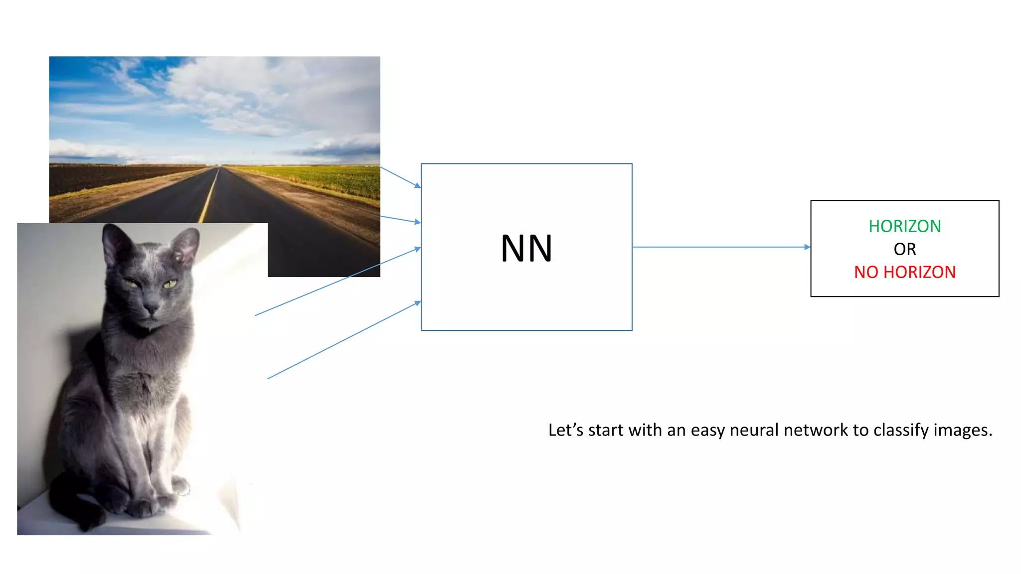
NN
HORIZON
OR
NO HORIZON
Let’s start with an easy neural network to classify images.
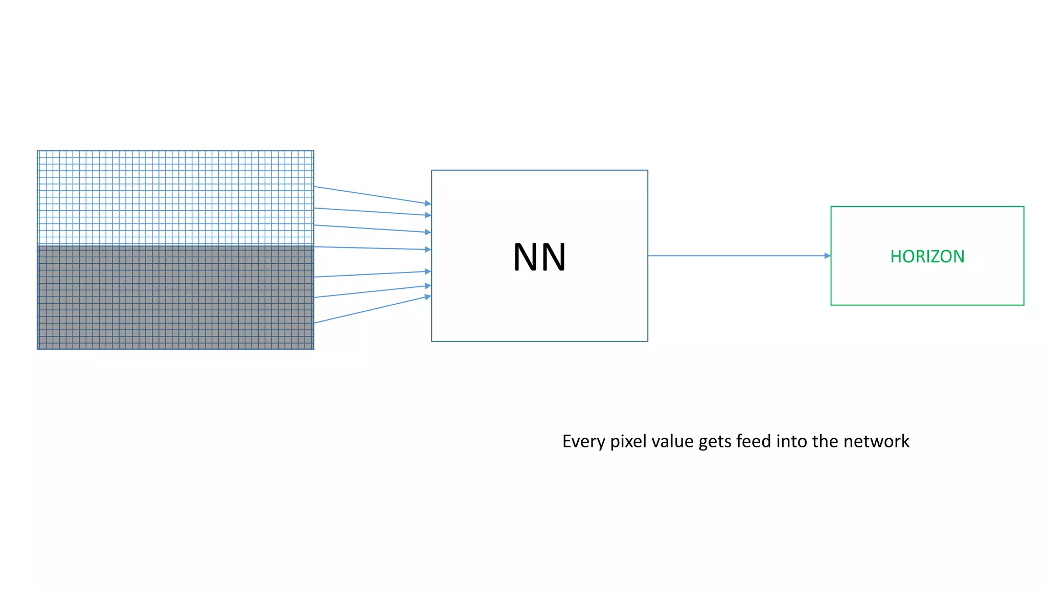
NN HORIZON
Every pixel value gets feed into the network
HORIZON
At Wikipedia you find images like these, which show, that
Every pixel value is feed into every neuron.
Looks complicated! But the math is actually not that hard.
It’ just a lot of calculations! So let’s break it down.
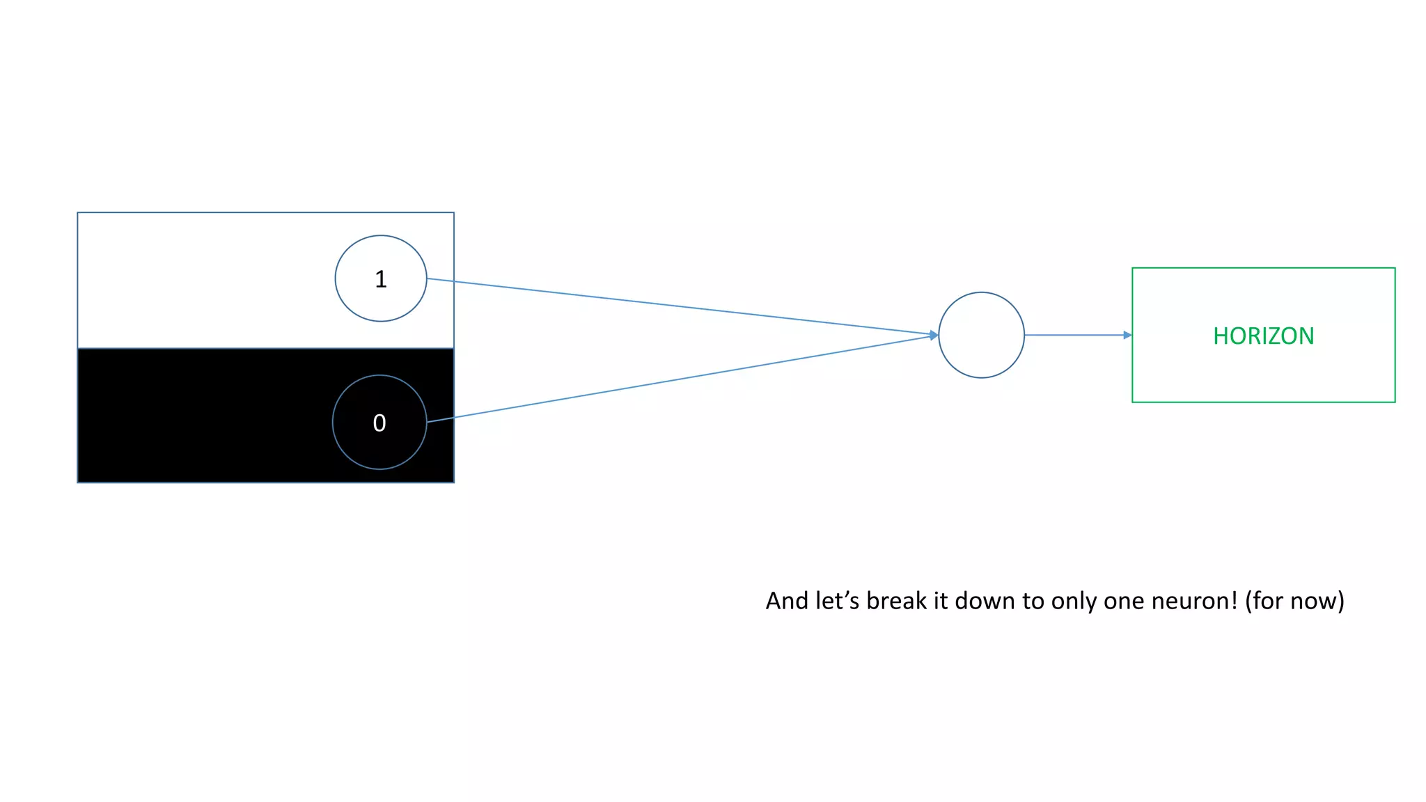
HORIZON
1
0
Let’s focus on images with two pixels only. (for now)
HORIZON
1
0
And let’s break it down to only one neuron! (for now)
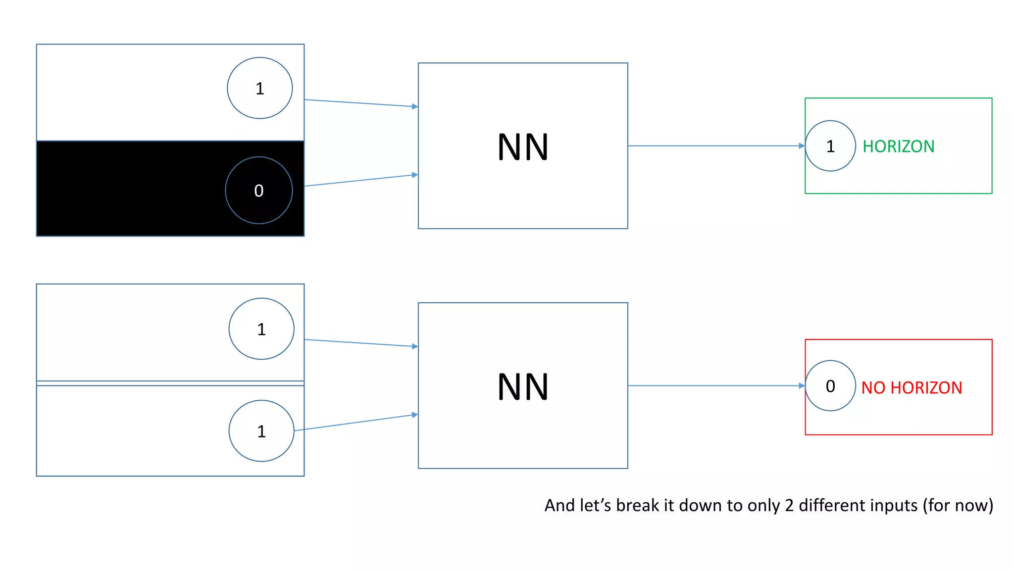
1
0
1
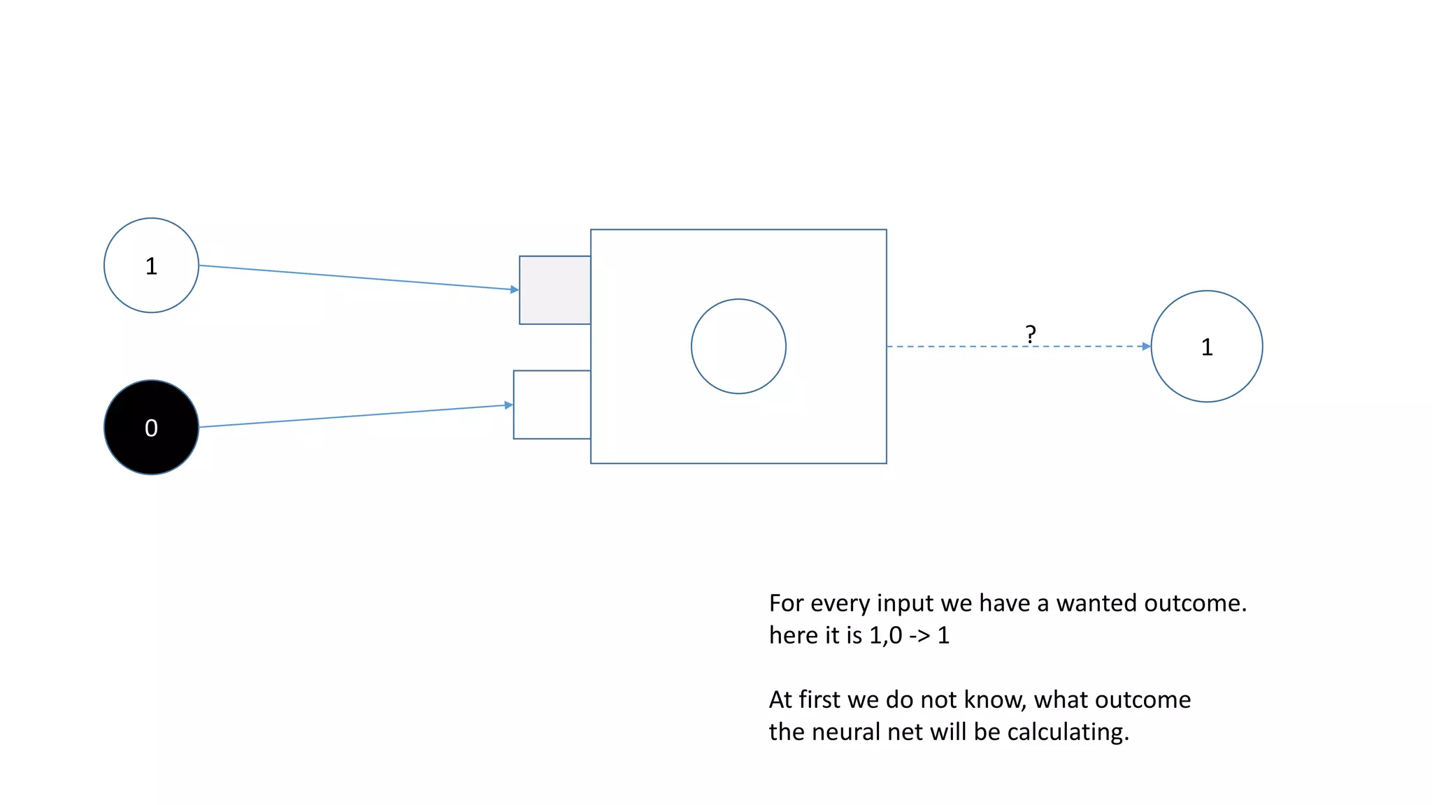
For every input we have a wanted outcome.
here it is 1,0 -> 1
At first we do not know, what outcome
the neural net will be calculating.
?
1
0
1
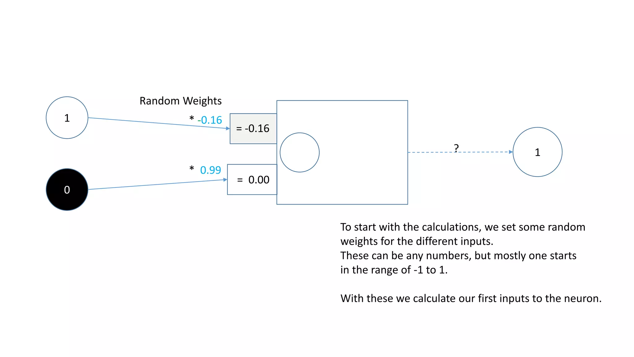
* -0.16
* 0.99
Random Weights
To start with the calculations, we set some random
weights for the different inputs.
These can be any numbers, but mostly one starts
in the range of -1 to 1.
With these we calculate our first inputs to the neuron.
?
= -0.16
= 0.00
1
0
1
* -0.16
* 0.99
Random Weights
Then we add up the results for every weight.
?
= -0.16
= 0.00
+ -0.16
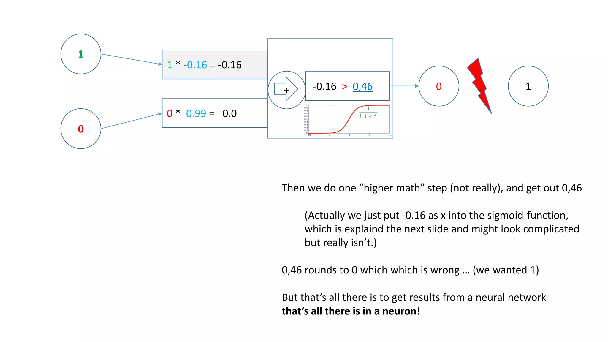
1 * -0.16 = -0.16
0 * 0.99 = 0.0
1
0
+ -0.16 > 0,46 0 1
Then we do one “higher math” step (not really), and get out 0,46
(Actually we just put -0.16 as x into the sigmoid-function,
which is explaind the next slide and might look complicated
but really isn’t.)
0,46 rounds to 0 which which is wrong … (we wanted 1)
But that’s all there is to get results from a neural network
that’s all there is in a neuron!
1 * -0.16 = -0.16
0 * 0.99 = 0.0
1
0
+ -0.16 > 0,46 0 1
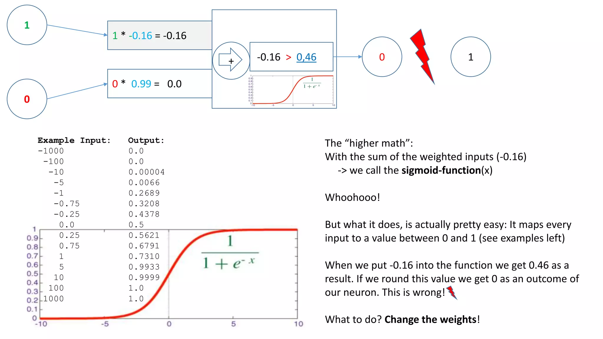
Example Input: Output:
-1000 0.0
-100 0.0
-10 0.00004
-5 0.0066
-1 0.2689
-0.75 0.3208
-0.25 0.4378
0.0 0.5
0.25 0.5621
0.75 0.6791
1 0.7310
5 0.9933
10 0.9999
100 1.0
1000 1.0
The “higher math”:
With the sum of the weighted inputs (-0.16)
-> we call the sigmoid-function(x)
Whoohooo!
But what it does, is actually pretty easy: It maps every
input to a value between 0 and 1 (see examples left)
When we put -0.16 into the function we get 0.46 as a
result. If we round this value we get 0 as an outcome of
our neuron. This is wrong!
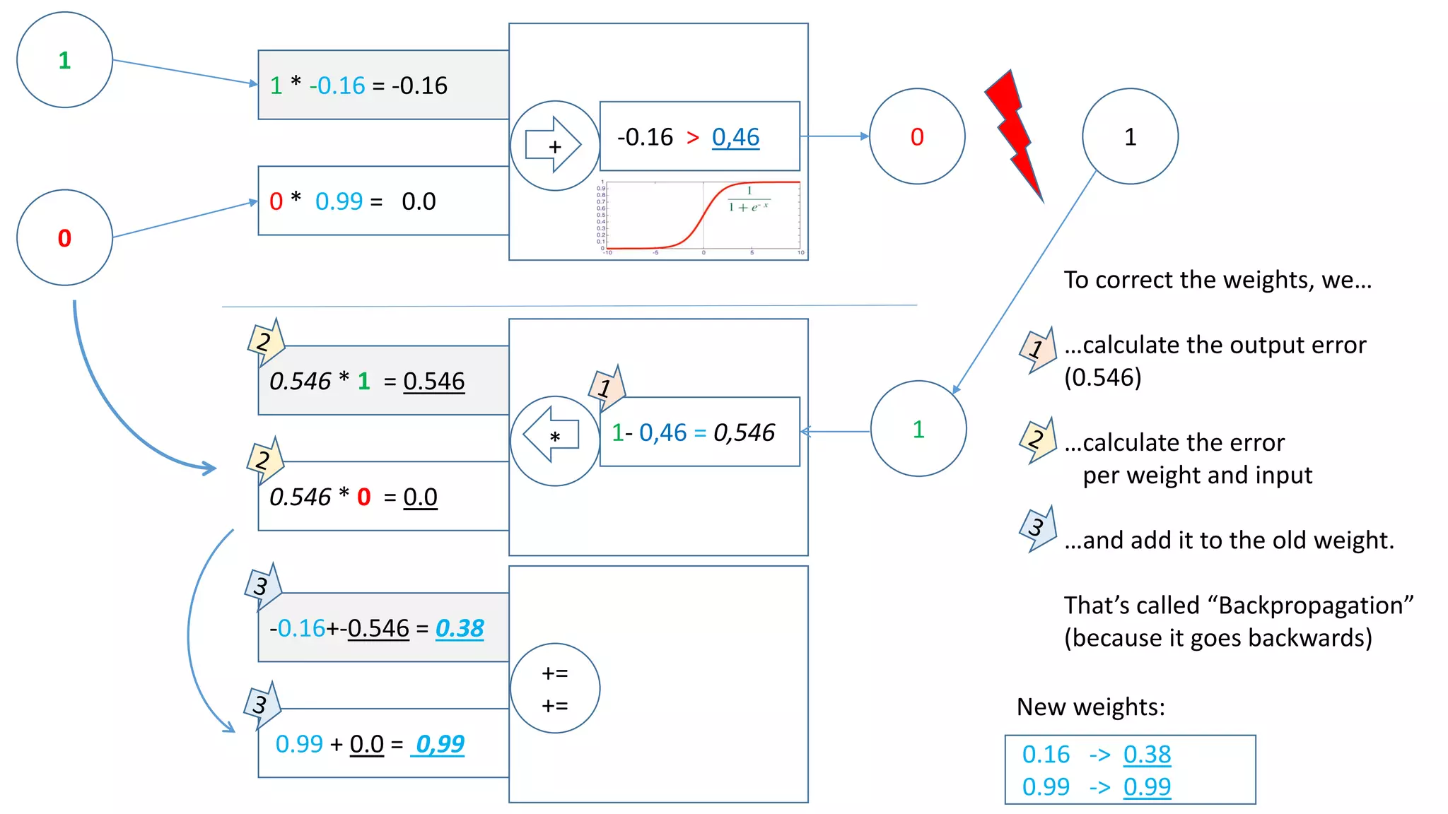
What to do? Change the weights!
1 * -0.16 = -0.16
0 * 0.99 = 0.0
1
0
+ -0.16 > 0,46 0
0.546 * 1 = 0.546
0.546 * 0 = 0.0
* 1- 0,46 = 0,546 1
1
-0.16+-0.546 = 0.38
0.99 + 0.0 = 0,99
+=
+=
0.16 -> 0.38
0.99 -> 0.99
New weights:
To correct the weights, we…
…calculate the output error
(0.546)
…calculate the error
per weight and input
…and add it to the old weight.
That’s called “Backpropagation”
(because it goes backwards)
1 * 0.38 = 0.38
0 * 0.99 = 0.0
+ 0.38 > 0,59 1
1
0
AND THAT‘s IT!
Well… basically it really is.
It‘s all about getting input values to the right output values
by adjusting the weights.
But obviously neural nets have more than one neuron.
And normally there is more than one input.
Let‘s increase the input‘s first!
Now we calculate again, and get the right output!
1
1
0
1
0
1
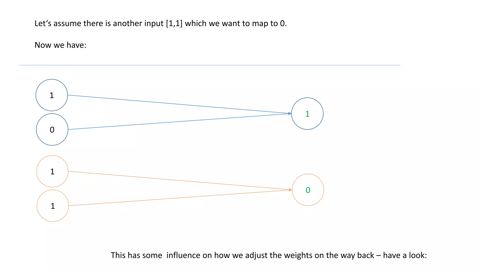
Let‘s assume there is another input [1,1] which we want to map to 0.
Now we have:
This has some influence on how we adjust the weights on the way back – have a look:
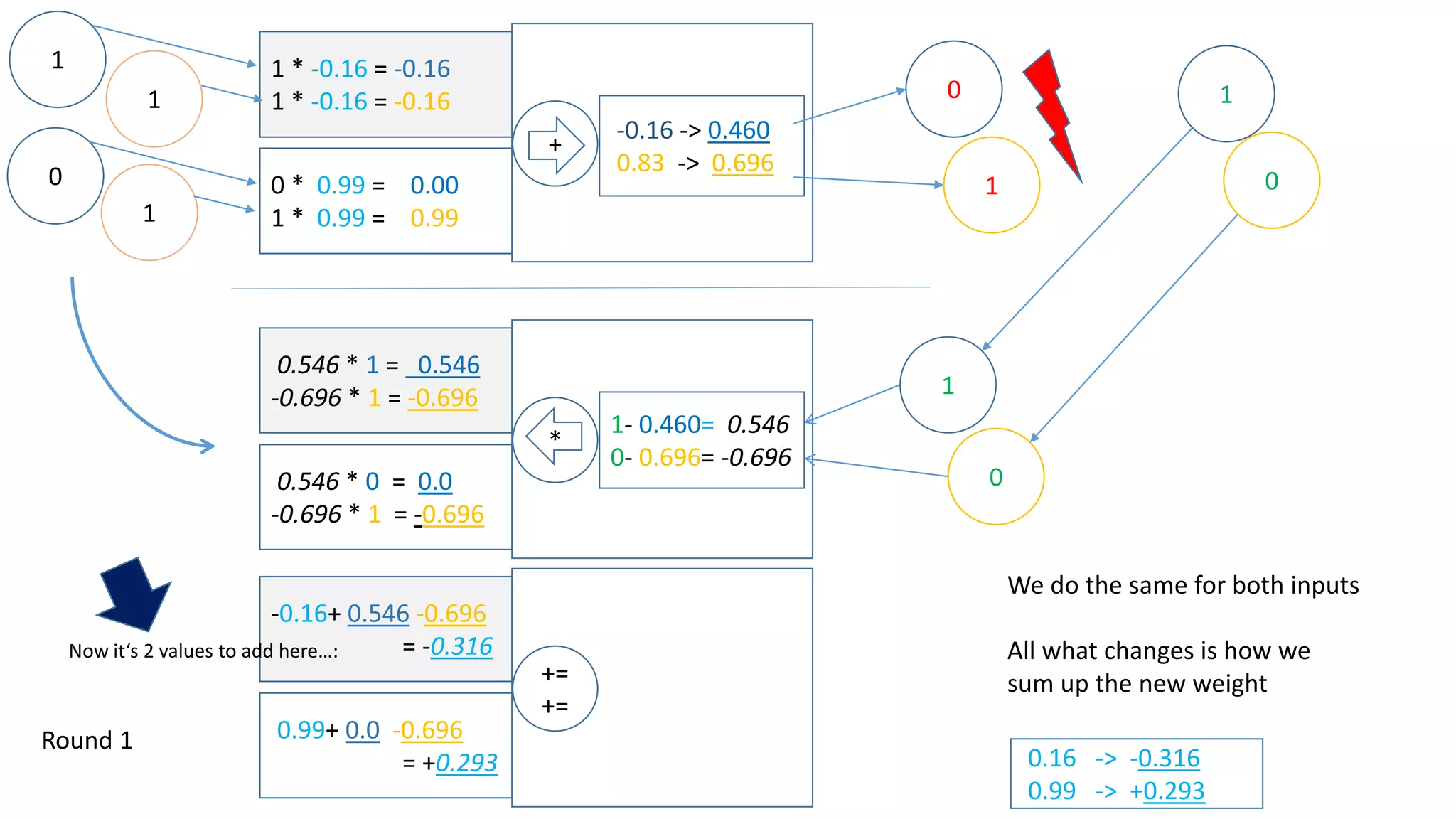
1 * -0.16 = -0.16
1 * -0.16 = -0.16
0 * 0.99 = 0.00
1 * 0.99 = 0.99
1
0
+
-0.16 -> 0.460
0.83 -> 0.696
0
0.546 * 1 = 0.546
-0.696 * 1 = -0.696
0.546 * 0 = 0.0
-0.696 * 1 = -0.696
*
1- 0.460= 0.546
0- 0.696= -0.696
1
-0.16+ 0.546 -0.696
= -0.316
0.99+ 0.0 -0.696
= +0.293
+=
+=
1
1
1 0
0
1
0.16 -> -0.316
0.99 -> +0.293
Round 1
Now it‘s 2 values to add here…:
We do the same for both inputs
All what changes is how we
sum up the new weight
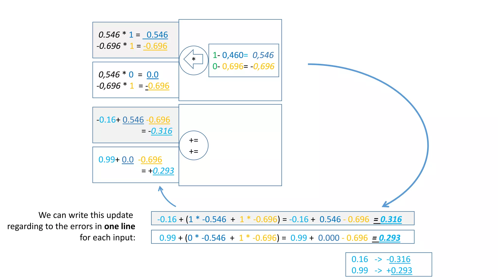
-0.16 + (1 * -0.546 + 1 * -0.696) = -0.16 + 0.546 - 0.696 = -0.316
We can write this update regarding to the errors
in one line for each input weight:
0.99 + (0 * -0.546 + 1 * -0.696) = 0.99 + 0.000 - 0.696 = 0.293
0.16 -> -0.316
0.99 -> +0.293
0.546 * 1 = 0.546
-0.696 * 1 = -0.696
0.546 * 0 = 0.0
-0.696 * 1 = -0.696
*
1- 0.460= 0.546
0- 0.696= -0.696
-0.16+ 0.546 -0.696
= -0.316
0.99+ 0.0 -0.696
= +0.293
+=
+=
(we will do this again later when we have many weights…)
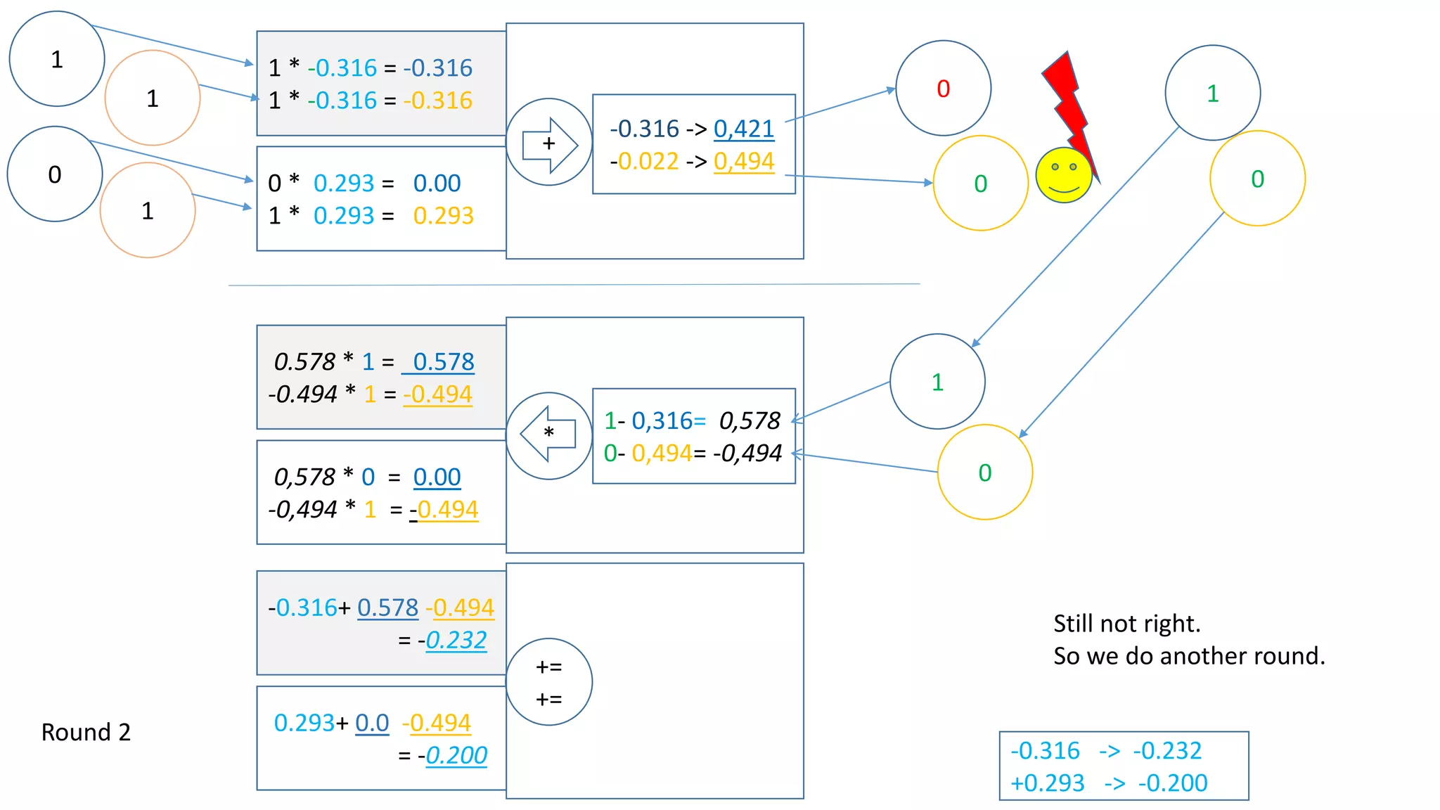
1 * -0.316 = -0.316
1 * -0.316 = -0.316
0 * 0.293 = 0.00
1 * 0.293 = 0.293
1
0
+
-0.316 -> 0,421
-0.022 -> 0,494
0
0.578 * 1 = 0.578
-0.494 * 1 = -0.494
0,578 * 0 = 0.00
-0,494 * 1 = -0.494
*
1- 0,421= 0,578
0- 0,494= -0,494
1
-0.316+ 0.578 -0.494
= -0.232
0.293+ 0.0 -0.494
= -0.200
+=
+=
1
1
0 0
0
1
-0.316 -> -0.232
+0.293 -> -0.200
Round 2
Still not right.
So we do another round.
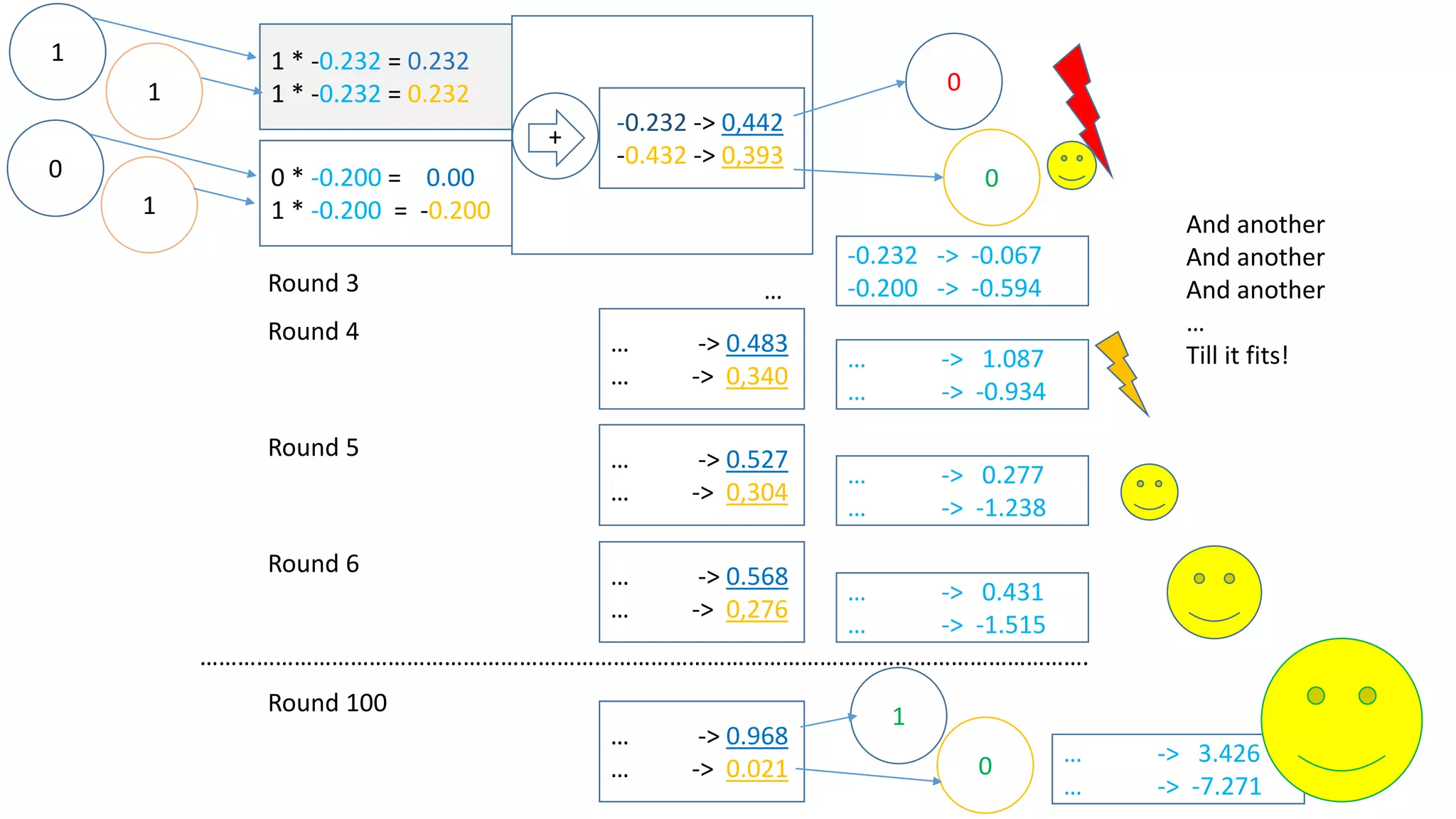
1 * -0.232 = 0.232
1 * -0.232 = 0.232
0 * -0.200 = 0.00
1 * -0.200 = -0.200
1
0
+
-0.232 -> 0,442
-0.432 -> 0,393
01
1
0
-0.232 -> -0.067
-0.200 -> -0.594…
… -> 1.087
… -> -0.934
… -> 0.483
… -> 0,340
… -> 0.277
… -> -1.238
… -> 0.527
… -> 0,304
… -> 0.568
… -> 0,276
… -> 0.431
… -> -1.515
… -> 0.968
… -> 0.021
… -> 3.426
… -> -7.271
Round 4
Round 3
Round 5
Round 6
Round 100
…………………………………………………………………………………………………………………………….
1
0
And another
And another
And another
…
Till it fits!
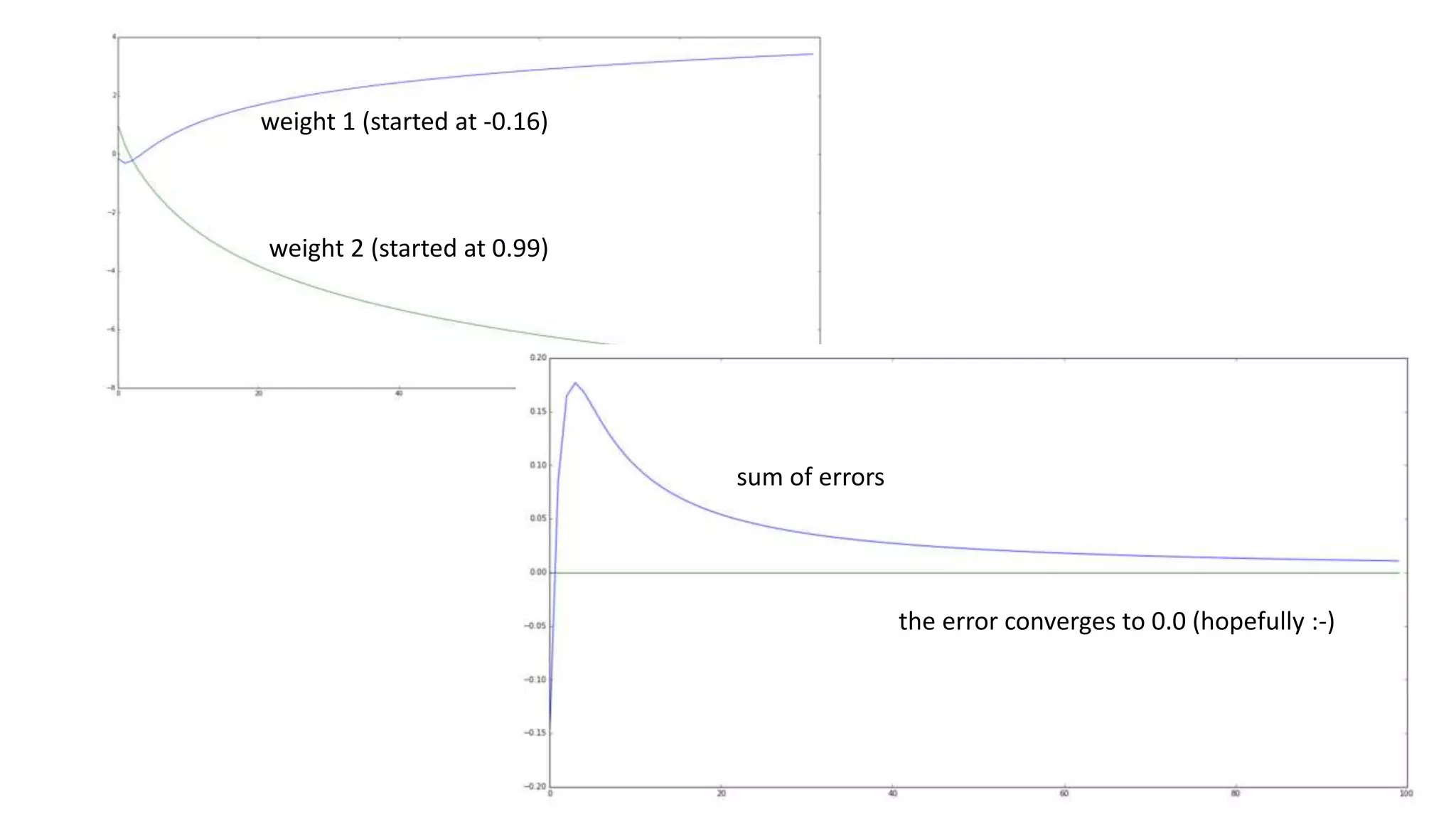
weight 1 (started at -0.16)
weight 2 (started at 0.99)
sum of errors
the error converges to 0.0 (hopefully :-)
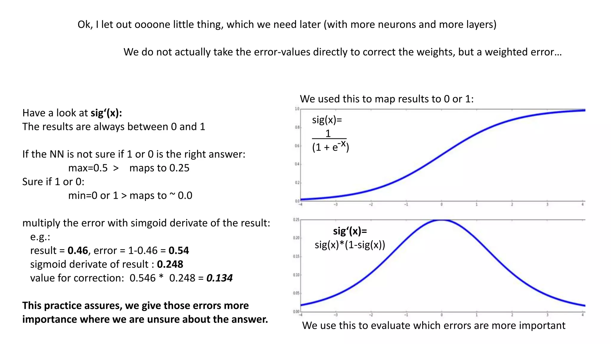
Ok, I let out oooone little thing, which we need later (with more neurons and more layers)
We do not actually take the error-values directly to correct the weights, but a weighted error…
Have a look at sig‘(x):
The results are always between 0 and 1
If the NN is not sure if 1 or 0 is the right answer:
max=0.5 > maps to 0.25
Sure if 1 or 0:
min=0 or 1 > maps to ~ 0.0
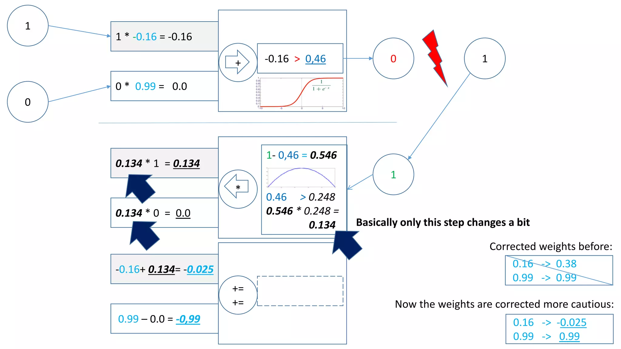
multiply the error with simgoid derivate of the result:
e.g.:
result = 0.46, error = 1-0.46 = 0.54
sigmoid derivate of result : 0.248
value for correction: 0.546 * 0.248 = 0.134
This practice assures, we give those errors more
importance where we are unsure about the answer.
sig‘(x)=
sig(x)*(1-sig(x))
sig(x)=
1
(1 + e )-x
We used this to map results to 0 or 1:
We use this to evaluate which errors are more important
1 * -0.16 = -0.16
0 * 0.99 = 0.0
1
0
+ -0.16 > 0,46 0
0.134 * 1 = 0.134
0.134 * 0 = 0.0
*
1- 0,46 = 0.546
0.46 > 0.248
0.546 * 0.248 =
0.134
1
1
-0.16+ 0.134= -0.025
0.99 – 0.0 = -0,99
+=
+=
0.16 -> -0.025
0.99 -> 0.99
Now the weights are corrected more cautious:
0.16 -> 0.38
0.99 -> 0.99
Corrected weights before:
Basically only this number changes a bit
1 * -0.16 = -0.16
0 * 0.99 = 0.0
1
0
+ -0.16 > 0,46 0
0.546 * 1 = 0.546
0.546 * 0 = 0.0
* 1- 0,46 = 0,546
1
1
-0.16+-0.546 = 0.38
0.99 + 0.0 = 0,99
+=
+=
0.16 -> 0.38
0.99 -> 0.99
New weights:
To correct the weights, we…
…calculate the output error
(0.546)
…calculate the error
per weight and input
…and add it to the old weight.
That’s called “Backpropagation”
(because it goes backwards)
(s. slide 12)
This was fun – let’s try another more complicated example with our neuron
…. XOR
0
0
0
0
1
1
1
0
1
1
1
0
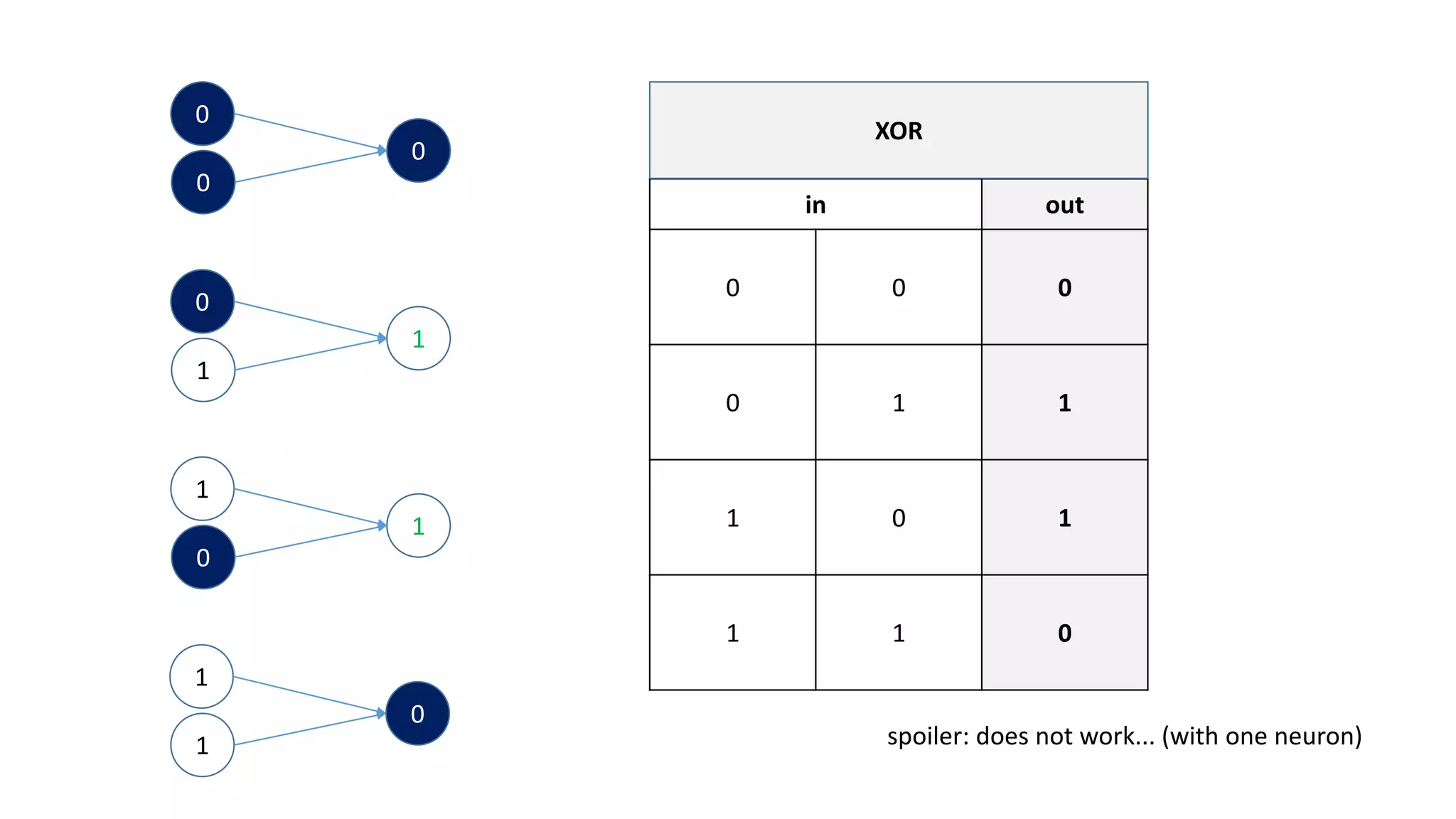
in out
0 0 0
0 1 1
1 0 1
1 1 0
XOR
spoiler: does not work... (with one neuron)
sum of error == 0!
But…:
[0,0] -> out = 0.5 -> error = -0.5
[0,1] -> out = 0.5 -> error = 0.5
[1,0] -> out = 0.5 -> error = 0.5
[1,1] -> out = 0.5 -> error = -0.5
The weights are actually both 0!
If you think about it, it‘s pretty obvious.
Every weight has to be the same, because
a 1 or 0 leads to 0 or 1
in the same amount of cases
For XOR to work we need more layers!
0
1
1
?
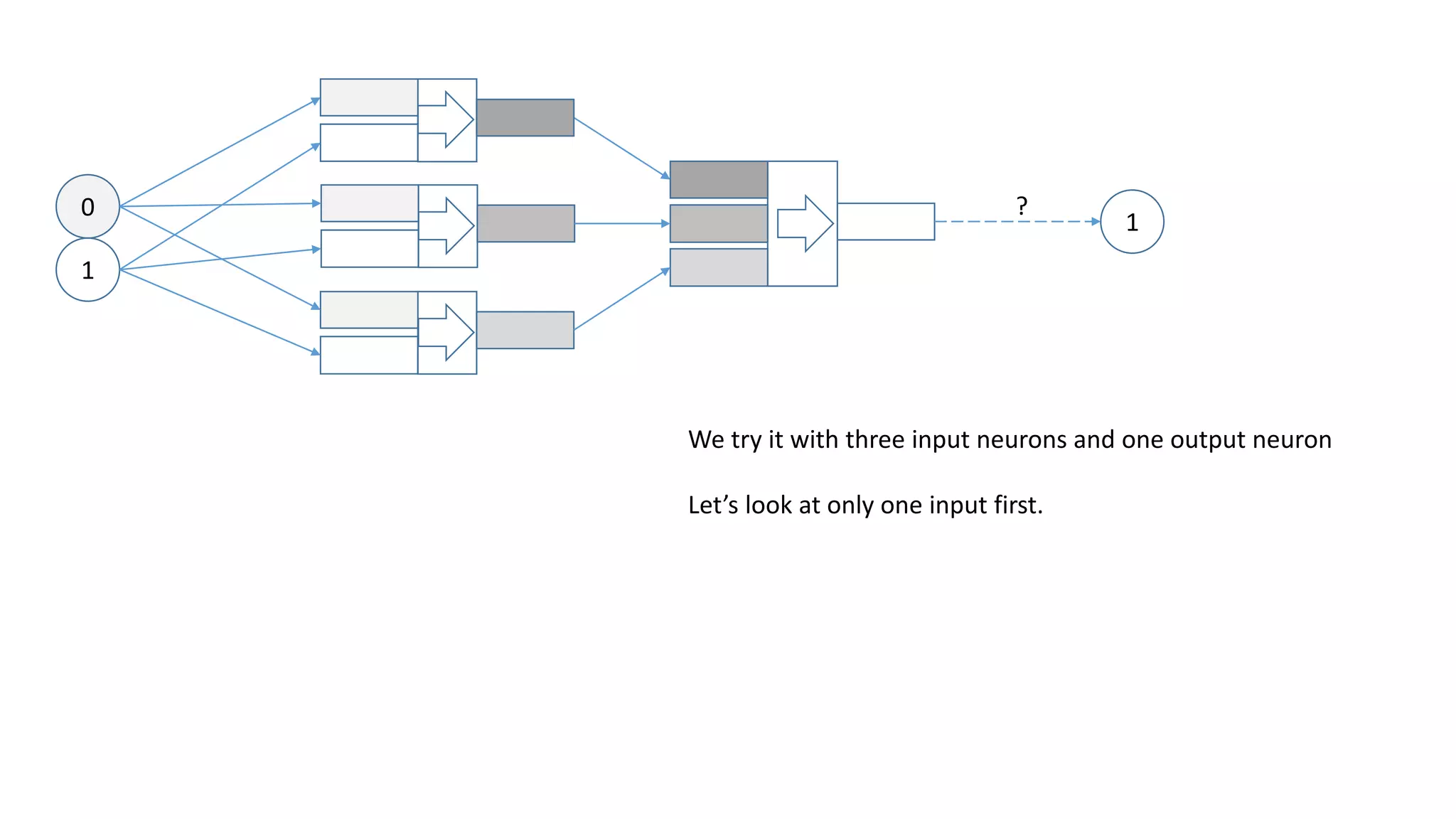
We try it with three input neurons and one output neuron
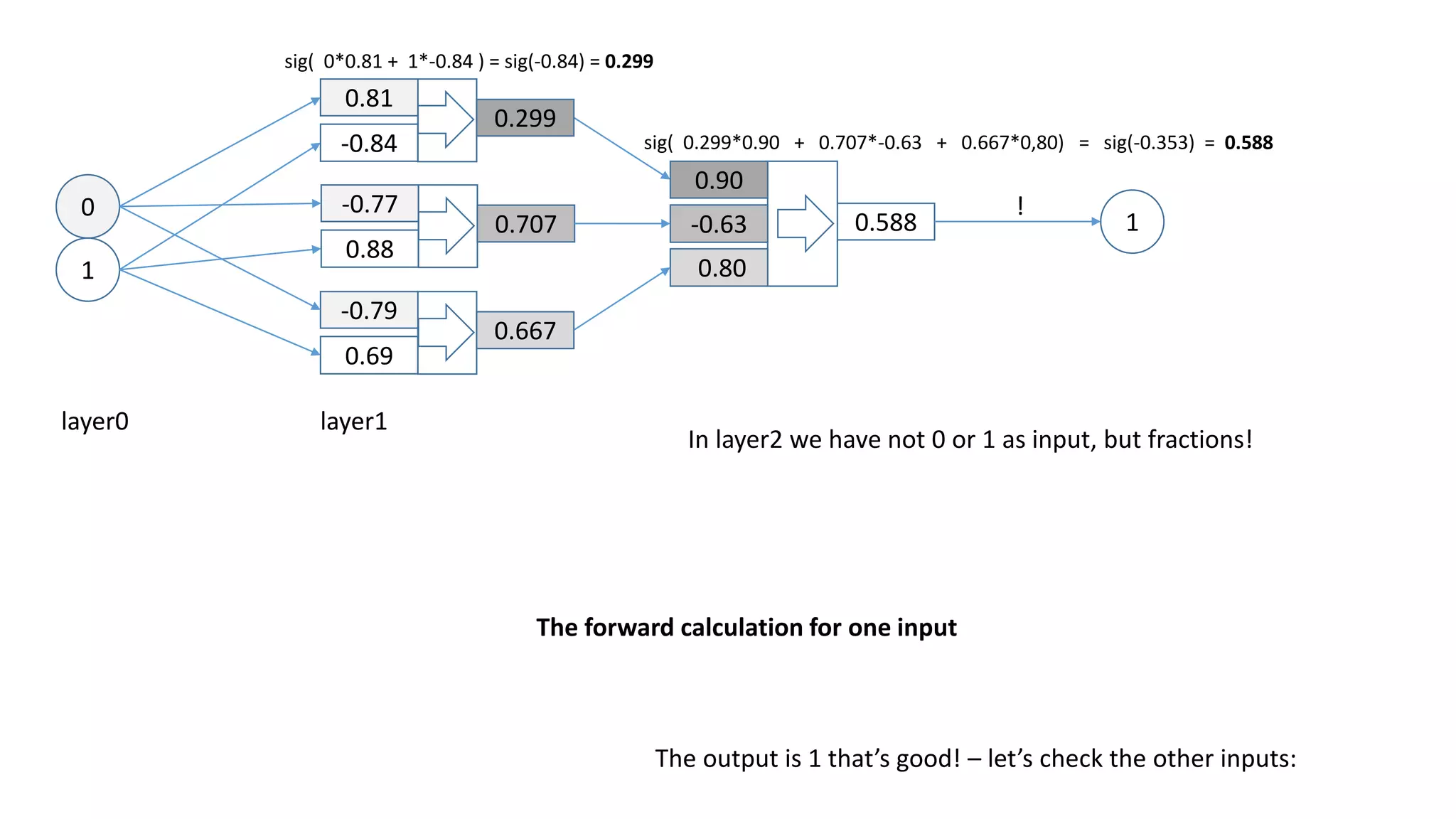
Let’s look at only one input first.
0
1
0.81
-0.84
0.299
0.90
-0.63 0.588
-0.77
0.88
0.707
-0.79
0.69
0.667
0.80
sig( 0*0.81 + 1*-0.84 ) = sig(-0.84) = 0.299
sig( 0.299*0.90 + 0.707*-0.63 + 0.667*0,80) = sig(-0.353) = 0.588
The forward calculation for one input
The output is 1 that’s good! – let’s check the other inputs:
layer0 layer1
In layer2 we have not 0 or 1 as input, but fractions!
1
!
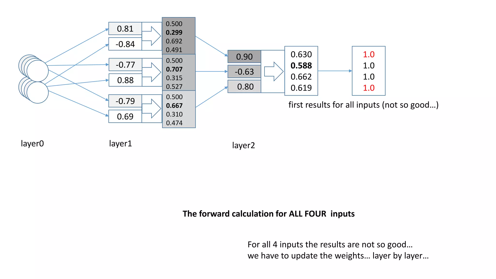
layer2layer0 layer1
0.81
-0.84
0.500
0.299
0.692
0.491
0.90
-0.63
0.630
0.588
0.662
0.619
-0.77
0.88
-0.79
0.69
0.80
0.500
0.707
0.315
0.527
0.500
0.667
0.310
0.474
first results for all inputs (not so good…)
The forward calculation for ALL FOUR inputs
1.0
1.0
1.0
1.0
For all 4 inputs the results are not so good…
we have to update the weights… layer by layer…
0.81
-0.84
0.84
-0.69-0.77
0.88
-0.79
0.69
0.75
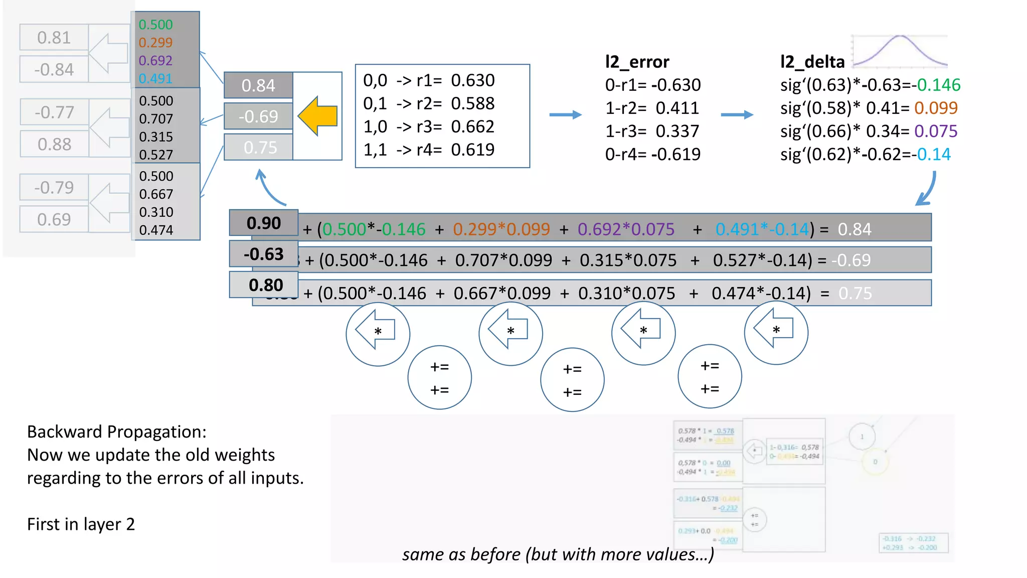
l2_error
0-r1= -0.630
1-r2= 0.411
1-r3= 0.337
0-r4= -0.619
l2_delta
sig‘(0.63)*-0.63=-0.146
sig‘(0.58)* 0.41= 0.099
sig‘(0.66)* 0.34= 0.075
sig‘(0.62)*-0.62=-0.14
0.90 + (0.500*-0.146 + 0.299*0.099 + 0.692*0.075 + 0.491*-0.14) = 0.84
-0.63 + (0.500*-0.146 + 0.707*0.099 + 0.315*0.075 + 0.527*-0.14) = -0.69
0.80 + (0.500*-0.146 + 0.667*0.099 + 0.310*0.075 + 0.474*-0.14) = 0.75
same as before (but with more values…)
0.500
0.299
0.692
0.491
0.500
0.707
0.315
0.527
0.500
0.667
0.310
0.474
* * * *
+=
+=
+=
+=
+=
+=
0,0 -> r1= 0.630
0,1 -> r2= 0.588
1,0 -> r3= 0.662
1,1 -> r4= 0.619
Backward Propagation:
Now we update the old weights
regarding to the errors of all inputs.
First in layer 2
0.90
-0.63
0.80
0.795
-0.861
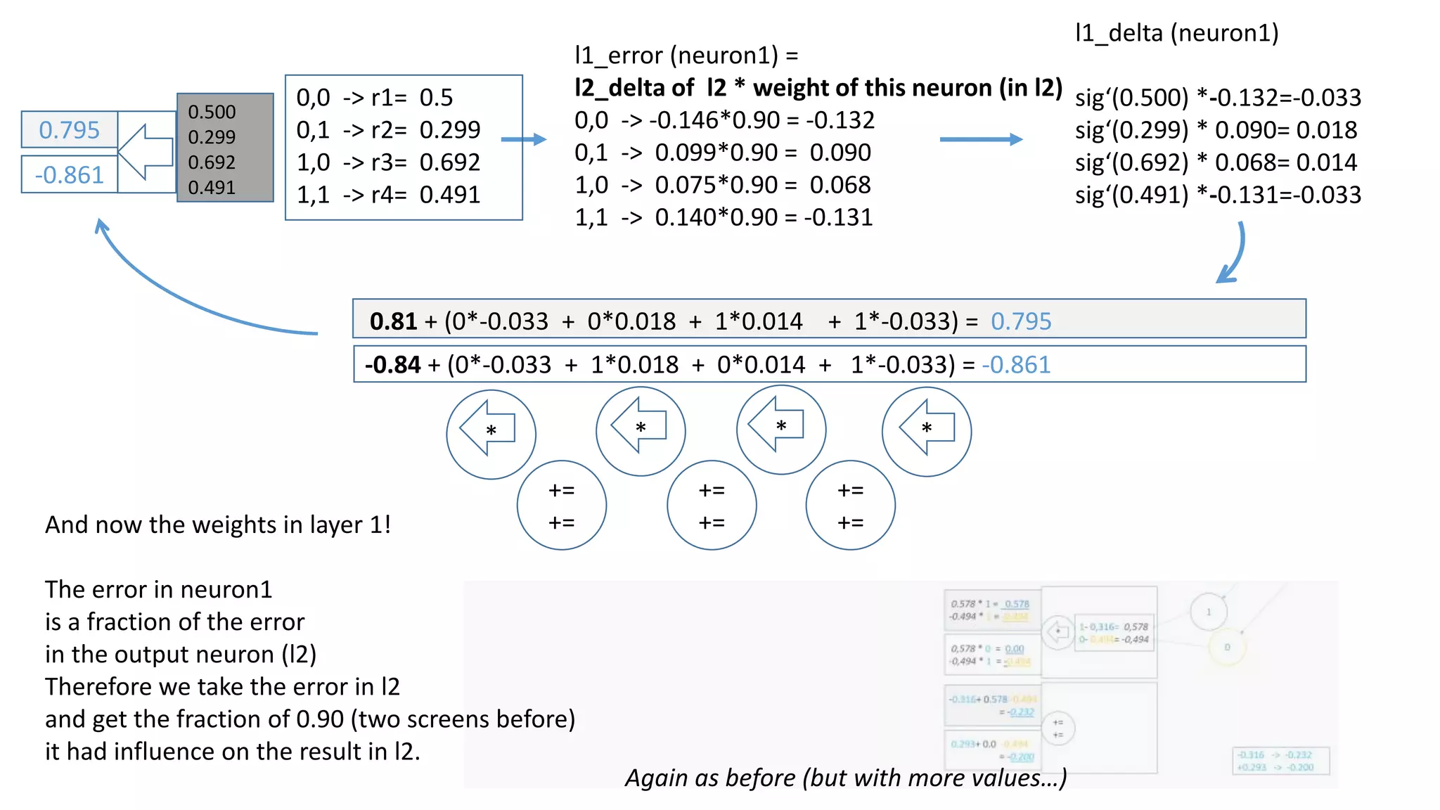
0.81 + (0*-0.033 + 0*0.018 + 1*0.014 + 1*-0.033) = 0.795
-0.84 + (0*-0.033 + 1*0.018 + 0*0.014 + 1*-0.033) = -0.861
Again as before (but with more values…)
0.500
0.299
0.692
0.491
* * *
+=
+=
+=
+=
0,0 -> r1= 0.5
0,1 -> r2= 0.299
1,0 -> r3= 0.692
1,1 -> r4= 0.491
l1_delta
sig‘(0.500) *-0.132 =-0.033
sig‘(0.299) * 0.090 = 0.018
sig‘(0.692) * 0.068 = 0.014
sig‘(0.491) *-0.131 =-0.033
l1_error =
l2_delta * weight of neuron 1 (to l2)
0,0 -> -0.146*0.90 = -0.132
0,1 -> 0.099*0.90 = 0.090
1,0 -> 0.075*0.90 = 0.068
1,1 -> 0.140*0.90 = -0.131
And now the weights in layer 1!
The error in neuron1
is a fraction of the error
in the output neuron (l2)
Therefore we take the delta-error of layer2;
neuron1 accounted 0.90 to this error:
l2_delta * weight of neuron 1 to l2
And of this we get the delta again -> l1_delta
*
+=
+=
0.81
-0.84
Neuron 1 in layer 1:
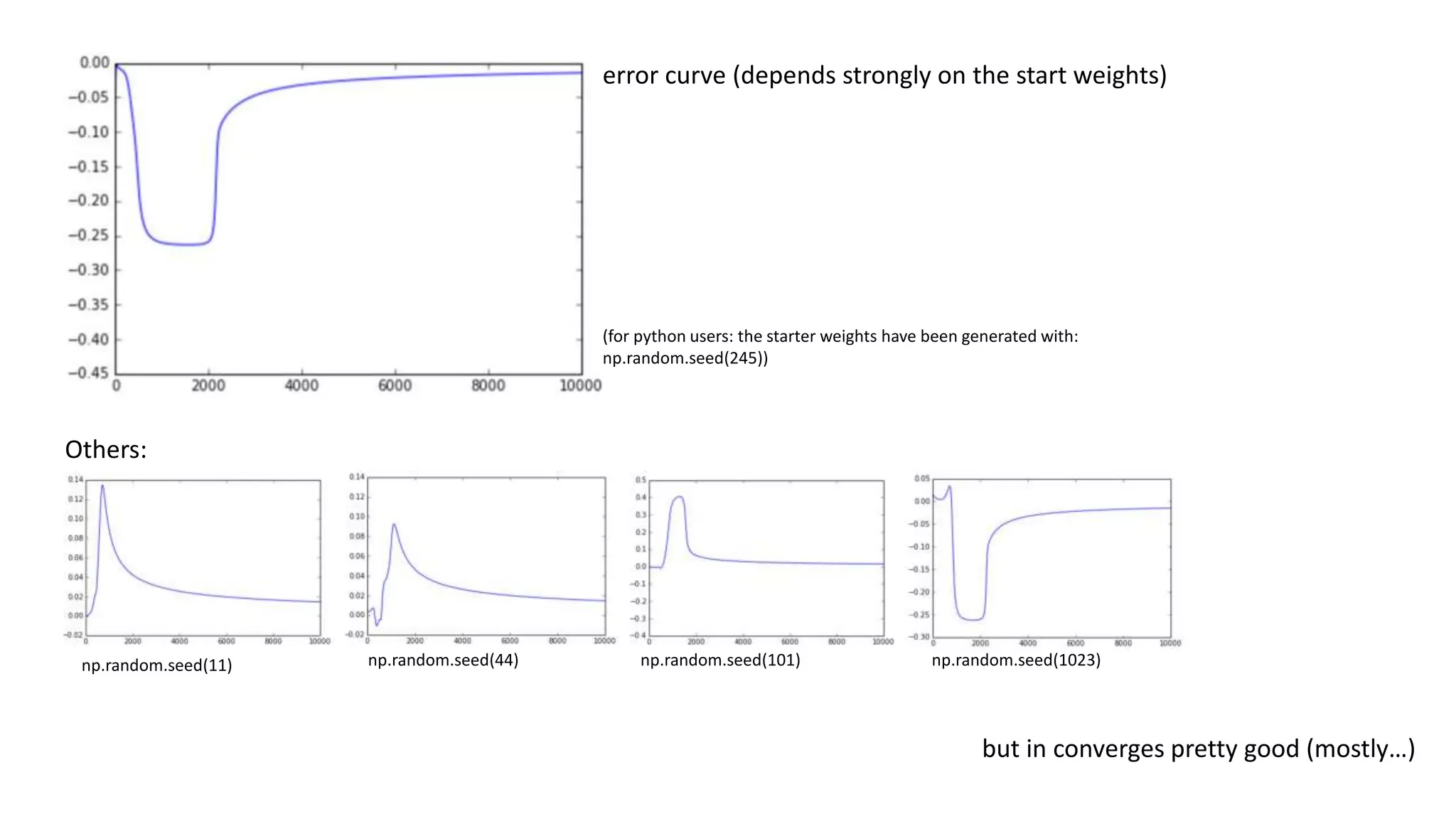
error curve (depends strongly on the start weights)
np.random.seed(11) np.random.seed(44) np.random.seed(101) np.random.seed(1023)
but in converges pretty good (mostly…)
Others:
(for python users: the starter weights have been generated with:
np.random.seed(245))
np.random.seed(25)
WOOPS!
Output:
0,0 -> [ 0.0214737 ]
0,1 -> [ 0.98097769]
1,0 -> [ 0.9810124 ]
1,1 -> [ 0.50051869] ? – probably runs into a local minimum…
That’s it so far – hope you had a good ride.
Obviously there are more questions coming up after this session, which I might dig into later:
• Why are there so different error curves?
• How to avoid a wrong output like the last error curve.
• How many iterations does a neural network has to do, to learn?
• How many neurons to take?
• How deep the layers should be (deep learning)?
• Are there other functions to use instead of the sigmoid function?
• Different nets working together
• etc etc…

Neural network - how does it work - I mean... literally!

  • 1.
    How does aneural network work … literally! I mean, … really literally! Don’t give me the formulas, Don’t give me the python code JUST GIVE ME THE NUMBERS! Ok, here it is ….
  • 2.
    NN HORIZON OR NO HORIZON Let’s startwith an easy neural network to classify images.
  • 3.
    NN HORIZON Every pixelvalue gets feed into the network
  • 4.
    HORIZON At Wikipedia youfind images like these, which show, that Every pixel value is feed into every neuron. Looks complicated! But the math is actually not that hard. It’ just a lot of calculations! So let’s break it down.
  • 5.
    HORIZON 1 0 Let’s focus onimages with two pixels only. (for now)
  • 6.
    HORIZON 1 0 And let’s breakit down to only one neuron! (for now)
  • 7.
    1 0 1 For every inputwe have a wanted outcome. here it is 1,0 -> 1 At first we do not know, what outcome the neural net will be calculating. ?
  • 8.
    1 0 1 * -0.16 * 0.99 RandomWeights To start with the calculations, we set some random weights for the different inputs. These can be any numbers, but mostly one starts in the range of -1 to 1. With these we calculate our first inputs to the neuron. ? = -0.16 = 0.00
  • 9.
    1 0 1 * -0.16 * 0.99 RandomWeights Then we add up the results for every weight. ? = -0.16 = 0.00 + -0.16
  • 10.
    1 * -0.16= -0.16 0 * 0.99 = 0.0 1 0 + -0.16 > 0,46 0 1 Then we do one “higher math” step (not really), and get out 0,46 (Actually we just put -0.16 as x into the sigmoid-function, which is explaind the next slide and might look complicated but really isn’t.) 0,46 rounds to 0 which which is wrong … (we wanted 1) But that’s all there is to get results from a neural network that’s all there is in a neuron!
  • 11.
    1 * -0.16= -0.16 0 * 0.99 = 0.0 1 0 + -0.16 > 0,46 0 1 Example Input: Output: -1000 0.0 -100 0.0 -10 0.00004 -5 0.0066 -1 0.2689 -0.75 0.3208 -0.25 0.4378 0.0 0.5 0.25 0.5621 0.75 0.6791 1 0.7310 5 0.9933 10 0.9999 100 1.0 1000 1.0 The “higher math”: With the sum of the weighted inputs (-0.16) -> we call the sigmoid-function(x) Whoohooo! But what it does, is actually pretty easy: It maps every input to a value between 0 and 1 (see examples left) When we put -0.16 into the function we get 0.46 as a result. If we round this value we get 0 as an outcome of our neuron. This is wrong! What to do? Change the weights!
  • 12.
    1 * -0.16= -0.16 0 * 0.99 = 0.0 1 0 + -0.16 > 0,46 0 0.546 * 1 = 0.546 0.546 * 0 = 0.0 * 1- 0,46 = 0,546 1 1 -0.16+-0.546 = 0.38 0.99 + 0.0 = 0,99 += += 0.16 -> 0.38 0.99 -> 0.99 New weights: To correct the weights, we… …calculate the output error (0.546) …calculate the error per weight and input …and add it to the old weight. That’s called “Backpropagation” (because it goes backwards)
  • 13.
    1 * 0.38= 0.38 0 * 0.99 = 0.0 + 0.38 > 0,59 1 1 0 AND THAT‘s IT! Well… basically it really is. It‘s all about getting input values to the right output values by adjusting the weights. But obviously neural nets have more than one neuron. And normally there is more than one input. Let‘s increase the input‘s first! Now we calculate again, and get the right output!
  • 14.
    1 1 0 1 0 1 Let‘s assume thereis another input [1,1] which we want to map to 0. Now we have: This has some influence on how we adjust the weights on the way back – have a look:
  • 15.
    1 * -0.16= -0.16 1 * -0.16 = -0.16 0 * 0.99 = 0.00 1 * 0.99 = 0.99 1 0 + -0.16 -> 0.460 0.83 -> 0.696 0 0.546 * 1 = 0.546 -0.696 * 1 = -0.696 0.546 * 0 = 0.0 -0.696 * 1 = -0.696 * 1- 0.460= 0.546 0- 0.696= -0.696 1 -0.16+ 0.546 -0.696 = -0.316 0.99+ 0.0 -0.696 = +0.293 += += 1 1 1 0 0 1 0.16 -> -0.316 0.99 -> +0.293 Round 1 Now it‘s 2 values to add here…: We do the same for both inputs All what changes is how we sum up the new weight
  • 16.
    -0.16 + (1* -0.546 + 1 * -0.696) = -0.16 + 0.546 - 0.696 = -0.316 We can write this update regarding to the errors in one line for each input weight: 0.99 + (0 * -0.546 + 1 * -0.696) = 0.99 + 0.000 - 0.696 = 0.293 0.16 -> -0.316 0.99 -> +0.293 0.546 * 1 = 0.546 -0.696 * 1 = -0.696 0.546 * 0 = 0.0 -0.696 * 1 = -0.696 * 1- 0.460= 0.546 0- 0.696= -0.696 -0.16+ 0.546 -0.696 = -0.316 0.99+ 0.0 -0.696 = +0.293 += += (we will do this again later when we have many weights…)
  • 17.
    1 * -0.316= -0.316 1 * -0.316 = -0.316 0 * 0.293 = 0.00 1 * 0.293 = 0.293 1 0 + -0.316 -> 0,421 -0.022 -> 0,494 0 0.578 * 1 = 0.578 -0.494 * 1 = -0.494 0,578 * 0 = 0.00 -0,494 * 1 = -0.494 * 1- 0,421= 0,578 0- 0,494= -0,494 1 -0.316+ 0.578 -0.494 = -0.232 0.293+ 0.0 -0.494 = -0.200 += += 1 1 0 0 0 1 -0.316 -> -0.232 +0.293 -> -0.200 Round 2 Still not right. So we do another round.
  • 18.
    1 * -0.232= 0.232 1 * -0.232 = 0.232 0 * -0.200 = 0.00 1 * -0.200 = -0.200 1 0 + -0.232 -> 0,442 -0.432 -> 0,393 01 1 0 -0.232 -> -0.067 -0.200 -> -0.594… … -> 1.087 … -> -0.934 … -> 0.483 … -> 0,340 … -> 0.277 … -> -1.238 … -> 0.527 … -> 0,304 … -> 0.568 … -> 0,276 … -> 0.431 … -> -1.515 … -> 0.968 … -> 0.021 … -> 3.426 … -> -7.271 Round 4 Round 3 Round 5 Round 6 Round 100 ……………………………………………………………………………………………………………………………. 1 0 And another And another And another … Till it fits!
  • 19.
    weight 1 (startedat -0.16) weight 2 (started at 0.99) sum of errors the error converges to 0.0 (hopefully :-)
  • 20.
    Ok, I letout oooone little thing, which we need later (with more neurons and more layers) We do not actually take the error-values directly to correct the weights, but a weighted error… Have a look at sig‘(x): The results are always between 0 and 1 If the NN is not sure if 1 or 0 is the right answer: max=0.5 > maps to 0.25 Sure if 1 or 0: min=0 or 1 > maps to ~ 0.0 multiply the error with simgoid derivate of the result: e.g.: result = 0.46, error = 1-0.46 = 0.54 sigmoid derivate of result : 0.248 value for correction: 0.546 * 0.248 = 0.134 This practice assures, we give those errors more importance where we are unsure about the answer. sig‘(x)= sig(x)*(1-sig(x)) sig(x)= 1 (1 + e )-x We used this to map results to 0 or 1: We use this to evaluate which errors are more important
  • 21.
    1 * -0.16= -0.16 0 * 0.99 = 0.0 1 0 + -0.16 > 0,46 0 0.134 * 1 = 0.134 0.134 * 0 = 0.0 * 1- 0,46 = 0.546 0.46 > 0.248 0.546 * 0.248 = 0.134 1 1 -0.16+ 0.134= -0.025 0.99 – 0.0 = -0,99 += += 0.16 -> -0.025 0.99 -> 0.99 Now the weights are corrected more cautious: 0.16 -> 0.38 0.99 -> 0.99 Corrected weights before: Basically only this number changes a bit
  • 22.
    1 * -0.16= -0.16 0 * 0.99 = 0.0 1 0 + -0.16 > 0,46 0 0.546 * 1 = 0.546 0.546 * 0 = 0.0 * 1- 0,46 = 0,546 1 1 -0.16+-0.546 = 0.38 0.99 + 0.0 = 0,99 += += 0.16 -> 0.38 0.99 -> 0.99 New weights: To correct the weights, we… …calculate the output error (0.546) …calculate the error per weight and input …and add it to the old weight. That’s called “Backpropagation” (because it goes backwards) (s. slide 12)
  • 23.
    This was fun– let’s try another more complicated example with our neuron …. XOR
  • 24.
    0 0 0 0 1 1 1 0 1 1 1 0 in out 0 00 0 1 1 1 0 1 1 1 0 XOR spoiler: does not work... (with one neuron)
  • 25.
    sum of error== 0! But…: [0,0] -> out = 0.5 -> error = -0.5 [0,1] -> out = 0.5 -> error = 0.5 [1,0] -> out = 0.5 -> error = 0.5 [1,1] -> out = 0.5 -> error = -0.5 The weights are actually both 0! If you think about it, it‘s pretty obvious. Every weight has to be the same, because a 1 or 0 leads to 0 or 1 in the same amount of cases For XOR to work we need more layers!
  • 26.
    0 1 1 ? We try itwith three input neurons and one output neuron Let’s look at only one input first.
  • 27.
    0 1 0.81 -0.84 0.299 0.90 -0.63 0.588 -0.77 0.88 0.707 -0.79 0.69 0.667 0.80 sig( 0*0.81+ 1*-0.84 ) = sig(-0.84) = 0.299 sig( 0.299*0.90 + 0.707*-0.63 + 0.667*0,80) = sig(-0.353) = 0.588 The forward calculation for one input The output is 1 that’s good! – let’s check the other inputs: layer0 layer1 In layer2 we have not 0 or 1 as input, but fractions! 1 !
  • 28.
    layer2layer0 layer1 0.81 -0.84 0.500 0.299 0.692 0.491 0.90 -0.63 0.630 0.588 0.662 0.619 -0.77 0.88 -0.79 0.69 0.80 0.500 0.707 0.315 0.527 0.500 0.667 0.310 0.474 first resultsfor all inputs (not so good…) The forward calculation for ALL FOUR inputs 1.0 1.0 1.0 1.0 For all 4 inputs the results are not so good… we have to update the weights… layer by layer…
  • 29.
    0.81 -0.84 0.84 -0.69-0.77 0.88 -0.79 0.69 0.75 l2_error 0-r1= -0.630 1-r2= 0.411 1-r3=0.337 0-r4= -0.619 l2_delta sig‘(0.63)*-0.63=-0.146 sig‘(0.58)* 0.41= 0.099 sig‘(0.66)* 0.34= 0.075 sig‘(0.62)*-0.62=-0.14 0.90 + (0.500*-0.146 + 0.299*0.099 + 0.692*0.075 + 0.491*-0.14) = 0.84 -0.63 + (0.500*-0.146 + 0.707*0.099 + 0.315*0.075 + 0.527*-0.14) = -0.69 0.80 + (0.500*-0.146 + 0.667*0.099 + 0.310*0.075 + 0.474*-0.14) = 0.75 same as before (but with more values…) 0.500 0.299 0.692 0.491 0.500 0.707 0.315 0.527 0.500 0.667 0.310 0.474 * * * * += += += += += += 0,0 -> r1= 0.630 0,1 -> r2= 0.588 1,0 -> r3= 0.662 1,1 -> r4= 0.619 Backward Propagation: Now we update the old weights regarding to the errors of all inputs. First in layer 2 0.90 -0.63 0.80
  • 30.
    0.795 -0.861 0.81 + (0*-0.033+ 0*0.018 + 1*0.014 + 1*-0.033) = 0.795 -0.84 + (0*-0.033 + 1*0.018 + 0*0.014 + 1*-0.033) = -0.861 Again as before (but with more values…) 0.500 0.299 0.692 0.491 * * * += += += += 0,0 -> r1= 0.5 0,1 -> r2= 0.299 1,0 -> r3= 0.692 1,1 -> r4= 0.491 l1_delta sig‘(0.500) *-0.132 =-0.033 sig‘(0.299) * 0.090 = 0.018 sig‘(0.692) * 0.068 = 0.014 sig‘(0.491) *-0.131 =-0.033 l1_error = l2_delta * weight of neuron 1 (to l2) 0,0 -> -0.146*0.90 = -0.132 0,1 -> 0.099*0.90 = 0.090 1,0 -> 0.075*0.90 = 0.068 1,1 -> 0.140*0.90 = -0.131 And now the weights in layer 1! The error in neuron1 is a fraction of the error in the output neuron (l2) Therefore we take the delta-error of layer2; neuron1 accounted 0.90 to this error: l2_delta * weight of neuron 1 to l2 And of this we get the delta again -> l1_delta * += += 0.81 -0.84 Neuron 1 in layer 1:
  • 31.
    error curve (dependsstrongly on the start weights) np.random.seed(11) np.random.seed(44) np.random.seed(101) np.random.seed(1023) but in converges pretty good (mostly…) Others: (for python users: the starter weights have been generated with: np.random.seed(245))
  • 32.
    np.random.seed(25) WOOPS! Output: 0,0 -> [0.0214737 ] 0,1 -> [ 0.98097769] 1,0 -> [ 0.9810124 ] 1,1 -> [ 0.50051869] ? – probably runs into a local minimum…
  • 33.
    That’s it sofar – hope you had a good ride. Obviously there are more questions coming up after this session, which I might dig into later: • Why are there so different error curves? • How to avoid a wrong output like the last error curve. • How many iterations does a neural network has to do, to learn? • How many neurons to take? • How deep the layers should be (deep learning)? • Are there other functions to use instead of the sigmoid function? • Different nets working together • etc etc…