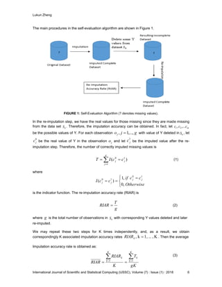
SlideShare a Scribd company logo
Lukun Zheng
International Journal of Scientific and Statistical Computing (IJSSC), Volume (7) : Issue (1) : 2018 1
A Two-Step Self-Evaluation Algorithm On Imputation
Approaches For Missing Categorical Data
Lukun Zheng lzheng@tntech.edu
Faculty of Department of Mathematics
Tennessee Technological University
Cookeville, TN 38501, United States of America
Abstract
Missing data are often encountered in data sets and a common problem for researchers in
different fields of research. There are many reasons why observations may have missing values.
For instance, some respondents may not report some of the items for some reason. The
existence of missing data brings difficulties to the conduct of statistical analyses, especially when
there is a large fraction of data which are missing. Many methods have been developed for
dealing with missing data, numeric or categorical. The performances of imputation methods on
missing data are key in choosing which imputation method to use. They are usually evaluated on
how the missing data method performs for inference about target parameters based on a
statistical model. One important parameter is the expected imputation accuracy rate, which,
however, relies heavily on the assumptions of missing data type and the imputation methods. For
instance, it may require that the missing data is missing completely at random. The goal of the
current study was to develop a two-step algorithm to evaluate the performances of imputation
methods for missing categorical data. The evaluation is based on the re-imputation accuracy rate
(RIAR) introduced in the current work. A simulation study based on real data is conducted to
demonstrate how the evaluation algorithm works.
Keywords: Categorical Variable, Imputation Methods, Missing Value, Re-Imputation Accuracy
Rate.
1. INTRODUCTION AND MOTIVATION
Data scientists are often faced with issues of missing data in different situations [1, 2]. There are
several reasons why observations may have missing values. For instance, one reason may be
that some respondents just do not report some of the variable for some reason. Researchers
have investigated the impact of missing data on statistical analyses [3]. The missing data may
lead to biased estimates and inflated standard errors. In addition, the power of statistical tests
may drop dramatically when there is a large amount of missing data in the data set.
Data often are missing in research in economics, sociology, and political science because
governments choose not to, or fail to, report critical statistics [4]. Sometimes missing values are
caused by the researcher. For example, when data collection is done improperly or mistakes are
made in data entry [5]. There are different types of missing data based on the underlying
formation process. Different forms of missing data have different impacts on the statistical
analyses. There are a lot of open resources about missing data and interested readers are
encouraged to refer to them for a more thorough discussion. Values in a data set are missing
completely at random (MCAR) if the events that lead to any data-item being missing are
independent both of observable variables and of unobservable parameters of interest, and occur
entirely at random [6]. When data are MCAR, the missing data are a random sample of the
observed data and the analysis performed on the data is unbiased. Missing at random (MAR)
occurs when the missingness is not random, but where missingness can be fully accounted for by
variables where there is complete information. For instance, males are less likely to enroll in a
depression survey than females but this has nothing to do with their level of depression. Finally,
Lukun Zheng
International Journal of Scientific and Statistical Computing (IJSSC), Volume (7) : Issue (1) : 2018 2
missing not at random (MNAR) (also known as nonignorable nonresponse) occurs when the
missingness is related to the value of the variable itself. To extend the previous example, this
would occur if men failed to enroll in a depression survey because of their level of depression. As
another example, respondents might be asked to indicate the number of times they are pulled
over due to speeding during the previous year. A missing response would be MNAR if individuals
who were pulled over for many times due to speeding during this period were more likely to leave
the item unanswered rather than report their behavior.
Given the potential problems caused by the presence of missing data, many methods have been
suggested for data imputation. People may refer to [7] for a comprehensive review of many of
these methods. Many missing data techniques have been suggested and developed. According
to [8], these missing data techniques can be roughly grouped into:
1. techniques ignoring incomplete observations,
2. imputation-based techniques,
3. weighting techniques, and
4. model-based techniques [2].
In this paper, we will ignore weighting techniques and mainly focus on the imputation-based
techniques and model-based techniques. The simple and widely used technique is the so-called
list wise deletion which ignore all incomplete observations and only focus on complete
observations. List wise deletion is easy to carry out and the result may be reliable and satisfactory
with small portion of observations with missing data. However, it fails if there is a large portion of
observations with missing data, which might be very common in high-dimensional case. In
addition, list wise deletion may lead to serious biases if the data are missing not at random.
Imputation-based techniques provide a way to replace missing values with suitable estimates,
which results in imputed complete data set. Many methods have been suggested for imputing
suitable responses to missing data. Among these techniques are mean or mode substitution,
regression imputation, k-nearest neighbor imputation, Hot Deck imputation, multiple imputation,
etc. In the imputation-based techniques, missing values are replaced by artificial values and it
may cause series biases. And this imputed data set in turn might lead to biased result in the
subsequent data analysis. And most of these imputation methods has been found inadequate in
reproducing known population parameters and standard errors [7].
Model-based imputation techniques performs parameter estimation. Two popular model-based
imputation techniques are regression-based and likelihood-based techniques [2, 9]. In regression-
based imputation, the missing values are imputed by a regression of the dependent variable with
missing values on the observed values of other independent variables for a given data set. In
likelihood-based imputation, the data are described based on a model and the parameters are
estimated by maximizing likelihood for a given data set [2].
The imputation methods can also be roughly classified into two: parametric imputation methods
and non-parametric imputation methods. The parametric imputation methods are usually superior
if the data set can be modeled adequately by a parametric model. For instance, the linear
regression can be used to conduct the imputation of missing quantitative values and logistic
regression can be used to conduct imputation of missing binary qualitative values [10, 11]. Non-
parametric imputation methods conduct imputation of missing data by capturing structures in the
data sets and they offer an alternative if the users have no idea of the actual distribution of the
data set. In other words, it is beneficial to use a non-parametric method in cases that the
relationship between the response and explanatory variables are unknown. For instance, the
nearest-neighbor (NN) imputation algorithm is one of the non-parametric methods used for
imputation of missing data in sample surveys [12]. Chen and Huang [13] constructed a genetic
system to impute in relational database systems. The machine learning methods also include
decision tree imputation, auto associative neural network and so forth.
Lukun Zheng
International Journal of Scientific and Statistical Computing (IJSSC), Volume (7) : Issue (1) : 2018 3
Once the imputation of missing data is done, it is crucial to evaluate the performance of the
imputation techniques used through determining the effect of imputation on subsequent statistical
inferences. All these imputation methods have pros and cons and they may perform well in one or
more situations but fails in others. And the comparison among these different imputation methods
have been studied in many situations. And these comparisons are mainly based on the potential
consequences in the subsequent data analysis caused by corresponding imputation methods.
For instance, [1] compares the performance of three imputation methods based on the estimation
accuracy of logistic regression parameters, standard errors and hypothesis testing results from
the imputed data using rounded multiple imputation for continuous data(MI), stochastic regression
imputation (SRI), and multiple imputation for categorical data, respectively. [14] studied the
performance of three missing value imputation techniques with respect to different rate of missing
values in the data set.
The purpose of this paper is to present a new self-evaluation algorithm of imputation approaches
for missing categorical data values. The new evaluation algorithm can be used to test a wide
range of imputation techniques of missing categorical data. The performance of several leading
imputation approaches is measured with respect to different rate of missing values in the data
set. To this end, the paper provides:
1. a description of several popular and modern imputation approaches, namely, MI, KNN,
C5.0 decision tree, Naive Bayes, and polytomous regression imputation- ordered (POLR).
2. a new self-evaluation algorithm for imputation approaches of missing categorical data.
3. a wide range of evaluation of quality of imputation with respect to the rate of missing data.
4. several simulation results based on real data.
The paper is organized as follows. Section 2 provides a description of the relevant imputation
approaches and our proposed self-evaluation algorithm. Section 3 explains details of the
experimental study and presents and analyzes the results. Finally, Section 4 summarizes the
paper.
2. IMPUTATION APPROACHES AND THE PROPOSED SELF-EVALUATION
ALGORITHM
In this section, we will introduce the imputation approaches used in this study and the proposed
self-evaluation algorithm.
2.1 Imputation Approaches
The imputation techniques used in this paper include mean imputation (MI), k nearest neighbor
imputation (KNN), C5.0 decision tree imputation, Naive Bayes (NB), and polytomous regression
imputation- ordered (POLR).
1. Mean Imputation (MI). In mean imputation, the missing values are imputed with the mean for
quantitative data or the most frequent value (mode) for qualitative data of the corresponding the
variable. Anderson et al [15] states that the sample mean provides an optimal estimate of the
most probable value in the case of normal distribution. The use of MI will shrink the sample
variance and affect the correlation between the imputed variable and other variables. Such
impact will be significant if there is a high percentage of missing values imputed using MI and the
subsequent statistical inferences might be misleading due to the too much centrally located
values created by MI [16].
2. K Nearest Neighbor Imputation (KNN). KNN is an efficient hot deck method to impute the
missing value, in which the missing values are imputed based on its k nearest neighbors in the
whole data set according to some metric. This method applies to both continuous variables or
discrete variables. For continuous variables, the most commonly used distance metric to
determine the k nearest neighbors is the Euclidean distance (Minkowski norm
Lukun Zheng
International Journal of Scientific and Statistical Computing (IJSSC), Volume (7) : Issue (1) : 2018 4
ppn
i
ii yxyxd
/1
1
),(








 

with p = 2). Then the missing values is imputed as the average or
weighted average of these k nearest neighbors. For discrete variables, such as texts, other types
of distance metric such as Hamming distance or overlap metric can be used to determine the k
nearest neighbors. Then the missing value is imputed as the most frequent value among the k
nearest neighbors. Usually k is taken as a small positive integer. When k = 1, the KNN method is
the similar response pattern imputation (SRPI), which consists of identifying the nearest neighbor
(the most similar observation) and imputing the missing value by copying the value of this nearest
neighbor. An advantage over mean imputation is that the replacement values are influenced only
by the most similar cases rather than by all cases. Several studies have found that the k-NN
method performs well or better than other methods in certain contexts [17, 18]. A shortcoming of
the KNN imputation is that it is sensitive to the local structure of the data.
3. C5.0 Decision Tree Imputation (C5.0) [19]. C5.0 extends the C4.5 classification algorithms
described in [20]. It is a well-known machine learning algorithm which has a good internal method
to treat missing values. Hurley (2017) did a comparative study, with other simple methods to treat
missing values, and concluded that it was one of the best methods. C5.0 uses the information
gain ratio measure to choose a good test on one categorical variable that has mutually exclusive
outcomes rOOO ,...,, 21 for a given training data set T. Then T is partitioned into rTTT ,...,, 21
with iT consisting of the observations in T that will be classified as iO by the test. The same
algorithm is then applied to each subset iT until a stop criterion is encountered. When an instance
in T with known value is assigned to a subset iT , this indicates that the probability of that
instance belonging to subset iT is 1 and to all other subsets is 0. When the value is missing,
C5.0 associates to each instance in iT a weight representing the probability of that instance
belonging to iT . This probability is estimated as the sum of the weights of instances in T known
to satisfy the test with outcome iO , divided by the sum of weights of the cases in T with known
values on the variable.
4. Naive-Bayes (NB). Naive Bayes is an also a machine learning technique [21]. The algorithm
works with discrete data and requires only one pass through the database to generate a
classification model, which makes it computationally efficient. This algorithm assumes that the
feature or attribute values are conditionally independent given the class of the attribute,


d
i id cxPcxxxP 121 )|()|,...,,( , where ix is the ith attribute, c represents the class, and d
is the number of attributes. The data are divided into two parts: 1) training database that includes
all records for which class attribute is complete and 2) testing database for which the records are
missing. Imputation based on the Naive Bayes consists of two simple steps. First, the conditional
probabilities )|( cxP i and the prior probabilities )(cP are estimated based on the training
database. Then the estimated probabilities are then used to conduct imputation of the missing
values of the attributes in testing database based on the rule:
.)|().(maxarg),...,,|(maxarg 121 

d
i icdc cxPcPxxxcP
5. Polytomous Regression Imputation- Ordered (POLR). This is a regression imputation
method based on proportional odds model. The proportional odds model is estimated first based
on available complete or incomplete observations and then used to impute missing values of a
variable based on the fitted values from the model.
Lukun Zheng
International Journal of Scientific and Statistical Computing (IJSSC), Volume (7) : Issue (1) : 2018 5
Imputation Approaches Works with continuous
data?
Works with discrete data?
MI Yes Yes
KNN Yes Yes
C5.0 No Yes
Naïve-Bayes No Yes
POLR Yes Yes
TABLE 1: Summary of Imputation Approaches.
Table 1 summarized the imputation approaches used in this study.
2.2 The Self-Evaluation Algorithm
The evaluation algorithm proposed in the paper consists of two steps: imputation and re-
imputation. Given a data set, let Y be a categorical variable with missing values in the data set
and let T
dXXXX ),...,,( 21 corresponds all other variables. Assume that there are n
observations );,...,,( 21 idi yxxxo  , ni ,...,2,1 in the data set. We may assume that there are
no missing values for other variables in the data set. Split the data set into two sets: one set 0S
with observations with no missing values and the other set 1S of observations with missing
values. Assume that there are 0n observations in 0S and 1n observations in 1S . Therefore, 1n is
the number of missing values in the data set. And
n
n
r 1
 is the proportion of missing values in
Y . We select one imputation technique to fill in the missing value. To evaluate the performance
of the selected imputation technique, we propose the following self-evaluation algorithm.
Step 1 (Imputation): Conduct the imputation of missing values in 1S using the selected imputation
technique to obtain an imputed complete data set.
Step 2 (Re-imputation): From the imputed complete data set, delete certain number g of values
of Y from the data set 0S S0 using appropriate method to obtain a new incomplete data set. Then
re-impute the missing values using the same imputation method in Step 1. Here the method to
deleted values of Y must be chosen to keep the type of missing values the same as those in the
original data set. For instance, if the missing value in the original data set is missing completely at
random, then we must delete the values of Y in S0 completely at random.
Lukun Zheng
International Journal of Scientific and Statistical Computing (IJSSC), Volume (7) : Issue (1) : 2018 6
The main procedures in the self-evaluation algorithm are shown in Figure 1.
FIGURE 1: Self-Evaluation Algorithm (? denotes missing values).
In the re-imputation step, we have the real values for those missing since they are made missing
from the data set 0S . Therefore, the imputation accuracy can be obtained. In fact, let mccc ,..., 21
be the possible values of Y. For each observation gjoj ,...,1,  with value of Y deleted in 0S , let
0
jc be the real value of Y in the observation jo and let
1
jc be the imputed value after the re-
imputation step. Therefore, the number of correctly imputed missing values is
(1)
where
is the indicator function. The re-imputation accuracy rate (RIAR) is
(2)
where g is the total number of observations in 0S with corresponding Y values deleted and later
re-imputed.
We may repeat these two steps for K times independently, and, as a result, we obtain
correspondingly K associated imputation accuracy rates K,...1,k, kRIAR . Then the average
Imputation accuracy rate is obtained as:
(3)


g
j
jj ccIT
1
10
)(


 

Otherwise
ccif
ccI jj
jj
,0
,1
)(
10
10
g
T
RIAR 
gK
T
K
RIAR
RIAR
K
k
k
K
k
k  
 11
Lukun Zheng
International Journal of Scientific and Statistical Computing (IJSSC), Volume (7) : Issue (1) : 2018 7
where kT is the number of correctly imputed missing values in the kth repetition.
2.3 Estimation and Comparison
Due to the law of large numbers, the average imputation accuracy rate tends to be the expected
imputation accuracy rate under certain assumptions. In other words, as we do sufficient number K
of repetitions of the algorithm, the average re-imputation accuracy rate will approach the true re-
imputation accuracy rate and can, therefore, can be used to measure the performance of the
imputation technique.
Theorem 1. Given a data set with missing categorical values and an imputation technique, let
RIAR be the average re-imputation accuracy rate, then it converges to the expected re-
imputation accuracy rate )(RIARE in probability. That is,
(4)
The following theorem is a direct result from central limit theorem on proportions.
Theorem 2. Given a data set with missing categorical values and an imputation technique, let
RIAR be the average re-imputation accuracy rate, then
(5)
Where ./)](1)[( KRIARERIARERIAR

From Theorems 1, 2, and Slutsky's theorem, we have the following corollary.
Corollary 1. Given a data set with missing categorical values and an imputation technique, let
RIAR be the average re-imputation accuracy rate, then
(6)
These theorems and corollary provide statistical tools for estimation and comparison of the re-
imputation accuracy rates based on different imputation approaches on a data set with missing
categorical data.
The expected imputation accuracy rate E(IAR) is an important measure of the performance of a
given imputation technique. However, there are many cases in practice that no real values of the
missing value are known, which makes it impossible to obtain the imputation accuracy rate. In the
re-imputation step of the proposed algorithm, it becomes possible to obtain the re-imputation
accuracy rate since the missing values of Y are made missing in the data set 0S and we do have
the corresponding real values. The re-imputation accuracy rate can be obtained to measure the
performance of the imputation technique. The fact that the same imputation technique is used to
evaluate the performance of itself leads to the name of the proposed “self-evaluation algorithm for
imputation approaches". The proposed algorithm is applicable to a wide range of imputation
methods. There are several evaluation algorithms which have been proved to be effective in
many situations for comparing different imputation methods [1, 8]. However, they usually assume
strong assumptions on the type of variables and statistical models. Our algorithm is based on the
.Kas),(  RIARERIAR P
.Kas,1)N(0,
)(

 L
RIAR
RIARERIAR

.Kas,1)N(0,
/)1(
)(


 L
KRIARRIAR
RIARERIAR
Lukun Zheng
International Journal of Scientific and Statistical Computing (IJSSC), Volume (7) : Issue (1) : 2018 8
expected re-imputation accuracy rate, which assumes no assumptions on the missing values in
the dataset and models on evaluations. Hence, it is valid to perform evaluations on a wide range
of imputation methods in different situations. In addition, the proposed algorithm is easier to
perform evaluations compared with many other algorithms. Imputation methods are usually
evaluated on how they perform for inference about target parameters based on a statistical model
such as a regression model. Sometimes, these statistical models are complicated and come with
strong assumptions, which makes the evaluations hard to perform and restrict the applications to
some limited situations. In our proposed algorithm, the performance can be easily obtained in a
two-step procedure based on a simple valuation measure E(RIAR) and very basic assumptions.
In the next section, we will use the proposed evaluation algorithm to measure the performance of
the five imputation approaches mentioned in section 2.1 based on a real data set.
3. EXPERIMENT AND RESULTS
The main purpose of the experiments is to empirically evaluate the performances of imputation
approaches based on their re-imputation accuracy rates using the proposed self-evaluation
algorithm. We will start with the description of the data sets. The experimental results and
analysis will follow.
Variables Categories Frequency Relative Frequency
Rank (Ordinal) 1. Assistant Professor 67 0.298
2. Associate Professor 64 0.284
3. Full Professor 94 0.418
Missing 0 NA
Discipline
(Nominal)
1. Theoretical (A) 95 0.422
2. Applied (B) 130 0.578
Missing 0 NA
yrs.service
(Ordinal)
1. Less than 6 71 0.338
2. From 6 to 15 62 0.295
3. More than 15 77 0.367
Missing 15 NA
Salary
(Ordinal)
1. Less than $85,000 62 0.305
2. From $85,000 to
$110,000
76 0.374
3. More than $110,000 65 0.321
Missing 22 NA
TABLE 2: Descriptive Summary of Variables In The Data Set.
3.1 Estimation and Comparison
The experiments are based on the data set “Salaries" included in the R package “car” [22]. The
data set included the 2008-09 nine-month academic salaries for assistant professors, associate
professors and full professors in a college in the U.S. After some initial data processing, the
resulting data set contained information of 67 assistant professors, 64 associate professors, and
94 full professors on four variables, namely, rank, discipline, years of service (yrs.service), and
salary. The variable “rank” has three different levels: assistant professor (AsstProf), associate
professor (AssocProf), and full professor (Prof). The variable “discipline” has two levels:
theoretical department (A) and applied department (B). The variable “years of service”
(yrs.service) is classified into three categories with level 1 if it is less than six years, level 2 if it is
from six years to fifteen years, and level 3 if it is more than fifteen years. Similarly, the variable
“salary” is also classified into three categories with level 1 if it is less than $ 85,000, level 2 if it is
more than or equal to $ 85,000 and less than $110,000, and level 3 if it is more than $ 110,000.
There are fifteen missing values for the variable “years of service” (yrs.service) and twenty two
Lukun Zheng
International Journal of Scientific and Statistical Computing (IJSSC), Volume (7) : Issue (1) : 2018 9
missing values for the variable “salary”. A descriptive summary of the resulting data set is given in
table 2.
3.2 Experimental Setup
The experiments were performed in the following procedure. The data set was first imputed using
a selected imputation method. Next, the missing data were generated randomly, using the MCAR
mechanism, from the data set S0(the set containing complete observations) in the following
amounts: 5%, 10%, 20%, and 30%. Then the missing data were again imputed using the same
imputation method and the re-imputation accuracy rate (RIAR) of the selected imputation method
was calculated and evaluated through estimation. The imputation methods used includes mean
imputation (MI), KNN, C5.0 decision tree imputation, Naive-Bayes(NB), and polytomous
regression imputation-ordered (POLR). The results of the above experiments were then
examined and compared.
3.3 Experimental Results
The experiments report the re-imputation accuracy rate against four amounts of missing values,
for five different imputation methods mentioned above. For KNN, three neighbors are considered.
In these experiment, the accuracy rate is measured based on a zero-one loss, which is commonly
used to evaluate the performance of imputation methods. We assume a uniform cost for all the
categories of all variables. A future study would consider different categories having different
associated costs.
Table 3 presents the average re-imputation accuracy rate of these five different imputation
methods at different amounts of missing values based on K = 1000 repetitions. The best results
based on these average RIAR's are highlighted in bold. We note that the highest re-imputation
accuracy rate over all amounts of missing data is 71.9% for 5% missing data re-imputed by the
C50 decision tree imputation for the variable yrs.service. The highest re-imputation accuracy rate
over all amounts of missing data is 80.6% for 10% missing data re-imputed by the C50 decision
tree imputation for the variable salary. Based on these results, we notice that C50 is in general
the best imputation method among these five imputation methods for the missing values in the
data set.
Variable
Missing
(%)
Imputation Methods
MI KNN C50 Naïve Bayes POLR
yrs.service
5 0.370 0.633 0.719 0.667 0.699
10 0.369 0.607 0.715 0.675 0.694
20 0.375 0.576 0.714 0.674 0.697
30 0.372 0.545 0.714 0.676 0.693
salary
5 0.408 0.635 0.805 0.797 0.583
10 0.404 0.608 0.806 0.801 0.585
20 0.403 0.565 0.802 0.802 0.584
30 0.403 0.529 0.799 0.799 0.590
TABLE 3: Average re-imputation accuracy rates for two variables, five imputation methods and four
amounts of missing data based on 1000 repetitions (Best average RIAR's are shown in bold).
3.4 Statistical Comparison
Now we use test of significance to compare the performance of the imputation methods based on
the results of re-imputation accuracy rates. We analyze the statistical significance of differences
in re-imputation accuracy rates between imputation methods at 95% level of significance.
We want to test whether two mean re-imputation accuracy rates between two different imputation
methods for a given amount of missing data are different. The null hypothesis H0 is that they are
the same. Since the average re-imputation accuracy rates are computed based on K = 1000
Lukun Zheng
International Journal of Scientific and Statistical Computing (IJSSC), Volume (7) : Issue (1) : 2018 10
independent repetitions, a Z-test is applied for the comparison. The standard error of the
sampling distribution of the accuracy rate difference is
,
where
is the pooled sample accuracy rate ( Knn  21 ). Here 1
ˆp and 2
ˆp denotes the sample re-
imputation accuracy rates of two selected imputation methods, respectively.
For illustration, we test the significance of differences in re-imputation accuracy rates using KNN
and all other methods at different amounts of missing data. The results are summarized in table 4.
Variable
Missing
(%)
Imputation Methods
MI
Significance
(z-score)
C50
Significance
(z-score)
Naïve
Bayes
Significance
(z-score)
POLR
Significance
(z-score)
yrs.service
5 (-11.77) + + (4.12) (1.59) + + (3.14)
10 (-10:65) + + (5:11) + + (3:18) + + (4:08)
20 (-9:01) + + (6:46) + + (4:55) + + (5:63)
30 (-7:78) + + (7:82) + + (6:01) + + (6:83)
salary
5 (-10:14) + + (8:44) + + (8:01) (-2:39)
10 (-9.13) + + (9:73) + + (9:45) (-1:03)
20 (-7:23) + + (11:38) + + (11:39) (0:87)
30 (-5:63) + + (12:77) + + (12:78) + + (2:74)
TABLE 4: Statistical significance of the difference of re-imputation accuracy rates using KNN and other
methods at different amounts of missing data. Here, “++" indicates that the given imputation method
(columns) gives statistically significantly better re-imputation accuracy rate than KNN; “ " indicates that
the given imputation method (columns) gives statistically significantly worse re-imputation accuracy rate than
KNN; “ " indicates that the difference between the accuracy rates using the given imputation methods and
KNN is insignificant.
4. CONCLUSION
In this paper, we have introduced a new evaluation algorithm for imputation methods of missing
categorical values. There are two main steps in the algorithm. In the first step, the incomplete
data set is imputed using a selected imputation method to obtain an imputed complete data set
first. In the second step, a certain amount of missing values are generated from the originally
existing observations in the imputed complete data set and then these missing values get re-
imputed. The re-imputation accuracy rate is obtained based on certain number of repetitions of
this process and used to evaluate the performance of selected imputation method.
From Table 3 and 4, we can see that, among the selected imputation methods, C50
reconstructed the missing data in a better manner in general. The Naïve Bayes methods was
comparable to C50 only for the variable “salary” when the amount of missing values is 20 percent
or 30 percent. The mean imputation method produced worse results compared to other methods.
K
pp
nn
ppSE
)1(211
)1(
21








2
ˆˆˆˆ 21
21
2211 pp
nn
pnpn
p





Lukun Zheng
International Journal of Scientific and Statistical Computing (IJSSC), Volume (7) : Issue (1) : 2018 11
The algorithm assumes no assumptions on the missing values. That is, it applied to any type of
missing data (MCAR, MAR, or missing not at random). In addition, researchers can evaluate
most of imputation methods available for categorical data using our algorithm on a specific given
data set. The aim of the algorithm is to two-fold. First, it introduces an evaluation algorithm of
imputation methods for categorical data in a data set and, therefore, provides “the best"
imputation method for the missing categorical data. Second, it can shed some insights on the
“true reason” of missing values in the data set based on the performance of different imputation
methods.
In this paper, we only studied the evaluation algorithm for missing categorical data. The
evaluation algorithm for missing continuous data needs to be studied in future works.
5. REFERENCES
[1] W.H. Finch. “Imputation methods for missing categorical questionnaire data: a comparison
of approaches.” Journal of Data Science, vol. 8, pp. 361-378, 2010.
[2] R.J.A. Little. and D.B. Rubin. Statistical Analysis with Missing Data. New York: Wiley, 1987.
[3] E. D. de Leeuw, J. Hox, and M. Husman. “Prevention and treatment of item nonresponse.”
Journal of Official Statistics, vol. 19, pp. 277-314, 2003.
[4] S. F. Messner. “Exploring the Consequences of Erratic Data Reporting for Cross- National
Research on Homicide.” Journal of Quantitative Criminology, vol. 8, pp.155-173, 1992.
[5] D. J. Hand, H. J. Adér, and G. J. Mellenbergh. “Advising on Research Methods: A
Consultant's Companion.” Huizen, Netherlands: Johannes van Kessel. pp. 305-332, 2008.
[6] J. L. Schafer. Analysis of Incomplete Multivariate Data. Chapman and Hall, 1997.
[7] J. L. Schafer and J. W. Graham. “Missing data: Our view of the state of the art.”
Psychological Methods, vol. 7, pp.147-177, 2002.
[8] I. Myrtverit and E. Stensrud. “Analyzing data sets with missing data: an empirical evaluation
of imputation methods and likelihood-based methods.” IEEE Transactions On Software
Engineering, vol. 27, pp.999-1013, 2001.
[9] D.B. Rubin. “Multiple imputation after 18+ years.” J. Am. Stat. Assoc, vol. 91, pp. 473-489,
1996.
[10] S.C. Zhang, et al. “Optimized parameters for missing data imputation.” PRICAI, vol. 6, pp.
1010-1016, 2006.
[11] Q. Wang and J. Rao, “Empirical likelihood-based inferences in linear models with missing
data.” Scand. J. Statist, vol. 29, pp. 563-576, 2002.
[12] J. Chen and J. Shao. “Jackknife variance estimation for nearest-neighbor imputation.” J.
Amer. Statist, Assoc, vol. 96, pp. 260-269, 2001.
[13] S.M. Chen and C.M. Huang. “Generating weighted fuzzy rules from relational database
systems for estimating null values using genetic algorithms.” IEEE Transactions on Fuzzy
Systems, vol. 11, pp. 495-506, 2003.
[14] R.S. Somasundaram and R. Nedunchezhian. “Evaluation of three simple imputation
methods for enhancing preprocessing of data with missing values.” International Journal of
Computer Applications, vol. 21, pp. 14-19, 2011.
Lukun Zheng
International Journal of Scientific and Statistical Computing (IJSSC), Volume (7) : Issue (1) : 2018 12
[15] A.B. Anderson, A. Basilevsky, and D.P.J. Hum. “Missing data: a review of the literature,” in
Handbook of Survey Research. New York: Academic Press, 1983, pp. 415-492.
[16] M.J. Rovine and M. Delaney. ” Missing data estimation in developmental research,” in
Statistical Methods in Longitudinal Research: Principles and Structuring Change, A. Von
Eye ed. 1, New York: Academic Press, pp. 35-79.
[17] O. Troyanskaya, M. Cantor, and G. Sherlock. “Missing value estimation methods for DNA
microarrays.” Bioinformatics, vol. 17, pp. 520-525, 2001.
[18] J. Chen and J. Shao. “Nearest neighbor imputation for survey data.” Journal of Official
Statistics, vol. 16, pp. 113-131, 2000.
[19] L. Hurley. “Missing covariates in causal inference matching: Statistical imputation using
machine learning and evolutionary search algorithms.” Doctoral dissertation, Fordham
University, 2017.
[20] J. R. Quinlan. C4.5: Programs for machine learning, Morgan Kaufman, Los Altos, CA, 1993.
[21] R.O. Duda and P.E. Hart. Pattern Classification and Scene Analysis, New York: Wiley,
1973.
[22] J. Fox, S. Weisberg, D. Adler, D. Bates, G. Baud-Bovy, S. Ellison, ... and R. Heiberger.
Package “car”, Companion to Applied Regression. R Package version, 2-1, 2016.

More Related Content

What's hot

Statistical analysis and interpretation
Statistical analysis and interpretationStatistical analysis and interpretation
Statistical analysis and interpretation
Dave Marcial
 
Imputation techniques for missing data in clinical trials
Imputation techniques for missing data in clinical trialsImputation techniques for missing data in clinical trials
Imputation techniques for missing data in clinical trials
Nitin George
 
Data Analysis and Statistics
Data Analysis and StatisticsData Analysis and Statistics
Data Analysis and Statistics
T.S. Lim
 
Unit 4 editing and coding (2)
Unit 4 editing and coding (2)Unit 4 editing and coding (2)
Unit 4 editing and coding (2)
kalailakshmi
 
Concept of Inferential statistics
Concept of Inferential statisticsConcept of Inferential statistics
Concept of Inferential statistics
Sarfraz Ahmad
 
Data Analysis
Data AnalysisData Analysis
Data Analysis
sikander kushwaha
 
A review of statistics
A review of statisticsA review of statistics
A review of statistics
edisonre
 
Edisons Statistics
Edisons StatisticsEdisons Statistics
Edisons Statisticsteresa_soto
 
Imputation of missing data in clinical trials
Imputation of missing data in clinical trialsImputation of missing data in clinical trials
Imputation of missing data in clinical trials
Seema Ahirwar
 
Spss introductory session data entry and descriptive stats
Spss introductory session data entry and descriptive statsSpss introductory session data entry and descriptive stats
Spss introductory session data entry and descriptive stats
e1033930
 
Basic Statistics & Data Analysis
Basic Statistics & Data AnalysisBasic Statistics & Data Analysis
Basic Statistics & Data Analysis
Ajendra Sharma
 
Analytical Chemistry and Statistics in Exposure Science
Analytical Chemistry and Statistics in Exposure ScienceAnalytical Chemistry and Statistics in Exposure Science
Analytical Chemistry and Statistics in Exposure ScienceLarry Michael
 
notes on correlational research
notes on correlational researchnotes on correlational research
notes on correlational researchSiti Ishark
 
SheffieldR July Meeting - Multiple Imputation with Chained Equations (MICE) p...
SheffieldR July Meeting - Multiple Imputation with Chained Equations (MICE) p...SheffieldR July Meeting - Multiple Imputation with Chained Equations (MICE) p...
SheffieldR July Meeting - Multiple Imputation with Chained Equations (MICE) p...
Paul Richards
 
Basic Concepts of Inferential statistics
Basic Concepts of Inferential statisticsBasic Concepts of Inferential statistics
Basic Concepts of Inferential statistics
Statistics Consultation
 
SOC2002 Lecture 11
SOC2002 Lecture 11SOC2002 Lecture 11
SOC2002 Lecture 11Bonnie Green
 

What's hot (18)

Statistical analysis and interpretation
Statistical analysis and interpretationStatistical analysis and interpretation
Statistical analysis and interpretation
 
Imputation techniques for missing data in clinical trials
Imputation techniques for missing data in clinical trialsImputation techniques for missing data in clinical trials
Imputation techniques for missing data in clinical trials
 
Data Analysis and Statistics
Data Analysis and StatisticsData Analysis and Statistics
Data Analysis and Statistics
 
Unit 4 editing and coding (2)
Unit 4 editing and coding (2)Unit 4 editing and coding (2)
Unit 4 editing and coding (2)
 
Concept of Inferential statistics
Concept of Inferential statisticsConcept of Inferential statistics
Concept of Inferential statistics
 
Data analysis
Data analysisData analysis
Data analysis
 
Data Analysis
Data AnalysisData Analysis
Data Analysis
 
A review of statistics
A review of statisticsA review of statistics
A review of statistics
 
Edisons Statistics
Edisons StatisticsEdisons Statistics
Edisons Statistics
 
Imputation of missing data in clinical trials
Imputation of missing data in clinical trialsImputation of missing data in clinical trials
Imputation of missing data in clinical trials
 
Spss introductory session data entry and descriptive stats
Spss introductory session data entry and descriptive statsSpss introductory session data entry and descriptive stats
Spss introductory session data entry and descriptive stats
 
Basic Statistics & Data Analysis
Basic Statistics & Data AnalysisBasic Statistics & Data Analysis
Basic Statistics & Data Analysis
 
Analytical Chemistry and Statistics in Exposure Science
Analytical Chemistry and Statistics in Exposure ScienceAnalytical Chemistry and Statistics in Exposure Science
Analytical Chemistry and Statistics in Exposure Science
 
Final Project
Final ProjectFinal Project
Final Project
 
notes on correlational research
notes on correlational researchnotes on correlational research
notes on correlational research
 
SheffieldR July Meeting - Multiple Imputation with Chained Equations (MICE) p...
SheffieldR July Meeting - Multiple Imputation with Chained Equations (MICE) p...SheffieldR July Meeting - Multiple Imputation with Chained Equations (MICE) p...
SheffieldR July Meeting - Multiple Imputation with Chained Equations (MICE) p...
 
Basic Concepts of Inferential statistics
Basic Concepts of Inferential statisticsBasic Concepts of Inferential statistics
Basic Concepts of Inferential statistics
 
SOC2002 Lecture 11
SOC2002 Lecture 11SOC2002 Lecture 11
SOC2002 Lecture 11
 

Similar to A Two-Step Self-Evaluation Algorithm On Imputation Approaches For Missing Categorical Data

Twala2007.doc
Twala2007.docTwala2007.doc
Twala2007.docbutest
 
Zuur et al 2010 methods in ecology and evolution a protocol for data explorat...
Zuur et al 2010 methods in ecology and evolution a protocol for data explorat...Zuur et al 2010 methods in ecology and evolution a protocol for data explorat...
Zuur et al 2010 methods in ecology and evolution a protocol for data explorat...Lisiane Zanella
 
SPSS GuideAssessing Normality, Handling Missing Data, and Calculating Scores...
SPSS GuideAssessing Normality, Handling Missing Data, and Calculating  Scores...SPSS GuideAssessing Normality, Handling Missing Data, and Calculating  Scores...
SPSS GuideAssessing Normality, Handling Missing Data, and Calculating Scores...
ahmedragab433449
 
Classification Scoring for Cleaning Inconsistent Survey Data
Classification Scoring for Cleaning Inconsistent Survey DataClassification Scoring for Cleaning Inconsistent Survey Data
Classification Scoring for Cleaning Inconsistent Survey Data
CSCJournals
 
Classification Scoring for Cleaning Inconsistent Survey Data
Classification Scoring for Cleaning Inconsistent Survey DataClassification Scoring for Cleaning Inconsistent Survey Data
Classification Scoring for Cleaning Inconsistent Survey Data
CSCJournals
 
Machine Learning Approaches and its Challenges
Machine Learning Approaches and its ChallengesMachine Learning Approaches and its Challenges
Machine Learning Approaches and its Challenges
ijcnes
 
Data science notes for ASDS calicut 2.pptx
Data science notes for ASDS calicut 2.pptxData science notes for ASDS calicut 2.pptx
Data science notes for ASDS calicut 2.pptx
swapnaraghav
 
IT-601 Lecture Notes-UNIT-2.pdf Data Analysis
IT-601 Lecture Notes-UNIT-2.pdf Data AnalysisIT-601 Lecture Notes-UNIT-2.pdf Data Analysis
IT-601 Lecture Notes-UNIT-2.pdf Data Analysis
Dr. Radhey Shyam
 
A Magnified Application of Deficient Data Using Bolzano Classifier
A Magnified Application of Deficient Data Using Bolzano ClassifierA Magnified Application of Deficient Data Using Bolzano Classifier
A Magnified Application of Deficient Data Using Bolzano Classifier
journal ijrtem
 
Unit 8 data analysis and interpretation
Unit 8 data analysis and interpretationUnit 8 data analysis and interpretation
Unit 8 data analysis and interpretation
Asima shahzadi
 
Statistical Approaches to Missing Data
Statistical Approaches to Missing DataStatistical Approaches to Missing Data
Statistical Approaches to Missing Data
DataCards
 
Assigning Scores For Ordered Categorical Responses
Assigning Scores For Ordered Categorical ResponsesAssigning Scores For Ordered Categorical Responses
Assigning Scores For Ordered Categorical Responses
Mary Montoya
 
TECHNICAL REVIEW: PERFORMANCE OF EXISTING IMPUTATION METHODS FOR MISSING DATA...
TECHNICAL REVIEW: PERFORMANCE OF EXISTING IMPUTATION METHODS FOR MISSING DATA...TECHNICAL REVIEW: PERFORMANCE OF EXISTING IMPUTATION METHODS FOR MISSING DATA...
TECHNICAL REVIEW: PERFORMANCE OF EXISTING IMPUTATION METHODS FOR MISSING DATA...
IJDKP
 
TECHNICAL REVIEW: PERFORMANCE OF EXISTING IMPUTATION METHODS FOR MISSING DATA...
TECHNICAL REVIEW: PERFORMANCE OF EXISTING IMPUTATION METHODS FOR MISSING DATA...TECHNICAL REVIEW: PERFORMANCE OF EXISTING IMPUTATION METHODS FOR MISSING DATA...
TECHNICAL REVIEW: PERFORMANCE OF EXISTING IMPUTATION METHODS FOR MISSING DATA...
IJDKP
 
Research and Statistics Report- Estonio, Ryan.pptx
Research  and Statistics Report- Estonio, Ryan.pptxResearch  and Statistics Report- Estonio, Ryan.pptx
Research and Statistics Report- Estonio, Ryan.pptx
RyanEstonio
 
A Framework for Statistical Simulation of Physiological Responses (SSPR).
A Framework for Statistical Simulation of Physiological Responses (SSPR).A Framework for Statistical Simulation of Physiological Responses (SSPR).
A Framework for Statistical Simulation of Physiological Responses (SSPR).
Waqas Tariq
 
Stat11t chapter1
Stat11t chapter1Stat11t chapter1
Stat11t chapter1
raylenepotter
 
Stat11t Chapter1
Stat11t Chapter1Stat11t Chapter1
Stat11t Chapter1gueste87a4f
 
Journal for Clinical Studies: Close Cooperation Between Data Management and B...
Journal for Clinical Studies: Close Cooperation Between Data Management and B...Journal for Clinical Studies: Close Cooperation Between Data Management and B...
Journal for Clinical Studies: Close Cooperation Between Data Management and B...
KCR
 
Anomaly detection via eliminating data redundancy and rectifying data error i...
Anomaly detection via eliminating data redundancy and rectifying data error i...Anomaly detection via eliminating data redundancy and rectifying data error i...
Anomaly detection via eliminating data redundancy and rectifying data error i...
nalini manogaran
 

Similar to A Two-Step Self-Evaluation Algorithm On Imputation Approaches For Missing Categorical Data (20)

Twala2007.doc
Twala2007.docTwala2007.doc
Twala2007.doc
 
Zuur et al 2010 methods in ecology and evolution a protocol for data explorat...
Zuur et al 2010 methods in ecology and evolution a protocol for data explorat...Zuur et al 2010 methods in ecology and evolution a protocol for data explorat...
Zuur et al 2010 methods in ecology and evolution a protocol for data explorat...
 
SPSS GuideAssessing Normality, Handling Missing Data, and Calculating Scores...
SPSS GuideAssessing Normality, Handling Missing Data, and Calculating  Scores...SPSS GuideAssessing Normality, Handling Missing Data, and Calculating  Scores...
SPSS GuideAssessing Normality, Handling Missing Data, and Calculating Scores...
 
Classification Scoring for Cleaning Inconsistent Survey Data
Classification Scoring for Cleaning Inconsistent Survey DataClassification Scoring for Cleaning Inconsistent Survey Data
Classification Scoring for Cleaning Inconsistent Survey Data
 
Classification Scoring for Cleaning Inconsistent Survey Data
Classification Scoring for Cleaning Inconsistent Survey DataClassification Scoring for Cleaning Inconsistent Survey Data
Classification Scoring for Cleaning Inconsistent Survey Data
 
Machine Learning Approaches and its Challenges
Machine Learning Approaches and its ChallengesMachine Learning Approaches and its Challenges
Machine Learning Approaches and its Challenges
 
Data science notes for ASDS calicut 2.pptx
Data science notes for ASDS calicut 2.pptxData science notes for ASDS calicut 2.pptx
Data science notes for ASDS calicut 2.pptx
 
IT-601 Lecture Notes-UNIT-2.pdf Data Analysis
IT-601 Lecture Notes-UNIT-2.pdf Data AnalysisIT-601 Lecture Notes-UNIT-2.pdf Data Analysis
IT-601 Lecture Notes-UNIT-2.pdf Data Analysis
 
A Magnified Application of Deficient Data Using Bolzano Classifier
A Magnified Application of Deficient Data Using Bolzano ClassifierA Magnified Application of Deficient Data Using Bolzano Classifier
A Magnified Application of Deficient Data Using Bolzano Classifier
 
Unit 8 data analysis and interpretation
Unit 8 data analysis and interpretationUnit 8 data analysis and interpretation
Unit 8 data analysis and interpretation
 
Statistical Approaches to Missing Data
Statistical Approaches to Missing DataStatistical Approaches to Missing Data
Statistical Approaches to Missing Data
 
Assigning Scores For Ordered Categorical Responses
Assigning Scores For Ordered Categorical ResponsesAssigning Scores For Ordered Categorical Responses
Assigning Scores For Ordered Categorical Responses
 
TECHNICAL REVIEW: PERFORMANCE OF EXISTING IMPUTATION METHODS FOR MISSING DATA...
TECHNICAL REVIEW: PERFORMANCE OF EXISTING IMPUTATION METHODS FOR MISSING DATA...TECHNICAL REVIEW: PERFORMANCE OF EXISTING IMPUTATION METHODS FOR MISSING DATA...
TECHNICAL REVIEW: PERFORMANCE OF EXISTING IMPUTATION METHODS FOR MISSING DATA...
 
TECHNICAL REVIEW: PERFORMANCE OF EXISTING IMPUTATION METHODS FOR MISSING DATA...
TECHNICAL REVIEW: PERFORMANCE OF EXISTING IMPUTATION METHODS FOR MISSING DATA...TECHNICAL REVIEW: PERFORMANCE OF EXISTING IMPUTATION METHODS FOR MISSING DATA...
TECHNICAL REVIEW: PERFORMANCE OF EXISTING IMPUTATION METHODS FOR MISSING DATA...
 
Research and Statistics Report- Estonio, Ryan.pptx
Research  and Statistics Report- Estonio, Ryan.pptxResearch  and Statistics Report- Estonio, Ryan.pptx
Research and Statistics Report- Estonio, Ryan.pptx
 
A Framework for Statistical Simulation of Physiological Responses (SSPR).
A Framework for Statistical Simulation of Physiological Responses (SSPR).A Framework for Statistical Simulation of Physiological Responses (SSPR).
A Framework for Statistical Simulation of Physiological Responses (SSPR).
 
Stat11t chapter1
Stat11t chapter1Stat11t chapter1
Stat11t chapter1
 
Stat11t Chapter1
Stat11t Chapter1Stat11t Chapter1
Stat11t Chapter1
 
Journal for Clinical Studies: Close Cooperation Between Data Management and B...
Journal for Clinical Studies: Close Cooperation Between Data Management and B...Journal for Clinical Studies: Close Cooperation Between Data Management and B...
Journal for Clinical Studies: Close Cooperation Between Data Management and B...
 
Anomaly detection via eliminating data redundancy and rectifying data error i...
Anomaly detection via eliminating data redundancy and rectifying data error i...Anomaly detection via eliminating data redundancy and rectifying data error i...
Anomaly detection via eliminating data redundancy and rectifying data error i...
 

Recently uploaded

一比一原版(ArtEZ毕业证)ArtEZ艺术学院毕业证成绩单
一比一原版(ArtEZ毕业证)ArtEZ艺术学院毕业证成绩单一比一原版(ArtEZ毕业证)ArtEZ艺术学院毕业证成绩单
一比一原版(ArtEZ毕业证)ArtEZ艺术学院毕业证成绩单
vcaxypu
 
Criminal IP - Threat Hunting Webinar.pdf
Criminal IP - Threat Hunting Webinar.pdfCriminal IP - Threat Hunting Webinar.pdf
Criminal IP - Threat Hunting Webinar.pdf
Criminal IP
 
一比一原版(IIT毕业证)伊利诺伊理工大学毕业证成绩单
一比一原版(IIT毕业证)伊利诺伊理工大学毕业证成绩单一比一原版(IIT毕业证)伊利诺伊理工大学毕业证成绩单
一比一原版(IIT毕业证)伊利诺伊理工大学毕业证成绩单
ewymefz
 
Algorithmic optimizations for Dynamic Levelwise PageRank (from STICD) : SHORT...
Algorithmic optimizations for Dynamic Levelwise PageRank (from STICD) : SHORT...Algorithmic optimizations for Dynamic Levelwise PageRank (from STICD) : SHORT...
Algorithmic optimizations for Dynamic Levelwise PageRank (from STICD) : SHORT...
Subhajit Sahu
 
一比一原版(YU毕业证)约克大学毕业证成绩单
一比一原版(YU毕业证)约克大学毕业证成绩单一比一原版(YU毕业证)约克大学毕业证成绩单
一比一原版(YU毕业证)约克大学毕业证成绩单
enxupq
 
一比一原版(UMich毕业证)密歇根大学|安娜堡分校毕业证成绩单
一比一原版(UMich毕业证)密歇根大学|安娜堡分校毕业证成绩单一比一原版(UMich毕业证)密歇根大学|安娜堡分校毕业证成绩单
一比一原版(UMich毕业证)密歇根大学|安娜堡分校毕业证成绩单
ewymefz
 
Data Centers - Striving Within A Narrow Range - Research Report - MCG - May 2...
Data Centers - Striving Within A Narrow Range - Research Report - MCG - May 2...Data Centers - Striving Within A Narrow Range - Research Report - MCG - May 2...
Data Centers - Striving Within A Narrow Range - Research Report - MCG - May 2...
pchutichetpong
 
Levelwise PageRank with Loop-Based Dead End Handling Strategy : SHORT REPORT ...
Levelwise PageRank with Loop-Based Dead End Handling Strategy : SHORT REPORT ...Levelwise PageRank with Loop-Based Dead End Handling Strategy : SHORT REPORT ...
Levelwise PageRank with Loop-Based Dead End Handling Strategy : SHORT REPORT ...
Subhajit Sahu
 
FP Growth Algorithm and its Applications
FP Growth Algorithm and its ApplicationsFP Growth Algorithm and its Applications
FP Growth Algorithm and its Applications
MaleehaSheikh2
 
社内勉強会資料_LLM Agents                              .
社内勉強会資料_LLM Agents                              .社内勉強会資料_LLM Agents                              .
社内勉強会資料_LLM Agents                              .
NABLAS株式会社
 
一比一原版(BU毕业证)波士顿大学毕业证成绩单
一比一原版(BU毕业证)波士顿大学毕业证成绩单一比一原版(BU毕业证)波士顿大学毕业证成绩单
一比一原版(BU毕业证)波士顿大学毕业证成绩单
ewymefz
 
Ch03-Managing the Object-Oriented Information Systems Project a.pdf
Ch03-Managing the Object-Oriented Information Systems Project a.pdfCh03-Managing the Object-Oriented Information Systems Project a.pdf
Ch03-Managing the Object-Oriented Information Systems Project a.pdf
haila53
 
Adjusting primitives for graph : SHORT REPORT / NOTES
Adjusting primitives for graph : SHORT REPORT / NOTESAdjusting primitives for graph : SHORT REPORT / NOTES
Adjusting primitives for graph : SHORT REPORT / NOTES
Subhajit Sahu
 
一比一原版(NYU毕业证)纽约大学毕业证成绩单
一比一原版(NYU毕业证)纽约大学毕业证成绩单一比一原版(NYU毕业证)纽约大学毕业证成绩单
一比一原版(NYU毕业证)纽约大学毕业证成绩单
ewymefz
 
一比一原版(CBU毕业证)卡普顿大学毕业证如何办理
一比一原版(CBU毕业证)卡普顿大学毕业证如何办理一比一原版(CBU毕业证)卡普顿大学毕业证如何办理
一比一原版(CBU毕业证)卡普顿大学毕业证如何办理
ahzuo
 
做(mqu毕业证书)麦考瑞大学毕业证硕士文凭证书学费发票原版一模一样
做(mqu毕业证书)麦考瑞大学毕业证硕士文凭证书学费发票原版一模一样做(mqu毕业证书)麦考瑞大学毕业证硕士文凭证书学费发票原版一模一样
做(mqu毕业证书)麦考瑞大学毕业证硕士文凭证书学费发票原版一模一样
axoqas
 
standardisation of garbhpala offhgfffghh
standardisation of garbhpala offhgfffghhstandardisation of garbhpala offhgfffghh
standardisation of garbhpala offhgfffghh
ArpitMalhotra16
 
【社内勉強会資料_Octo: An Open-Source Generalist Robot Policy】
【社内勉強会資料_Octo: An Open-Source Generalist Robot Policy】【社内勉強会資料_Octo: An Open-Source Generalist Robot Policy】
【社内勉強会資料_Octo: An Open-Source Generalist Robot Policy】
NABLAS株式会社
 
Malana- Gimlet Market Analysis (Portfolio 2)
Malana- Gimlet Market Analysis (Portfolio 2)Malana- Gimlet Market Analysis (Portfolio 2)
Malana- Gimlet Market Analysis (Portfolio 2)
TravisMalana
 
一比一原版(TWU毕业证)西三一大学毕业证成绩单
一比一原版(TWU毕业证)西三一大学毕业证成绩单一比一原版(TWU毕业证)西三一大学毕业证成绩单
一比一原版(TWU毕业证)西三一大学毕业证成绩单
ocavb
 

Recently uploaded (20)

一比一原版(ArtEZ毕业证)ArtEZ艺术学院毕业证成绩单
一比一原版(ArtEZ毕业证)ArtEZ艺术学院毕业证成绩单一比一原版(ArtEZ毕业证)ArtEZ艺术学院毕业证成绩单
一比一原版(ArtEZ毕业证)ArtEZ艺术学院毕业证成绩单
 
Criminal IP - Threat Hunting Webinar.pdf
Criminal IP - Threat Hunting Webinar.pdfCriminal IP - Threat Hunting Webinar.pdf
Criminal IP - Threat Hunting Webinar.pdf
 
一比一原版(IIT毕业证)伊利诺伊理工大学毕业证成绩单
一比一原版(IIT毕业证)伊利诺伊理工大学毕业证成绩单一比一原版(IIT毕业证)伊利诺伊理工大学毕业证成绩单
一比一原版(IIT毕业证)伊利诺伊理工大学毕业证成绩单
 
Algorithmic optimizations for Dynamic Levelwise PageRank (from STICD) : SHORT...
Algorithmic optimizations for Dynamic Levelwise PageRank (from STICD) : SHORT...Algorithmic optimizations for Dynamic Levelwise PageRank (from STICD) : SHORT...
Algorithmic optimizations for Dynamic Levelwise PageRank (from STICD) : SHORT...
 
一比一原版(YU毕业证)约克大学毕业证成绩单
一比一原版(YU毕业证)约克大学毕业证成绩单一比一原版(YU毕业证)约克大学毕业证成绩单
一比一原版(YU毕业证)约克大学毕业证成绩单
 
一比一原版(UMich毕业证)密歇根大学|安娜堡分校毕业证成绩单
一比一原版(UMich毕业证)密歇根大学|安娜堡分校毕业证成绩单一比一原版(UMich毕业证)密歇根大学|安娜堡分校毕业证成绩单
一比一原版(UMich毕业证)密歇根大学|安娜堡分校毕业证成绩单
 
Data Centers - Striving Within A Narrow Range - Research Report - MCG - May 2...
Data Centers - Striving Within A Narrow Range - Research Report - MCG - May 2...Data Centers - Striving Within A Narrow Range - Research Report - MCG - May 2...
Data Centers - Striving Within A Narrow Range - Research Report - MCG - May 2...
 
Levelwise PageRank with Loop-Based Dead End Handling Strategy : SHORT REPORT ...
Levelwise PageRank with Loop-Based Dead End Handling Strategy : SHORT REPORT ...Levelwise PageRank with Loop-Based Dead End Handling Strategy : SHORT REPORT ...
Levelwise PageRank with Loop-Based Dead End Handling Strategy : SHORT REPORT ...
 
FP Growth Algorithm and its Applications
FP Growth Algorithm and its ApplicationsFP Growth Algorithm and its Applications
FP Growth Algorithm and its Applications
 
社内勉強会資料_LLM Agents                              .
社内勉強会資料_LLM Agents                              .社内勉強会資料_LLM Agents                              .
社内勉強会資料_LLM Agents                              .
 
一比一原版(BU毕业证)波士顿大学毕业证成绩单
一比一原版(BU毕业证)波士顿大学毕业证成绩单一比一原版(BU毕业证)波士顿大学毕业证成绩单
一比一原版(BU毕业证)波士顿大学毕业证成绩单
 
Ch03-Managing the Object-Oriented Information Systems Project a.pdf
Ch03-Managing the Object-Oriented Information Systems Project a.pdfCh03-Managing the Object-Oriented Information Systems Project a.pdf
Ch03-Managing the Object-Oriented Information Systems Project a.pdf
 
Adjusting primitives for graph : SHORT REPORT / NOTES
Adjusting primitives for graph : SHORT REPORT / NOTESAdjusting primitives for graph : SHORT REPORT / NOTES
Adjusting primitives for graph : SHORT REPORT / NOTES
 
一比一原版(NYU毕业证)纽约大学毕业证成绩单
一比一原版(NYU毕业证)纽约大学毕业证成绩单一比一原版(NYU毕业证)纽约大学毕业证成绩单
一比一原版(NYU毕业证)纽约大学毕业证成绩单
 
一比一原版(CBU毕业证)卡普顿大学毕业证如何办理
一比一原版(CBU毕业证)卡普顿大学毕业证如何办理一比一原版(CBU毕业证)卡普顿大学毕业证如何办理
一比一原版(CBU毕业证)卡普顿大学毕业证如何办理
 
做(mqu毕业证书)麦考瑞大学毕业证硕士文凭证书学费发票原版一模一样
做(mqu毕业证书)麦考瑞大学毕业证硕士文凭证书学费发票原版一模一样做(mqu毕业证书)麦考瑞大学毕业证硕士文凭证书学费发票原版一模一样
做(mqu毕业证书)麦考瑞大学毕业证硕士文凭证书学费发票原版一模一样
 
standardisation of garbhpala offhgfffghh
standardisation of garbhpala offhgfffghhstandardisation of garbhpala offhgfffghh
standardisation of garbhpala offhgfffghh
 
【社内勉強会資料_Octo: An Open-Source Generalist Robot Policy】
【社内勉強会資料_Octo: An Open-Source Generalist Robot Policy】【社内勉強会資料_Octo: An Open-Source Generalist Robot Policy】
【社内勉強会資料_Octo: An Open-Source Generalist Robot Policy】
 
Malana- Gimlet Market Analysis (Portfolio 2)
Malana- Gimlet Market Analysis (Portfolio 2)Malana- Gimlet Market Analysis (Portfolio 2)
Malana- Gimlet Market Analysis (Portfolio 2)
 
一比一原版(TWU毕业证)西三一大学毕业证成绩单
一比一原版(TWU毕业证)西三一大学毕业证成绩单一比一原版(TWU毕业证)西三一大学毕业证成绩单
一比一原版(TWU毕业证)西三一大学毕业证成绩单
 

A Two-Step Self-Evaluation Algorithm On Imputation Approaches For Missing Categorical Data

  • 1. Lukun Zheng International Journal of Scientific and Statistical Computing (IJSSC), Volume (7) : Issue (1) : 2018 1 A Two-Step Self-Evaluation Algorithm On Imputation Approaches For Missing Categorical Data Lukun Zheng lzheng@tntech.edu Faculty of Department of Mathematics Tennessee Technological University Cookeville, TN 38501, United States of America Abstract Missing data are often encountered in data sets and a common problem for researchers in different fields of research. There are many reasons why observations may have missing values. For instance, some respondents may not report some of the items for some reason. The existence of missing data brings difficulties to the conduct of statistical analyses, especially when there is a large fraction of data which are missing. Many methods have been developed for dealing with missing data, numeric or categorical. The performances of imputation methods on missing data are key in choosing which imputation method to use. They are usually evaluated on how the missing data method performs for inference about target parameters based on a statistical model. One important parameter is the expected imputation accuracy rate, which, however, relies heavily on the assumptions of missing data type and the imputation methods. For instance, it may require that the missing data is missing completely at random. The goal of the current study was to develop a two-step algorithm to evaluate the performances of imputation methods for missing categorical data. The evaluation is based on the re-imputation accuracy rate (RIAR) introduced in the current work. A simulation study based on real data is conducted to demonstrate how the evaluation algorithm works. Keywords: Categorical Variable, Imputation Methods, Missing Value, Re-Imputation Accuracy Rate. 1. INTRODUCTION AND MOTIVATION Data scientists are often faced with issues of missing data in different situations [1, 2]. There are several reasons why observations may have missing values. For instance, one reason may be that some respondents just do not report some of the variable for some reason. Researchers have investigated the impact of missing data on statistical analyses [3]. The missing data may lead to biased estimates and inflated standard errors. In addition, the power of statistical tests may drop dramatically when there is a large amount of missing data in the data set. Data often are missing in research in economics, sociology, and political science because governments choose not to, or fail to, report critical statistics [4]. Sometimes missing values are caused by the researcher. For example, when data collection is done improperly or mistakes are made in data entry [5]. There are different types of missing data based on the underlying formation process. Different forms of missing data have different impacts on the statistical analyses. There are a lot of open resources about missing data and interested readers are encouraged to refer to them for a more thorough discussion. Values in a data set are missing completely at random (MCAR) if the events that lead to any data-item being missing are independent both of observable variables and of unobservable parameters of interest, and occur entirely at random [6]. When data are MCAR, the missing data are a random sample of the observed data and the analysis performed on the data is unbiased. Missing at random (MAR) occurs when the missingness is not random, but where missingness can be fully accounted for by variables where there is complete information. For instance, males are less likely to enroll in a depression survey than females but this has nothing to do with their level of depression. Finally,
  • 2. Lukun Zheng International Journal of Scientific and Statistical Computing (IJSSC), Volume (7) : Issue (1) : 2018 2 missing not at random (MNAR) (also known as nonignorable nonresponse) occurs when the missingness is related to the value of the variable itself. To extend the previous example, this would occur if men failed to enroll in a depression survey because of their level of depression. As another example, respondents might be asked to indicate the number of times they are pulled over due to speeding during the previous year. A missing response would be MNAR if individuals who were pulled over for many times due to speeding during this period were more likely to leave the item unanswered rather than report their behavior. Given the potential problems caused by the presence of missing data, many methods have been suggested for data imputation. People may refer to [7] for a comprehensive review of many of these methods. Many missing data techniques have been suggested and developed. According to [8], these missing data techniques can be roughly grouped into: 1. techniques ignoring incomplete observations, 2. imputation-based techniques, 3. weighting techniques, and 4. model-based techniques [2]. In this paper, we will ignore weighting techniques and mainly focus on the imputation-based techniques and model-based techniques. The simple and widely used technique is the so-called list wise deletion which ignore all incomplete observations and only focus on complete observations. List wise deletion is easy to carry out and the result may be reliable and satisfactory with small portion of observations with missing data. However, it fails if there is a large portion of observations with missing data, which might be very common in high-dimensional case. In addition, list wise deletion may lead to serious biases if the data are missing not at random. Imputation-based techniques provide a way to replace missing values with suitable estimates, which results in imputed complete data set. Many methods have been suggested for imputing suitable responses to missing data. Among these techniques are mean or mode substitution, regression imputation, k-nearest neighbor imputation, Hot Deck imputation, multiple imputation, etc. In the imputation-based techniques, missing values are replaced by artificial values and it may cause series biases. And this imputed data set in turn might lead to biased result in the subsequent data analysis. And most of these imputation methods has been found inadequate in reproducing known population parameters and standard errors [7]. Model-based imputation techniques performs parameter estimation. Two popular model-based imputation techniques are regression-based and likelihood-based techniques [2, 9]. In regression- based imputation, the missing values are imputed by a regression of the dependent variable with missing values on the observed values of other independent variables for a given data set. In likelihood-based imputation, the data are described based on a model and the parameters are estimated by maximizing likelihood for a given data set [2]. The imputation methods can also be roughly classified into two: parametric imputation methods and non-parametric imputation methods. The parametric imputation methods are usually superior if the data set can be modeled adequately by a parametric model. For instance, the linear regression can be used to conduct the imputation of missing quantitative values and logistic regression can be used to conduct imputation of missing binary qualitative values [10, 11]. Non- parametric imputation methods conduct imputation of missing data by capturing structures in the data sets and they offer an alternative if the users have no idea of the actual distribution of the data set. In other words, it is beneficial to use a non-parametric method in cases that the relationship between the response and explanatory variables are unknown. For instance, the nearest-neighbor (NN) imputation algorithm is one of the non-parametric methods used for imputation of missing data in sample surveys [12]. Chen and Huang [13] constructed a genetic system to impute in relational database systems. The machine learning methods also include decision tree imputation, auto associative neural network and so forth.
  • 3. Lukun Zheng International Journal of Scientific and Statistical Computing (IJSSC), Volume (7) : Issue (1) : 2018 3 Once the imputation of missing data is done, it is crucial to evaluate the performance of the imputation techniques used through determining the effect of imputation on subsequent statistical inferences. All these imputation methods have pros and cons and they may perform well in one or more situations but fails in others. And the comparison among these different imputation methods have been studied in many situations. And these comparisons are mainly based on the potential consequences in the subsequent data analysis caused by corresponding imputation methods. For instance, [1] compares the performance of three imputation methods based on the estimation accuracy of logistic regression parameters, standard errors and hypothesis testing results from the imputed data using rounded multiple imputation for continuous data(MI), stochastic regression imputation (SRI), and multiple imputation for categorical data, respectively. [14] studied the performance of three missing value imputation techniques with respect to different rate of missing values in the data set. The purpose of this paper is to present a new self-evaluation algorithm of imputation approaches for missing categorical data values. The new evaluation algorithm can be used to test a wide range of imputation techniques of missing categorical data. The performance of several leading imputation approaches is measured with respect to different rate of missing values in the data set. To this end, the paper provides: 1. a description of several popular and modern imputation approaches, namely, MI, KNN, C5.0 decision tree, Naive Bayes, and polytomous regression imputation- ordered (POLR). 2. a new self-evaluation algorithm for imputation approaches of missing categorical data. 3. a wide range of evaluation of quality of imputation with respect to the rate of missing data. 4. several simulation results based on real data. The paper is organized as follows. Section 2 provides a description of the relevant imputation approaches and our proposed self-evaluation algorithm. Section 3 explains details of the experimental study and presents and analyzes the results. Finally, Section 4 summarizes the paper. 2. IMPUTATION APPROACHES AND THE PROPOSED SELF-EVALUATION ALGORITHM In this section, we will introduce the imputation approaches used in this study and the proposed self-evaluation algorithm. 2.1 Imputation Approaches The imputation techniques used in this paper include mean imputation (MI), k nearest neighbor imputation (KNN), C5.0 decision tree imputation, Naive Bayes (NB), and polytomous regression imputation- ordered (POLR). 1. Mean Imputation (MI). In mean imputation, the missing values are imputed with the mean for quantitative data or the most frequent value (mode) for qualitative data of the corresponding the variable. Anderson et al [15] states that the sample mean provides an optimal estimate of the most probable value in the case of normal distribution. The use of MI will shrink the sample variance and affect the correlation between the imputed variable and other variables. Such impact will be significant if there is a high percentage of missing values imputed using MI and the subsequent statistical inferences might be misleading due to the too much centrally located values created by MI [16]. 2. K Nearest Neighbor Imputation (KNN). KNN is an efficient hot deck method to impute the missing value, in which the missing values are imputed based on its k nearest neighbors in the whole data set according to some metric. This method applies to both continuous variables or discrete variables. For continuous variables, the most commonly used distance metric to determine the k nearest neighbors is the Euclidean distance (Minkowski norm
  • 4. Lukun Zheng International Journal of Scientific and Statistical Computing (IJSSC), Volume (7) : Issue (1) : 2018 4 ppn i ii yxyxd /1 1 ),(            with p = 2). Then the missing values is imputed as the average or weighted average of these k nearest neighbors. For discrete variables, such as texts, other types of distance metric such as Hamming distance or overlap metric can be used to determine the k nearest neighbors. Then the missing value is imputed as the most frequent value among the k nearest neighbors. Usually k is taken as a small positive integer. When k = 1, the KNN method is the similar response pattern imputation (SRPI), which consists of identifying the nearest neighbor (the most similar observation) and imputing the missing value by copying the value of this nearest neighbor. An advantage over mean imputation is that the replacement values are influenced only by the most similar cases rather than by all cases. Several studies have found that the k-NN method performs well or better than other methods in certain contexts [17, 18]. A shortcoming of the KNN imputation is that it is sensitive to the local structure of the data. 3. C5.0 Decision Tree Imputation (C5.0) [19]. C5.0 extends the C4.5 classification algorithms described in [20]. It is a well-known machine learning algorithm which has a good internal method to treat missing values. Hurley (2017) did a comparative study, with other simple methods to treat missing values, and concluded that it was one of the best methods. C5.0 uses the information gain ratio measure to choose a good test on one categorical variable that has mutually exclusive outcomes rOOO ,...,, 21 for a given training data set T. Then T is partitioned into rTTT ,...,, 21 with iT consisting of the observations in T that will be classified as iO by the test. The same algorithm is then applied to each subset iT until a stop criterion is encountered. When an instance in T with known value is assigned to a subset iT , this indicates that the probability of that instance belonging to subset iT is 1 and to all other subsets is 0. When the value is missing, C5.0 associates to each instance in iT a weight representing the probability of that instance belonging to iT . This probability is estimated as the sum of the weights of instances in T known to satisfy the test with outcome iO , divided by the sum of weights of the cases in T with known values on the variable. 4. Naive-Bayes (NB). Naive Bayes is an also a machine learning technique [21]. The algorithm works with discrete data and requires only one pass through the database to generate a classification model, which makes it computationally efficient. This algorithm assumes that the feature or attribute values are conditionally independent given the class of the attribute,   d i id cxPcxxxP 121 )|()|,...,,( , where ix is the ith attribute, c represents the class, and d is the number of attributes. The data are divided into two parts: 1) training database that includes all records for which class attribute is complete and 2) testing database for which the records are missing. Imputation based on the Naive Bayes consists of two simple steps. First, the conditional probabilities )|( cxP i and the prior probabilities )(cP are estimated based on the training database. Then the estimated probabilities are then used to conduct imputation of the missing values of the attributes in testing database based on the rule: .)|().(maxarg),...,,|(maxarg 121   d i icdc cxPcPxxxcP 5. Polytomous Regression Imputation- Ordered (POLR). This is a regression imputation method based on proportional odds model. The proportional odds model is estimated first based on available complete or incomplete observations and then used to impute missing values of a variable based on the fitted values from the model.
  • 5. Lukun Zheng International Journal of Scientific and Statistical Computing (IJSSC), Volume (7) : Issue (1) : 2018 5 Imputation Approaches Works with continuous data? Works with discrete data? MI Yes Yes KNN Yes Yes C5.0 No Yes Naïve-Bayes No Yes POLR Yes Yes TABLE 1: Summary of Imputation Approaches. Table 1 summarized the imputation approaches used in this study. 2.2 The Self-Evaluation Algorithm The evaluation algorithm proposed in the paper consists of two steps: imputation and re- imputation. Given a data set, let Y be a categorical variable with missing values in the data set and let T dXXXX ),...,,( 21 corresponds all other variables. Assume that there are n observations );,...,,( 21 idi yxxxo  , ni ,...,2,1 in the data set. We may assume that there are no missing values for other variables in the data set. Split the data set into two sets: one set 0S with observations with no missing values and the other set 1S of observations with missing values. Assume that there are 0n observations in 0S and 1n observations in 1S . Therefore, 1n is the number of missing values in the data set. And n n r 1  is the proportion of missing values in Y . We select one imputation technique to fill in the missing value. To evaluate the performance of the selected imputation technique, we propose the following self-evaluation algorithm. Step 1 (Imputation): Conduct the imputation of missing values in 1S using the selected imputation technique to obtain an imputed complete data set. Step 2 (Re-imputation): From the imputed complete data set, delete certain number g of values of Y from the data set 0S S0 using appropriate method to obtain a new incomplete data set. Then re-impute the missing values using the same imputation method in Step 1. Here the method to deleted values of Y must be chosen to keep the type of missing values the same as those in the original data set. For instance, if the missing value in the original data set is missing completely at random, then we must delete the values of Y in S0 completely at random.
  • 6. Lukun Zheng International Journal of Scientific and Statistical Computing (IJSSC), Volume (7) : Issue (1) : 2018 6 The main procedures in the self-evaluation algorithm are shown in Figure 1. FIGURE 1: Self-Evaluation Algorithm (? denotes missing values). In the re-imputation step, we have the real values for those missing since they are made missing from the data set 0S . Therefore, the imputation accuracy can be obtained. In fact, let mccc ,..., 21 be the possible values of Y. For each observation gjoj ,...,1,  with value of Y deleted in 0S , let 0 jc be the real value of Y in the observation jo and let 1 jc be the imputed value after the re- imputation step. Therefore, the number of correctly imputed missing values is (1) where is the indicator function. The re-imputation accuracy rate (RIAR) is (2) where g is the total number of observations in 0S with corresponding Y values deleted and later re-imputed. We may repeat these two steps for K times independently, and, as a result, we obtain correspondingly K associated imputation accuracy rates K,...1,k, kRIAR . Then the average Imputation accuracy rate is obtained as: (3)   g j jj ccIT 1 10 )(      Otherwise ccif ccI jj jj ,0 ,1 )( 10 10 g T RIAR  gK T K RIAR RIAR K k k K k k    11
  • 7. Lukun Zheng International Journal of Scientific and Statistical Computing (IJSSC), Volume (7) : Issue (1) : 2018 7 where kT is the number of correctly imputed missing values in the kth repetition. 2.3 Estimation and Comparison Due to the law of large numbers, the average imputation accuracy rate tends to be the expected imputation accuracy rate under certain assumptions. In other words, as we do sufficient number K of repetitions of the algorithm, the average re-imputation accuracy rate will approach the true re- imputation accuracy rate and can, therefore, can be used to measure the performance of the imputation technique. Theorem 1. Given a data set with missing categorical values and an imputation technique, let RIAR be the average re-imputation accuracy rate, then it converges to the expected re- imputation accuracy rate )(RIARE in probability. That is, (4) The following theorem is a direct result from central limit theorem on proportions. Theorem 2. Given a data set with missing categorical values and an imputation technique, let RIAR be the average re-imputation accuracy rate, then (5) Where ./)](1)[( KRIARERIARERIAR  From Theorems 1, 2, and Slutsky's theorem, we have the following corollary. Corollary 1. Given a data set with missing categorical values and an imputation technique, let RIAR be the average re-imputation accuracy rate, then (6) These theorems and corollary provide statistical tools for estimation and comparison of the re- imputation accuracy rates based on different imputation approaches on a data set with missing categorical data. The expected imputation accuracy rate E(IAR) is an important measure of the performance of a given imputation technique. However, there are many cases in practice that no real values of the missing value are known, which makes it impossible to obtain the imputation accuracy rate. In the re-imputation step of the proposed algorithm, it becomes possible to obtain the re-imputation accuracy rate since the missing values of Y are made missing in the data set 0S and we do have the corresponding real values. The re-imputation accuracy rate can be obtained to measure the performance of the imputation technique. The fact that the same imputation technique is used to evaluate the performance of itself leads to the name of the proposed “self-evaluation algorithm for imputation approaches". The proposed algorithm is applicable to a wide range of imputation methods. There are several evaluation algorithms which have been proved to be effective in many situations for comparing different imputation methods [1, 8]. However, they usually assume strong assumptions on the type of variables and statistical models. Our algorithm is based on the .Kas),(  RIARERIAR P .Kas,1)N(0, )(   L RIAR RIARERIAR  .Kas,1)N(0, /)1( )(    L KRIARRIAR RIARERIAR
  • 8. Lukun Zheng International Journal of Scientific and Statistical Computing (IJSSC), Volume (7) : Issue (1) : 2018 8 expected re-imputation accuracy rate, which assumes no assumptions on the missing values in the dataset and models on evaluations. Hence, it is valid to perform evaluations on a wide range of imputation methods in different situations. In addition, the proposed algorithm is easier to perform evaluations compared with many other algorithms. Imputation methods are usually evaluated on how they perform for inference about target parameters based on a statistical model such as a regression model. Sometimes, these statistical models are complicated and come with strong assumptions, which makes the evaluations hard to perform and restrict the applications to some limited situations. In our proposed algorithm, the performance can be easily obtained in a two-step procedure based on a simple valuation measure E(RIAR) and very basic assumptions. In the next section, we will use the proposed evaluation algorithm to measure the performance of the five imputation approaches mentioned in section 2.1 based on a real data set. 3. EXPERIMENT AND RESULTS The main purpose of the experiments is to empirically evaluate the performances of imputation approaches based on their re-imputation accuracy rates using the proposed self-evaluation algorithm. We will start with the description of the data sets. The experimental results and analysis will follow. Variables Categories Frequency Relative Frequency Rank (Ordinal) 1. Assistant Professor 67 0.298 2. Associate Professor 64 0.284 3. Full Professor 94 0.418 Missing 0 NA Discipline (Nominal) 1. Theoretical (A) 95 0.422 2. Applied (B) 130 0.578 Missing 0 NA yrs.service (Ordinal) 1. Less than 6 71 0.338 2. From 6 to 15 62 0.295 3. More than 15 77 0.367 Missing 15 NA Salary (Ordinal) 1. Less than $85,000 62 0.305 2. From $85,000 to $110,000 76 0.374 3. More than $110,000 65 0.321 Missing 22 NA TABLE 2: Descriptive Summary of Variables In The Data Set. 3.1 Estimation and Comparison The experiments are based on the data set “Salaries" included in the R package “car” [22]. The data set included the 2008-09 nine-month academic salaries for assistant professors, associate professors and full professors in a college in the U.S. After some initial data processing, the resulting data set contained information of 67 assistant professors, 64 associate professors, and 94 full professors on four variables, namely, rank, discipline, years of service (yrs.service), and salary. The variable “rank” has three different levels: assistant professor (AsstProf), associate professor (AssocProf), and full professor (Prof). The variable “discipline” has two levels: theoretical department (A) and applied department (B). The variable “years of service” (yrs.service) is classified into three categories with level 1 if it is less than six years, level 2 if it is from six years to fifteen years, and level 3 if it is more than fifteen years. Similarly, the variable “salary” is also classified into three categories with level 1 if it is less than $ 85,000, level 2 if it is more than or equal to $ 85,000 and less than $110,000, and level 3 if it is more than $ 110,000. There are fifteen missing values for the variable “years of service” (yrs.service) and twenty two
  • 9. Lukun Zheng International Journal of Scientific and Statistical Computing (IJSSC), Volume (7) : Issue (1) : 2018 9 missing values for the variable “salary”. A descriptive summary of the resulting data set is given in table 2. 3.2 Experimental Setup The experiments were performed in the following procedure. The data set was first imputed using a selected imputation method. Next, the missing data were generated randomly, using the MCAR mechanism, from the data set S0(the set containing complete observations) in the following amounts: 5%, 10%, 20%, and 30%. Then the missing data were again imputed using the same imputation method and the re-imputation accuracy rate (RIAR) of the selected imputation method was calculated and evaluated through estimation. The imputation methods used includes mean imputation (MI), KNN, C5.0 decision tree imputation, Naive-Bayes(NB), and polytomous regression imputation-ordered (POLR). The results of the above experiments were then examined and compared. 3.3 Experimental Results The experiments report the re-imputation accuracy rate against four amounts of missing values, for five different imputation methods mentioned above. For KNN, three neighbors are considered. In these experiment, the accuracy rate is measured based on a zero-one loss, which is commonly used to evaluate the performance of imputation methods. We assume a uniform cost for all the categories of all variables. A future study would consider different categories having different associated costs. Table 3 presents the average re-imputation accuracy rate of these five different imputation methods at different amounts of missing values based on K = 1000 repetitions. The best results based on these average RIAR's are highlighted in bold. We note that the highest re-imputation accuracy rate over all amounts of missing data is 71.9% for 5% missing data re-imputed by the C50 decision tree imputation for the variable yrs.service. The highest re-imputation accuracy rate over all amounts of missing data is 80.6% for 10% missing data re-imputed by the C50 decision tree imputation for the variable salary. Based on these results, we notice that C50 is in general the best imputation method among these five imputation methods for the missing values in the data set. Variable Missing (%) Imputation Methods MI KNN C50 Naïve Bayes POLR yrs.service 5 0.370 0.633 0.719 0.667 0.699 10 0.369 0.607 0.715 0.675 0.694 20 0.375 0.576 0.714 0.674 0.697 30 0.372 0.545 0.714 0.676 0.693 salary 5 0.408 0.635 0.805 0.797 0.583 10 0.404 0.608 0.806 0.801 0.585 20 0.403 0.565 0.802 0.802 0.584 30 0.403 0.529 0.799 0.799 0.590 TABLE 3: Average re-imputation accuracy rates for two variables, five imputation methods and four amounts of missing data based on 1000 repetitions (Best average RIAR's are shown in bold). 3.4 Statistical Comparison Now we use test of significance to compare the performance of the imputation methods based on the results of re-imputation accuracy rates. We analyze the statistical significance of differences in re-imputation accuracy rates between imputation methods at 95% level of significance. We want to test whether two mean re-imputation accuracy rates between two different imputation methods for a given amount of missing data are different. The null hypothesis H0 is that they are the same. Since the average re-imputation accuracy rates are computed based on K = 1000
  • 10. Lukun Zheng International Journal of Scientific and Statistical Computing (IJSSC), Volume (7) : Issue (1) : 2018 10 independent repetitions, a Z-test is applied for the comparison. The standard error of the sampling distribution of the accuracy rate difference is , where is the pooled sample accuracy rate ( Knn  21 ). Here 1 ˆp and 2 ˆp denotes the sample re- imputation accuracy rates of two selected imputation methods, respectively. For illustration, we test the significance of differences in re-imputation accuracy rates using KNN and all other methods at different amounts of missing data. The results are summarized in table 4. Variable Missing (%) Imputation Methods MI Significance (z-score) C50 Significance (z-score) Naïve Bayes Significance (z-score) POLR Significance (z-score) yrs.service 5 (-11.77) + + (4.12) (1.59) + + (3.14) 10 (-10:65) + + (5:11) + + (3:18) + + (4:08) 20 (-9:01) + + (6:46) + + (4:55) + + (5:63) 30 (-7:78) + + (7:82) + + (6:01) + + (6:83) salary 5 (-10:14) + + (8:44) + + (8:01) (-2:39) 10 (-9.13) + + (9:73) + + (9:45) (-1:03) 20 (-7:23) + + (11:38) + + (11:39) (0:87) 30 (-5:63) + + (12:77) + + (12:78) + + (2:74) TABLE 4: Statistical significance of the difference of re-imputation accuracy rates using KNN and other methods at different amounts of missing data. Here, “++" indicates that the given imputation method (columns) gives statistically significantly better re-imputation accuracy rate than KNN; “ " indicates that the given imputation method (columns) gives statistically significantly worse re-imputation accuracy rate than KNN; “ " indicates that the difference between the accuracy rates using the given imputation methods and KNN is insignificant. 4. CONCLUSION In this paper, we have introduced a new evaluation algorithm for imputation methods of missing categorical values. There are two main steps in the algorithm. In the first step, the incomplete data set is imputed using a selected imputation method to obtain an imputed complete data set first. In the second step, a certain amount of missing values are generated from the originally existing observations in the imputed complete data set and then these missing values get re- imputed. The re-imputation accuracy rate is obtained based on certain number of repetitions of this process and used to evaluate the performance of selected imputation method. From Table 3 and 4, we can see that, among the selected imputation methods, C50 reconstructed the missing data in a better manner in general. The Naïve Bayes methods was comparable to C50 only for the variable “salary” when the amount of missing values is 20 percent or 30 percent. The mean imputation method produced worse results compared to other methods. K pp nn ppSE )1(211 )1( 21         2 ˆˆˆˆ 21 21 2211 pp nn pnpn p     
  • 11. Lukun Zheng International Journal of Scientific and Statistical Computing (IJSSC), Volume (7) : Issue (1) : 2018 11 The algorithm assumes no assumptions on the missing values. That is, it applied to any type of missing data (MCAR, MAR, or missing not at random). In addition, researchers can evaluate most of imputation methods available for categorical data using our algorithm on a specific given data set. The aim of the algorithm is to two-fold. First, it introduces an evaluation algorithm of imputation methods for categorical data in a data set and, therefore, provides “the best" imputation method for the missing categorical data. Second, it can shed some insights on the “true reason” of missing values in the data set based on the performance of different imputation methods. In this paper, we only studied the evaluation algorithm for missing categorical data. The evaluation algorithm for missing continuous data needs to be studied in future works. 5. REFERENCES [1] W.H. Finch. “Imputation methods for missing categorical questionnaire data: a comparison of approaches.” Journal of Data Science, vol. 8, pp. 361-378, 2010. [2] R.J.A. Little. and D.B. Rubin. Statistical Analysis with Missing Data. New York: Wiley, 1987. [3] E. D. de Leeuw, J. Hox, and M. Husman. “Prevention and treatment of item nonresponse.” Journal of Official Statistics, vol. 19, pp. 277-314, 2003. [4] S. F. Messner. “Exploring the Consequences of Erratic Data Reporting for Cross- National Research on Homicide.” Journal of Quantitative Criminology, vol. 8, pp.155-173, 1992. [5] D. J. Hand, H. J. Adér, and G. J. Mellenbergh. “Advising on Research Methods: A Consultant's Companion.” Huizen, Netherlands: Johannes van Kessel. pp. 305-332, 2008. [6] J. L. Schafer. Analysis of Incomplete Multivariate Data. Chapman and Hall, 1997. [7] J. L. Schafer and J. W. Graham. “Missing data: Our view of the state of the art.” Psychological Methods, vol. 7, pp.147-177, 2002. [8] I. Myrtverit and E. Stensrud. “Analyzing data sets with missing data: an empirical evaluation of imputation methods and likelihood-based methods.” IEEE Transactions On Software Engineering, vol. 27, pp.999-1013, 2001. [9] D.B. Rubin. “Multiple imputation after 18+ years.” J. Am. Stat. Assoc, vol. 91, pp. 473-489, 1996. [10] S.C. Zhang, et al. “Optimized parameters for missing data imputation.” PRICAI, vol. 6, pp. 1010-1016, 2006. [11] Q. Wang and J. Rao, “Empirical likelihood-based inferences in linear models with missing data.” Scand. J. Statist, vol. 29, pp. 563-576, 2002. [12] J. Chen and J. Shao. “Jackknife variance estimation for nearest-neighbor imputation.” J. Amer. Statist, Assoc, vol. 96, pp. 260-269, 2001. [13] S.M. Chen and C.M. Huang. “Generating weighted fuzzy rules from relational database systems for estimating null values using genetic algorithms.” IEEE Transactions on Fuzzy Systems, vol. 11, pp. 495-506, 2003. [14] R.S. Somasundaram and R. Nedunchezhian. “Evaluation of three simple imputation methods for enhancing preprocessing of data with missing values.” International Journal of Computer Applications, vol. 21, pp. 14-19, 2011.
  • 12. Lukun Zheng International Journal of Scientific and Statistical Computing (IJSSC), Volume (7) : Issue (1) : 2018 12 [15] A.B. Anderson, A. Basilevsky, and D.P.J. Hum. “Missing data: a review of the literature,” in Handbook of Survey Research. New York: Academic Press, 1983, pp. 415-492. [16] M.J. Rovine and M. Delaney. ” Missing data estimation in developmental research,” in Statistical Methods in Longitudinal Research: Principles and Structuring Change, A. Von Eye ed. 1, New York: Academic Press, pp. 35-79. [17] O. Troyanskaya, M. Cantor, and G. Sherlock. “Missing value estimation methods for DNA microarrays.” Bioinformatics, vol. 17, pp. 520-525, 2001. [18] J. Chen and J. Shao. “Nearest neighbor imputation for survey data.” Journal of Official Statistics, vol. 16, pp. 113-131, 2000. [19] L. Hurley. “Missing covariates in causal inference matching: Statistical imputation using machine learning and evolutionary search algorithms.” Doctoral dissertation, Fordham University, 2017. [20] J. R. Quinlan. C4.5: Programs for machine learning, Morgan Kaufman, Los Altos, CA, 1993. [21] R.O. Duda and P.E. Hart. Pattern Classification and Scene Analysis, New York: Wiley, 1973. [22] J. Fox, S. Weisberg, D. Adler, D. Bates, G. Baud-Bovy, S. Ellison, ... and R. Heiberger. Package “car”, Companion to Applied Regression. R Package version, 2-1, 2016.