University of Thessaly
Department of Mechanical and Industrial Engineering
System Dynamics Laboratory


Multi-Objective Optimization Algorithms for Finite Element
                     Model Updating


                               E. Ntotsios, C. Papadimitriou
                                      University of Thessaly
                                             Greece
University of Thessaly
 Department of Mechanical and Industrial Engineering
 System Dynamics Laboratory


Outline

Ø     STRUCTURAL IDENTIFICATION USING MEASURED MODAL DATA

      §    Weighted Modal Residuals Framework
      §    Multi-Objective Framework
      §    Optimally Weighted Modal Residuals Method

Ø     COMPUTATIONAL ISSUES
      §    Single-Objective Optimization
      §    Multi-Objective Optimization
      §    Gradient and Hessian of Objectives

Ø     ILUSTATIVE EXAMPLE

      •     Structural Identification of a Full Scale Bridge Using Ambient
            Vibration Measurements

Ø     CONCLUSIONS
University of Thessaly
 Department of Mechanical and Industrial Engineering
 System Dynamics Laboratory


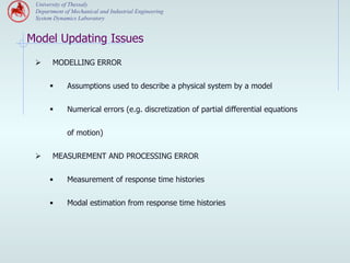
Model Updating Issues
 Ø     MODELLING ERROR


       §    Assumptions used to describe a physical system by a model


       §    Numerical errors (e.g. discretization of partial differential equations


             of motion)


 Ø     MEASUREMENT AND PROCESSING ERROR


       •     Measurement of response time histories


       •     Modal estimation from response time histories
University of Thessaly
       Department of Mechanical and Industrial Engineering
       System Dynamics Laboratory


    Structural Identification - Formulation
       D = {ωr , f ˆr , r = 1,L , m; k = 1,L , N D }
            ˆ                                                    = Available Measured Modal Data

    Μ = Class of Linear Models,             q = structural parameter set to be identified

       ωr (θ ) , f r (θ ) , r = 1,L , m    = Modal data predicted by Model, solving the Eigenvalue Problem

                                       ⎡ K (θ ) − ωr2 M (θ )⎤ f r = 0
                                       ⎣                    ⎦

Problem: Find q values so that model predicted modal data are close to the measured modal data


Measure of fit (Modal Residuals):
                                                       ND
                                                1           [ω r (θ ) − ω r( k ) ]2
                                                                        ˆ
    Modal Frequencies                Jωr (θ ) =        ∑ [ω (k ) ]2                            r = 1, K , m
                                                ND     k =1        ˆr

                                                                                           2   N D = Number of available
                                                       ND
                                                               (k )
                                                              β φ (θ ) − φˆ         (k )
                                                1              r    r              r                 Data sets
       Modeshapes                    Jφr (θ ) =       ∑                        2
                                                ND     k =1           ˆ
                                                                     φr( k )                   For m modesà
                                                                                               maximum 2m objectives
University of Thessaly
 Department of Mechanical and Industrial Engineering
 System Dynamics Laboratory


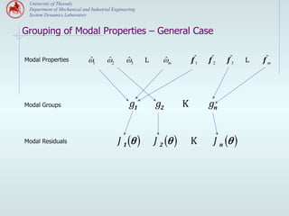
Grouping of Modal Properties – General Case

Modal Properties             ˆ
                             ω1       ˆ
                                      ω2       ˆ
                                               ω3      L      ˆ
                                                              ωm          fˆ
                                                                           1   f ˆ2   f ˆ3   L   f ˆm


Modal Groups                                     g1        g2         K        gn


Modal Residuals                            J 1 (θ )        J 2 (θ )       K      J n (θ )
University of Thessaly
 Department of Mechanical and Industrial Engineering
 System Dynamics Laboratory


Grouping of Modal Properties –Special Case

Modal Properties             ˆ
                             ω1       ˆ
                                      ω2       ˆ
                                               ω3      L           ˆ
                                                                   ωm    fˆ
                                                                          1   f ˆ2     f ˆ3          L   f ˆm


Modal Groups                                      g1                          g2


Modal Residuals                                  J 1 (θ )                     J 2 (θ )
                                                                                              m
                                                            m
                                                 J1 (θ ) = ∑ J ωr (θ )        J 2 (θ ) = ∑ Jφr (θ )
                                                                                              r =1
                                                            r =1


                                                Modal Frequencies                    Modeshapes
University of Thessaly
   Department of Mechanical and Industrial Engineering
   System Dynamics Laboratory


Weighted Modal Residuals Framework
 Find θ that minimizes the weighted modal residuals:

                                                 n
                                J (θ ; w ) = ∑ wi J i (θ )        n = number of modal groups
                                                i =1
                                      n

                                     ∑w =1
                                     i =1
                                            i


                  ˆ
Optimal Solution θ ( w ) depends on the value of the weights       wi

Values of weight factors       w affect optimal θˆ ( w ) which in turn affects model predictions


Problem: Find the most probable (optimal) weight values          ˆ
                                                                 w , based on the measured data
and the norms used to measure the fit between measured and model predicted modal
properties
University of Thessaly
         Department of Mechanical and Industrial Engineering
         System Dynamics Laboratory


      Multi-Objective Framework
       Find θ that simultaneously minimizes the objectives

                                  J (θ )= (J 1 (θ ),J 2 (θ ),K ,J n (θ ))
      Ø  Pareto optimal solutions (Set of alternative solutions).


                                                                             Pareto solutions
                             2


                                                               2
                            J


                                                               x
     Objective Space                      Pareto front                                          Parameter Space


                                              J                               x
                                               1                              1

Ø  All Pareto solutions are acceptable: The characteristics of the Pareto solutions are that the modal residuals cannot
    be improved in any modal property without deteriorating the modal residuals in at least one other modal property.


  Relation to “Weight Modal Residuals Framework” : Varying the values of the weights                  wi
  from 0 to 1, Pareto optimal solutions are alternatively obtained.

  Equivalent Problem: Find the most probable Pareto point and optimal solution to be used for
                            model predictions, based on the measured data
University of Thessaly
  Department of Mechanical and Industrial Engineering
  System Dynamics Laboratory


Optimally Weighted Modal Residuals Method
Most preferred model

Find   θˆpr = θˆ( w ) that minimizes the weighted modal residuals:
                  ˆ
                                                n
                                      ˆ       ˆ
                               J (θ ; w ) = ∑ wi J i (θ )
                                               i =1


selecting the most preferred values of weights to be inversely proportional to the optimal
values of the modal residuals

                                       αi
                           ˆ
                           wi =                 , i = 1,K , n
                                        ˆ( w ))
                                  J i (θ ˆ

The most preferred model for the most preferred weights are obtained by simultaneously
solving the above set of equality equations and the optimization problem


Efficient Solution Strategy: Most preferred model minimizes the sum of the logarithms of
the residuals (Christodoulou and Papadimitriou 2007)
                                                                         n
                              θˆpr = arg min I (θ )             I (θ ) = ∑ αi ln J i (θ )
                                           θ                            i =1
University of Thessaly
   Department of Mechanical and Industrial Engineering
   System Dynamics Laboratory


 Computational Issues – Single Objective Optimization

" Gradient Based Methods
     §  Local methods - Cannot guarantee the estimation of global optimum
     §  Require user-defined initial estimates
     §  Fast convergence – exploit gradient information

" Evolution Strategies (ES)
     §  Global Methods
     §  Do not require user-defined initial estimates
     §  Very slow convergence in the neighborhood of the global optimum

" Hybrid Algorithms (Combine ES and Gradient methods)
     §  Exploit the advantages of ES and Gradient methods
     §  ES explore the parameter space and detect the neighborhood of the global optimum
     §  Gradient methods start from the best estimate of ES and use gradient information to
         accelerate convergence to the global optimum
University of Thessaly
   Department of Mechanical and Industrial Engineering
   System Dynamics Laboratory


 Computational Issues – Multi Objective Optimization

" Strength Pareto Evolutionary Algorithms (SPEA) – [Zitzler and Thiele 1999]
     §  Random initialized population of search points in the parameter space which by
         means of selection, mutation and recombination evolves towards better and better
         regions in the search space
     §  Clustering techniques are used to uniformly distribute points along the Pareto front,
         provided that the values of objectives are of the same order of magnitude along the
         Pareto front
     §  Require user-defined initial estimates
     §  Slow convergence in the neighborhood of the Pareto front

" Normal Boundary Intersection Method (NBI) – [Das and Dennis 1998]
     §    Deterministic algorithms based on gradient methods
     §    Produces an evenly spread of points along the Pareto front
     §    Fast convergence
     §    Computationally expensive for more than 3 objectives
University of Thessaly
  Department of Mechanical and Industrial Engineering
  System Dynamics Laboratory


Computational Issues – Gradients of Objectives
In order to guarantee the convergence of the gradient-based optimization methods, the
gradients of the objective functions with respect to the parameter set θ has to be estimated
accurately

Nelson’s Method

Gradient of eigenvalue and eigenvector of a mode is computed using information from the
eigenvalue and eigenvector of the same mode


Adjoint Formulation

The computational cost is independent of number of parameters.
For each mode a solution of a linear system of algebraic equations is required

Hessian of objectives
University of Thessaly
                       Department of Mechanical and Industrial Engineering
                       System Dynamics Laboratory


                   Polymylos Bridge - Instrumentation


                                                                                                                                             Instrumented with an array of 24
                                                                                                                                             accelerometers optimally placed
                                                                                                                                              on the deck and the base of the
                                                                                                                                                   columns and bearings


                                                                                                                                                                                                                                                    2

                                                                                                                                                                                                                                             14         1
                                                                                                                                                                                                                                               13
                                                                                                                                                                                                                              3
                                                                                                                                                                                                                                   15
                                   B2RV 40                    M2RV 10                     A2RV40
                                                                                                                                                                                                         5                    16
                                                                                                                 SRV 100                                                                                         17
            T3RT 100                                                         M2RT 10                                            T1RT 100                                                 9
                                             B2RT 40                                               A2RT 40                                                                                                            4
                                                                                                                                                                                              19        18
                                                                                                                  SRT 100                                                     10
                       ΠΟΛΥΜΥΛΟΣ                                                                                                                                                   21   20
                                                             M2 LL 10                                                                                                    12
  U3LL100                                                                                                                                                                     22
                                                                                                                                           U1LV 100              02423                                       6
                                                                        M2LV 10                                                                                               11
                                             B2LV 40                                           A2LV 40                      U1LL 100
                                                                                                             SLV 100                                           -10                                  7                     8             50
U3LV 100                                                                            Βάση                                                   U1RT 100   z-axis
            U3RT 100                                         U2LV 40                                                                                           -20
                                                                                  Πυλώνα M2
                                                                                                                                                                                                                  0
   Aκρόβαθρο T2                                                               U2LL 40
                                                                                                                                                               -30
                                                       35m                              35m          30m                        Aκρόβαθρο T1
                               30m                             U2LT 40                                                                                                                  -50
                                                                                                                                                               -750
                                                                                                                                                                -755                               x-axis
                                                                                                                                                                 -760
                                                                                                                                                      y-axis
University of Thessaly
 Department of Mechanical and Industrial Engineering
 System Dynamics Laboratory


Polymylos Bridge – Operational Modal Analysis


                                                                                                                                                                  Damping
                                                       No                          Identified Modes                                   Hz
                                                                                                                                                                  Ratios (%)
      Modal Identification Software                     1                                1st longitudinal                             1.19                                    5.56
                                                        2                                 2nd transverse                              1.12                                    1.97
                                                        3                          1st bending (deck)                                 2.13                                    0.60
                                                        4                          2nd bending (deck)                                 3.07                                    0.43
                                                        5                                  4th transverse                             4.07                                    0.76
                                                        6                          3rd bending (deck)                                 6.65                                    0.45


                                                                                                                                                                                                         1
                                                                                         Mode 1: 2.131 Hz, zeta=1.260%                                                  Mode 2: 2.225 Hz, zeta=3.737%
                                                                                                                                                                                                             7
                                                                                                                                  6                                                                                   6

                                                                                             4
                                                                                                  11
                                                                               5                                         8                                                                                   8
                                                                                   13
                                                                                                           2
                                                                                                           3                                                                                3
                                                                                                                                                                                            2
                                                                                                                10
                                                                                                                9                                                                                9
                                                                                                                                                                                                 10

                                                                                                  12                 1                                                       4 12
                                                                                                                         7
                                                                   0                14
                                                                                                                                                  0           5   14               11

                                                                 -10      15                                                 50                 -10      15
                                                                                                                                                                   13                                            50


                                                        z-axis


                                                                                                                                       z-axis
                                                                 -20                                                                            -20
                                                                                                                 0                                                                                   0
                                                                 -30                                                                            -30

                                                                                            -50                                                                              -50
                                                                 -750
                                                                  -755                                 x-axis                                   -750
                                                                                                                                                 -755                                   x-axis
                                                                   -760                                                                           -760
                                                       y-axis                                                                          y-axis


                                                                                                                                                                                                                 6
                                                                                         Mode 3: 3.074 Hz, zeta=1.035%                                                  Mode 4: 4.095 Hz, zeta=1.435%
                                                                                                                     1
                                                                                                                         7        6

                                                                                                                                                                                                         1
                                                                                             4
                                                                               5
                                                                                   13             11                     8                                                                                   7

                                                                                                           3                                                                                     2
                                                                                                           2                                                                                3
                                                                                                                9                                                       12                                        8
                                                                                                                10                                                           4                   10
                                                                                                                                                                                                 9
                                                                                                                                                                                   11
                                                                                                  12
                                                                                                                                                              5
                                                                   0                                                                              0                13
                                                                                   14                                                                             14

                                                                 -10      15                                                 50                 -10      15                                                      50
                                                        z-axis


                                                                                                                                       z-axis
                                                                 -20                                                                            -20
                                                                                                                 0                                                                                   0
                                                                 -30                                                                            -30

                                                                                            -50                                                                              -50
                                                                 -750
                                                                  -755                                 x-axis                                   -750
                                                                                                                                                 -755                                   x-axis
                                                                   -760                                                                           -760
                                                       y-axis                                                                          y-axis
University of Thessaly
 Department of Mechanical and Industrial Engineering
 System Dynamics Laboratory


Polymylos Bridge – Finite Element Model
   Finite Element Model Updating using Multi-Objective Identification

   Finite element model of 228
   beam elements (1038 DOF)                                 3 parameter FE model

                                J2
                                θ12
                                 1
    z                                                  θ1    θ2
            x                                                                      θ1
        y                                                                θ3


  Model Updating Software
University of Thessaly
                        Department of Mechanical and Industrial Engineering
                        System Dynamics Laboratory


                Polymylos Bridge - Model Updating Results
                      3 parameters Multi-Objective model updating using 3 modes
                                                                                                                                                                                                                                         ND
                                                                                                                                                                                                                                  1          [ωr (q ) − ωr k ) ]2
                                                                                                                                                                                                                                                           ˆ(
                                                                                                                                                                                                                    J1 (q ) =           ∑
                                                                                                                                                                                                                                  ND              [ωr k ) ]2
                                                                                                                                                                                                                                                   ˆ(
                                                           Objective and parameters space
                                                                                                                                                                                                                                        k =1
                                                                                                                                                                                                                                                                                 2
                                                                                                                                                                                                                                       ND                        ˆ
                                                                                                                                                                                                                                              β r( k )φr (q ) − φr( k )
                                                                                                                                                                                                                                  1
        0.072                                                                                                     1.8                                                                                                J 2 (q ) =        ∑                                2
                                                                              Pareto Solutions                                                             20
                                                                                                                                                                                    19                                            ND   k =1                    ˆ
                                                                                                                                                                                                                                                              φr( k )
         0.07                                                                 w=1                                                                                                        18
                    1                                                                                             1.6
                    2                                                                                                                                                                         17
        0.068        3                                                                                                                                                                             16   Equally weighted method parameter values
                      4                                                                                                                        Pareto Solutions
                                                                                                                  1.4
                                                                                                                                                                                                                   θ1 (E bearings)   3.6872
                                                                                                              2

                      5
2


                                                                                                                                                                                               15
                                                                                                              θ
J


                        6                                                                                                                      w=1
        0.066
                         7
                             8                                                                                                                                                                     14                 θ2 (E deck)    1.1293
                                 9                                                                                1.2                                                                     13
        0.064
                                     10
                                          11 12                                                                                                                                     12                                θ3 (E pier)    0.6425
                                                13 14                                                                                                           10      11
                                                      15 16                     17 18       19        20                                  7 8
                                                                                                                                                        9                                                       J1(mode frequencies) 0.0347
        0.062                                                                                                      1            123 4 5 6
                0      0.02               0.04    0.06             0.08         0.1      0.12     0.14              3.3           3.4      3.5                  3.6           3.7              3.8                J2 (mode shapes)   0.0635
                                                           J                                                                                           θ
                                                           1                                                                                               1                                                       3.8
                                                                                                                                                                                                                   3.6
                                                                                                                                                                                                                   3.4
           1                                                                                                       1
                                                                                                                                                                                                                   3.2
                                                                                                                                                                                                                                                                                 θ
                                                                                                                                                                                                                     3                                                            1
                                                                                                                                                                      Pareto Solutions
                             12 3 4 5                                                                                       25
                                                                                                                            14
                                                                                                                            3                                                                                      2.8                                                           θ
                                                                                                                                                                                                                                                                                  2
          0.8                         6 7                                                                         0.8         67                                      w=1                                          2.6
                                                       8       9                                                               89                                                                                                                                                θ
                                                                         10                                                      10                                                                                2.4                                                            3
                                                                                    11                                            11                                                                               2.2                                                           θw =1
                                                                                            12                                      12


                                                                                                                                                                                                         θ value
          0.6                                                                                         13          0.6                     13                                                                         2
                                             Pareto Solutions                                                                                                                                                      1.8
                                                                                                         14                                     14
    3


                                                                                                              3
θ


                                                                                                              θ


                                             w=1                                                       15                                              15                                                          1.6
          0.4                                                                                            16       0.4                                            16                                                1.4
                                                                                                      17                                                                 17                                        1.2
                                                                                                 18                                                                             18                                   1
                                                                                            19                                                                                        19
          0.2                                                      20                                             0.2                                                                20                            0.8
                                                                                                                                                                                                                   0.6
                                                                                                                                                                                                                   0.4
           0                                                                                                       0                                                                                               0.2
            3.3                  3.4             3.5                    3.6           3.7             3.8               1                1.2           1.4                1.6                  1.8
                                                                                                                                                                                                                              5          10              15                 20
                                                           θ                                                                                           θ                                                                                   # of solutions
                                                               1                                                                                           2
University of Thessaly
 Department of Mechanical and Industrial Engineering
 System Dynamics Laboratory


  Conclusions
Ø    Model updating algorithms were proposed to compute all Pareto optimal models
      consistent with measured data and the norms used to measure the fit between the
      measured and model predicted modal properties.
Ø    The equivalence between the multi-objective identification and the weighted modal
      residuals method was established.
Ø    Hybrid algorithms based on evolution strategies and gradient methods are well-suited
      optimization tools for solving the resulting optimization problem and identifying the global
      optimum from multiple local ones.
Ø    NBI algorithms are well-suited multi-objective optimization tools for solving the multi-
      objective identification problem. NBI effectively computes the useful identifiable part of
      the Pareto front.
Ø    The computational cost for estimating analytically the gradients of the objectives is shown
      to be independent of the number of structural model parameters.

Multi-Objective Optimization Algorithms for Finite Element Model Updating. Ntotsios and Papadimitriou.

  • 1.
    University of Thessaly Departmentof Mechanical and Industrial Engineering System Dynamics Laboratory Multi-Objective Optimization Algorithms for Finite Element Model Updating E. Ntotsios, C. Papadimitriou University of Thessaly Greece
  • 2.
    University of Thessaly Department of Mechanical and Industrial Engineering System Dynamics Laboratory Outline Ø  STRUCTURAL IDENTIFICATION USING MEASURED MODAL DATA §  Weighted Modal Residuals Framework §  Multi-Objective Framework §  Optimally Weighted Modal Residuals Method Ø  COMPUTATIONAL ISSUES §  Single-Objective Optimization §  Multi-Objective Optimization §  Gradient and Hessian of Objectives Ø  ILUSTATIVE EXAMPLE •  Structural Identification of a Full Scale Bridge Using Ambient Vibration Measurements Ø  CONCLUSIONS
  • 3.
    University of Thessaly Department of Mechanical and Industrial Engineering System Dynamics Laboratory Model Updating Issues Ø  MODELLING ERROR §  Assumptions used to describe a physical system by a model §  Numerical errors (e.g. discretization of partial differential equations of motion) Ø  MEASUREMENT AND PROCESSING ERROR •  Measurement of response time histories •  Modal estimation from response time histories
  • 4.
    University of Thessaly Department of Mechanical and Industrial Engineering System Dynamics Laboratory Structural Identification - Formulation D = {ωr , f ˆr , r = 1,L , m; k = 1,L , N D } ˆ = Available Measured Modal Data Μ = Class of Linear Models, q = structural parameter set to be identified ωr (θ ) , f r (θ ) , r = 1,L , m = Modal data predicted by Model, solving the Eigenvalue Problem ⎡ K (θ ) − ωr2 M (θ )⎤ f r = 0 ⎣ ⎦ Problem: Find q values so that model predicted modal data are close to the measured modal data Measure of fit (Modal Residuals): ND 1 [ω r (θ ) − ω r( k ) ]2 ˆ Modal Frequencies Jωr (θ ) = ∑ [ω (k ) ]2 r = 1, K , m ND k =1 ˆr 2 N D = Number of available ND (k ) β φ (θ ) − φˆ (k ) 1 r r r Data sets Modeshapes Jφr (θ ) = ∑ 2 ND k =1 ˆ φr( k ) For m modesà maximum 2m objectives
  • 5.
    University of Thessaly Department of Mechanical and Industrial Engineering System Dynamics Laboratory Grouping of Modal Properties – General Case Modal Properties ˆ ω1 ˆ ω2 ˆ ω3 L ˆ ωm fˆ 1 f ˆ2 f ˆ3 L f ˆm Modal Groups g1 g2 K gn Modal Residuals J 1 (θ ) J 2 (θ ) K J n (θ )
  • 6.
    University of Thessaly Department of Mechanical and Industrial Engineering System Dynamics Laboratory Grouping of Modal Properties –Special Case Modal Properties ˆ ω1 ˆ ω2 ˆ ω3 L ˆ ωm fˆ 1 f ˆ2 f ˆ3 L f ˆm Modal Groups g1 g2 Modal Residuals J 1 (θ ) J 2 (θ ) m m J1 (θ ) = ∑ J ωr (θ ) J 2 (θ ) = ∑ Jφr (θ ) r =1 r =1 Modal Frequencies Modeshapes
  • 7.
    University of Thessaly Department of Mechanical and Industrial Engineering System Dynamics Laboratory Weighted Modal Residuals Framework Find θ that minimizes the weighted modal residuals: n J (θ ; w ) = ∑ wi J i (θ ) n = number of modal groups i =1 n ∑w =1 i =1 i ˆ Optimal Solution θ ( w ) depends on the value of the weights wi Values of weight factors w affect optimal θˆ ( w ) which in turn affects model predictions Problem: Find the most probable (optimal) weight values ˆ w , based on the measured data and the norms used to measure the fit between measured and model predicted modal properties
  • 8.
    University of Thessaly Department of Mechanical and Industrial Engineering System Dynamics Laboratory Multi-Objective Framework Find θ that simultaneously minimizes the objectives J (θ )= (J 1 (θ ),J 2 (θ ),K ,J n (θ )) Ø  Pareto optimal solutions (Set of alternative solutions). Pareto solutions 2 2 J x Objective Space Pareto front Parameter Space J x 1 1 Ø  All Pareto solutions are acceptable: The characteristics of the Pareto solutions are that the modal residuals cannot be improved in any modal property without deteriorating the modal residuals in at least one other modal property. Relation to “Weight Modal Residuals Framework” : Varying the values of the weights wi from 0 to 1, Pareto optimal solutions are alternatively obtained. Equivalent Problem: Find the most probable Pareto point and optimal solution to be used for model predictions, based on the measured data
  • 9.
    University of Thessaly Department of Mechanical and Industrial Engineering System Dynamics Laboratory Optimally Weighted Modal Residuals Method Most preferred model Find θˆpr = θˆ( w ) that minimizes the weighted modal residuals: ˆ n ˆ ˆ J (θ ; w ) = ∑ wi J i (θ ) i =1 selecting the most preferred values of weights to be inversely proportional to the optimal values of the modal residuals αi ˆ wi = , i = 1,K , n ˆ( w )) J i (θ ˆ The most preferred model for the most preferred weights are obtained by simultaneously solving the above set of equality equations and the optimization problem Efficient Solution Strategy: Most preferred model minimizes the sum of the logarithms of the residuals (Christodoulou and Papadimitriou 2007) n θˆpr = arg min I (θ ) I (θ ) = ∑ αi ln J i (θ ) θ i =1
  • 10.
    University of Thessaly Department of Mechanical and Industrial Engineering System Dynamics Laboratory Computational Issues – Single Objective Optimization " Gradient Based Methods §  Local methods - Cannot guarantee the estimation of global optimum §  Require user-defined initial estimates §  Fast convergence – exploit gradient information " Evolution Strategies (ES) §  Global Methods §  Do not require user-defined initial estimates §  Very slow convergence in the neighborhood of the global optimum " Hybrid Algorithms (Combine ES and Gradient methods) §  Exploit the advantages of ES and Gradient methods §  ES explore the parameter space and detect the neighborhood of the global optimum §  Gradient methods start from the best estimate of ES and use gradient information to accelerate convergence to the global optimum
  • 11.
    University of Thessaly Department of Mechanical and Industrial Engineering System Dynamics Laboratory Computational Issues – Multi Objective Optimization " Strength Pareto Evolutionary Algorithms (SPEA) – [Zitzler and Thiele 1999] §  Random initialized population of search points in the parameter space which by means of selection, mutation and recombination evolves towards better and better regions in the search space §  Clustering techniques are used to uniformly distribute points along the Pareto front, provided that the values of objectives are of the same order of magnitude along the Pareto front §  Require user-defined initial estimates §  Slow convergence in the neighborhood of the Pareto front " Normal Boundary Intersection Method (NBI) – [Das and Dennis 1998] §  Deterministic algorithms based on gradient methods §  Produces an evenly spread of points along the Pareto front §  Fast convergence §  Computationally expensive for more than 3 objectives
  • 12.
    University of Thessaly Department of Mechanical and Industrial Engineering System Dynamics Laboratory Computational Issues – Gradients of Objectives In order to guarantee the convergence of the gradient-based optimization methods, the gradients of the objective functions with respect to the parameter set θ has to be estimated accurately Nelson’s Method Gradient of eigenvalue and eigenvector of a mode is computed using information from the eigenvalue and eigenvector of the same mode Adjoint Formulation The computational cost is independent of number of parameters. For each mode a solution of a linear system of algebraic equations is required Hessian of objectives
  • 13.
    University of Thessaly Department of Mechanical and Industrial Engineering System Dynamics Laboratory Polymylos Bridge - Instrumentation Instrumented with an array of 24 accelerometers optimally placed on the deck and the base of the columns and bearings 2 14 1 13 3 15 B2RV 40 M2RV 10 A2RV40 5 16 SRV 100 17 T3RT 100 M2RT 10 T1RT 100 9 B2RT 40 A2RT 40 4 19 18 SRT 100 10 ΠΟΛΥΜΥΛΟΣ 21 20 M2 LL 10 12 U3LL100 22 U1LV 100 02423 6 M2LV 10 11 B2LV 40 A2LV 40 U1LL 100 SLV 100 -10 7 8 50 U3LV 100 Βάση U1RT 100 z-axis U3RT 100 U2LV 40 -20 Πυλώνα M2 0 Aκρόβαθρο T2 U2LL 40 -30 35m 35m 30m Aκρόβαθρο T1 30m U2LT 40 -50 -750 -755 x-axis -760 y-axis
  • 14.
    University of Thessaly Department of Mechanical and Industrial Engineering System Dynamics Laboratory Polymylos Bridge – Operational Modal Analysis Damping No Identified Modes Hz Ratios (%) Modal Identification Software 1 1st longitudinal 1.19 5.56 2 2nd transverse 1.12 1.97 3 1st bending (deck) 2.13 0.60 4 2nd bending (deck) 3.07 0.43 5 4th transverse 4.07 0.76 6 3rd bending (deck) 6.65 0.45 1 Mode 1: 2.131 Hz, zeta=1.260% Mode 2: 2.225 Hz, zeta=3.737% 7 6 6 4 11 5 8 8 13 2 3 3 2 10 9 9 10 12 1 4 12 7 0 14 0 5 14 11 -10 15 50 -10 15 13 50 z-axis z-axis -20 -20 0 0 -30 -30 -50 -50 -750 -755 x-axis -750 -755 x-axis -760 -760 y-axis y-axis 6 Mode 3: 3.074 Hz, zeta=1.035% Mode 4: 4.095 Hz, zeta=1.435% 1 7 6 1 4 5 13 11 8 7 3 2 2 3 9 12 8 10 4 10 9 11 12 5 0 0 13 14 14 -10 15 50 -10 15 50 z-axis z-axis -20 -20 0 0 -30 -30 -50 -50 -750 -755 x-axis -750 -755 x-axis -760 -760 y-axis y-axis
  • 15.
    University of Thessaly Department of Mechanical and Industrial Engineering System Dynamics Laboratory Polymylos Bridge – Finite Element Model Finite Element Model Updating using Multi-Objective Identification Finite element model of 228 beam elements (1038 DOF) 3 parameter FE model J2 θ12 1 z θ1 θ2 x θ1 y θ3 Model Updating Software
  • 16.
    University of Thessaly Department of Mechanical and Industrial Engineering System Dynamics Laboratory Polymylos Bridge - Model Updating Results 3 parameters Multi-Objective model updating using 3 modes ND 1 [ωr (q ) − ωr k ) ]2 ˆ( J1 (q ) = ∑ ND [ωr k ) ]2 ˆ( Objective and parameters space k =1 2 ND ˆ β r( k )φr (q ) − φr( k ) 1 0.072 1.8 J 2 (q ) = ∑ 2 Pareto Solutions 20 19 ND k =1 ˆ φr( k ) 0.07 w=1 18 1 1.6 2 17 0.068 3 16 Equally weighted method parameter values 4 Pareto Solutions 1.4 θ1 (E bearings) 3.6872 2 5 2 15 θ J 6 w=1 0.066 7 8 14 θ2 (E deck) 1.1293 9 1.2 13 0.064 10 11 12 12 θ3 (E pier) 0.6425 13 14 10 11 15 16 17 18 19 20 7 8 9 J1(mode frequencies) 0.0347 0.062 1 123 4 5 6 0 0.02 0.04 0.06 0.08 0.1 0.12 0.14 3.3 3.4 3.5 3.6 3.7 3.8 J2 (mode shapes) 0.0635 J θ 1 1 3.8 3.6 3.4 1 1 3.2 θ 3 1 Pareto Solutions 12 3 4 5 25 14 3 2.8 θ 2 0.8 6 7 0.8 67 w=1 2.6 8 9 89 θ 10 10 2.4 3 11 11 2.2 θw =1 12 12 θ value 0.6 13 0.6 13 2 Pareto Solutions 1.8 14 14 3 3 θ θ w=1 15 15 1.6 0.4 16 0.4 16 1.4 17 17 1.2 18 18 1 19 19 0.2 20 0.2 20 0.8 0.6 0.4 0 0 0.2 3.3 3.4 3.5 3.6 3.7 3.8 1 1.2 1.4 1.6 1.8 5 10 15 20 θ θ # of solutions 1 2
  • 17.
    University of Thessaly Department of Mechanical and Industrial Engineering System Dynamics Laboratory Conclusions Ø  Model updating algorithms were proposed to compute all Pareto optimal models consistent with measured data and the norms used to measure the fit between the measured and model predicted modal properties. Ø  The equivalence between the multi-objective identification and the weighted modal residuals method was established. Ø  Hybrid algorithms based on evolution strategies and gradient methods are well-suited optimization tools for solving the resulting optimization problem and identifying the global optimum from multiple local ones. Ø  NBI algorithms are well-suited multi-objective optimization tools for solving the multi- objective identification problem. NBI effectively computes the useful identifiable part of the Pareto front. Ø  The computational cost for estimating analytically the gradients of the objectives is shown to be independent of the number of structural model parameters.