The document discusses multi-objective optimization and various techniques used to solve multi-objective problems. It introduces concepts like Pareto optimality and Pareto frontier. It then describes various solution methods like weighted sum, normal boundary intersection, goal programming, and Pareto genetic algorithms. Genetic algorithms use concepts like fitness, reproduction, and Pareto set filtering to evolve a population towards the Pareto optimal frontier while satisfying constraints.

1. MULTI OBJECTIVE OPTIMIZATION AND TRADE
OFFS USING PARETO OPTIMALITY
Amogh Mundhekar
Nikhil Aphale
[University at Buffalo, SUNY]

2. Multi-Objective Optimization

3. Multi-Objective Optimization

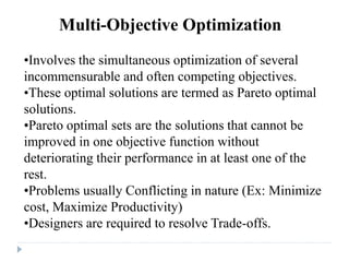
4. Multi-Objective Optimization
•Involves the simultaneous optimization of several
incommensurable and often competing objectives.
•These optimal solutions are termed as Pareto optimal
solutions.
•Pareto optimal sets are the solutions that cannot be
improved in one objective function without
deteriorating their performance in at least one of the
rest.
•Problems usually Conflicting in nature (Ex: Minimize
cost, Maximize Productivity)
•Designers are required to resolve Trade-offs.

5. Pareto Optimal means:
“Take from Peter to pay Paul”

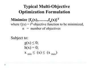
6. Typical Multi-Objective
Optimization Formulation
Minimize {f1(x),…….,fn(x)}T
where fi(x) = ith objective function to be minimized,
n = number of objectives
Subject to:
g(x) ≤ 0;
h(x) = 0;
x min ≤ (x) ≤ (x max)

7. Basic Terminology
 Search space or design space is the set of all possible
combinations of the design variables.
 Pareto Optimal Solution achieves a trade off. They are
solutions for which any improvement in one objective results in
worsening of atleast one other objective.
 Pareto Optimal Set: Pareto Optimal Solution is not unique,
there exists a set of solutions known as the Pareto Optimal Set.
It represents a complete set of solutions for a Multi-Objective
Optimization (MOO).
 Pareto Frontier: A plot of entire Pareto set in the Design
Objective Space (with design objectives plotted along each
axis) gives a Pareto Frontier.

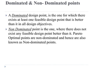
8. Dominated & Non- Dominated points
 A Dominated design point, is the one for which there
exists at least one feasible design point that is better
than it in all design objectives.
 Non Dominated point is the one, where there does not
exist any feasible design point better than it. Pareto
Optimal points are non-dominated and hence are also
known as Non-dominated points.

9. Challenges in the Multi Objective
Optimization problem.
Challenge 1: Populate the Pareto Set
Challenge 2: Select the Best Solution
Challenge 3: Find the corresponding Design Variables

10. Solution methods for Challenge 1
Methods discusses in earlier lectures:
 Random Sampling
 Weighting Method
 Distance Method
 Constrained Trade-off method

11. Solution methods for Challenge 1
Methods discusses to be discussed today:
 Random Sampling
 Weighting Method
 Distance Method
 Constrained Trade-off method
 Normal Boundary Intersection method
 Goal Programming
 Pareto Genetic Algorithm

12. Weighted Sum Approach

13. Weighted Sum Approach
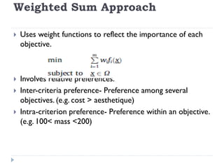
 Uses weight functions to reflect the importance of each
objective.
 Involves relative preferences.
 Inter-criteria preference- Preference among several
objectives. (e.g. cost > aesthetique)
 Intra-criterion preference- Preference within an objective.
(e.g. 100< mass <200)

14. Drawbacks of Weighted sum method
 Finding points on the Pareto front by varying the weighting
coefficients yields incorrect outputs.
 Small changes in ‘w’ may cause dramatic changes in the
objective vectors. Whereas large changes in ‘w’ may result in
almost unnoticeable changes in the objective vectors. This
makes the relation between weights and performance very
complicated and non-intuitive.
 Uneven sampling of the Pareto front.
 Requires Scaling.

15. Drawbacks of Weighted sum method..
 For an even spread of the weights, the optimal solutions in the
criterion space are usually not evenly distributed
 Weighted sum method is essentially subjective, in that a
Decision Maker needs to provide the weights.
 This approach cannot identify all non-dominated solutions.
Only solutions located on the convex part of the Pareto front
can be found. If the Pareto set is not convex, the Pareto points
on the concave parts of the trade-off surface will be missed.
 Does not provide the means to effectively specify intra-
criterion preferences.

16. Normal Boundary
Intersections (NBI)

17. Normal Boundary Intersections (NBI)
 NBI is a solution methodology developed by Das and Dennis
(1998) for generating Pareto surface in non-linear
multiobjective optimization problems.
 This method is independent of the relative scales of the
objective functions and is successful in producing an evenly
distributed set of points in the Pareto surface given an evenly
distributed set of parameters, which is an advantage compared
to the most common multiobjective approaches—weighting
method and the ε-constraint method.
 A method for finding several Pareto optimal points for a
general nonlinear multi criteria optimization problem, aimed at
capturing the tradeoff among the various conflicting objectives.

18. Normal Boundary Intersections (NBI)
 NBI is a solution methodology developed by Das and Dennis
(1998) for generating Pareto surface in non-linear
multiobjective optimization problems.
 This method is independent of the relative scales of the
objective functions and is successful in producing an evenly
distributed set of points in the Pareto surface given an evenly
distributed set of parameters, which is an advantage compared
to the most common multiobjective approaches—weighting
method and the ε-constraint method.
 A method for finding several Pareto optimal points for a
general nonlinear multi criteria optimization problem, aimed at
capturing the tradeoff among the various conflicting objectives.

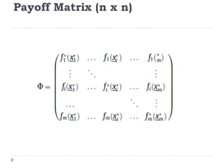
19. Payoff Matrix (n x n)

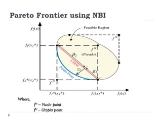
20. Pareto Frontier using NBI
Where,
fN – Nadir point
fU – Utopia point

21. Convex Hull of Individual Minima (CHIM)
 The set of points in objective space that are convex
combinations of each row of payoff table, is referred to as the
Convex Hull of Individual Minima (CHIM).

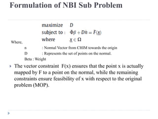
22. Formulation of NBI Sub Problem
Where,
n : Normal Vector from CHIM towards the origin
D : Represents the set of points on the normal.
Beta : Weight
 The vector constraint F(x) ensures that the point x is actually
mapped by F to a point on the normal, while the remaining
constraints ensure feasibility of x with respect to the original
problem (MOP).

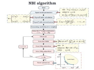
23. NBI algorithm

24. Advantages of NBI
 Finds a uniform spread of Pareto points.
 NBI improves on other traditional methods like goal
programming in the sense that it never requires any prior
knowledge of 'feasible goals'.
 It improves on multilevel optimization techniques from
the tradeoff standpoint, since multilevel techniques
usually can only improve only a few of the 'most
important' objectives, leaving no compromise for the rest.

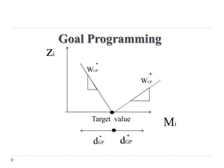
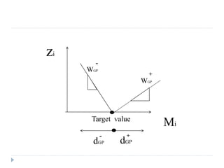
25. Goal Programming
zi
-
WGP
+
WGP
Target value
Mi
- +
dGP dGP

26. History
Goal programming was first used by Charnes
and Cooper in 1955.
The first engineering application of goal
programming, was by Ignizio in 1962:
Designing and placing of the antennas on the
second stage of the Saturn V.

27. How this method works?
Requirements:
1) Choosing either Max or Min the objective
2) Setting a target or a goal value for each objective
3) Designer specifies -
WGP & WGP +
Therefore, indicate penalties for deviating from either sides
Basic principle:
Minimize the deviation of each
design objective from its target value
- +
Deviational variables dGP & dGP

28. zi
-
WGP
+
WGP
Target value
Mi
- +
dGP dGP

29. The Game

30. Advantages and disadvantages
1) Simplicity and ease of use
2) It is better than weighted sum method because the
designer specify two different values of weights for
each objective on the two sides of the target value
1) Specifying weights for the designer preference is not
easy
2) What about…?

31. Testing for Pareto
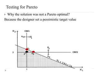
Why the solution was not a Pareto optimal?
Because the designer set a pessimistic target value

32. Larbani & Aounini method
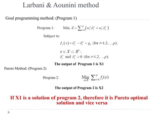
Goal programming method: (Program 1)
The output of Program 1 is X1
Pareto Method: (Program 2)
The output of Program 2 is X2
If X1 is a solution of program 2, therefore it is Pareto optimal
solution and vice versa

33. Multiobjective Optimization
using Pareto Genetic
Algorithm

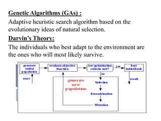
34. Genetic Algorithms (GAs) :
Adaptive heuristic search algorithm based on the
evolutionary ideas of natural selection.
Darvin’s Theory:
The individuals who best adapt to the environment are
the ones who will most likely survive.

35. Important Concepts in GAs
1. Fitness:
 Each nondominated point in a model should be equally
important and considered an optimal goal.
 Nondominated rank procedure.

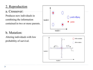
36. 2. Reproduction
a. Crossover:
Produces new individuals in
combining the information
contained in two or more parents.
b. Mutation:
Altering individuals with low
probability of survival.

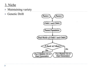
37. 3. Niche
 Maintaining variety
 Genetic Drift

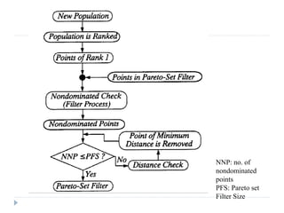
38. 4. Pareto Set Filter
 Reproduction cannot guarantee that best characteristics of
the parents are inherited by their next generation.
 Some of them maybe Pareto optimal points
 Filter pools nondominated points ranked 1 at each
generation and drops dominated points.

39. NNP: no. of
nondominated
points
PFS: Pareto set
Filter Size

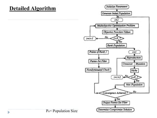
40. Detailed Algorithm
Pn= Population Size

41. Constrained Multiobjective Optimization via GAs
 Transform a constrained optimization problem into an
unconstrained one via penalty function method.
Minimize F(x)
subject to,
g(x) <= 0
h(x) = 0
Transform to,
Minimize Φ(x) = F(x) + rp P(x)
 A penalty term is added to the fitness of an infeasible
point so that its fitness never attains that of a feasible
point.

42. Fuzzy Logic (FL) Penalty Function Method
 Derives from the fact that classes and concepts for
natural phenomenon tend to be fuzzy instead of crisp.
 Fuzzy Set
 A point is identified with its degree of membership in that set.
A fuzzy set A in X( a collection of objects) is defined as,
μ mapping from X to unit interval [0,1] called as membership
A :
function
 0: worst possible case
 1: best possible case


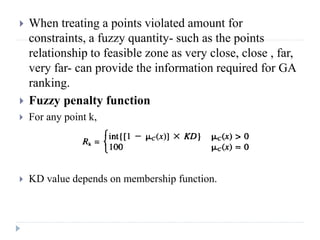
43.  When treating a points violated amount for
constraints, a fuzzy quantity- such as the points
relationship to feasible zone as very close, close , far,
very far- can provide the information required for GA
ranking.
 Fuzzy penalty function
 For any point k,
 KD value depends on membership function.

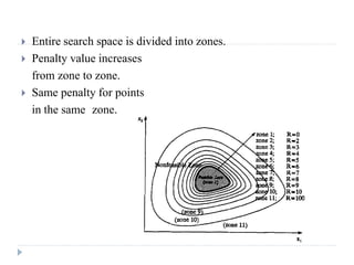
44.  Entire search space is divided into zones.
 Penalty value increases
from zone to zone.
 Same penalty for points
in the same zone.

45.  Advantages of GAs
 Doesn’t require gradient information
 Only input information required from the given problem is
fitness of each point in present model population.
 Produce multiple optima rather than single local optima.
 Disadvantages
 Not good when Function evaluation is expensive.
 Large computations required.