Ch3_Z-transform.pdf

Discrete-Time Signal Processing, 2/E by Alan V. Oppenheim and Ronald W. Schafer
Chapter 3 The Z-Transorm
Def: Z-transform operator
Two-side or bilateral z-transform
One-side or unilateral z-transform
3.1 z-Transform
Recall the Fourier transform of a sequence x[n] in Chapter 2 was
defined as
∑
∞
−∞
=
ω
−
ω
=
n
n
j
j
e
]
n
[
x
)
e
(
X
The z-transform of a sequence x[n] is defined as
∑
∞
−∞
=
−
=
n
n
z
]
n
[
x
)
z
(
X
∑
∞
=
−
=
0
n
n
z
]
n
[
x
)
z
(
X
)
z
(
X
z
]
n
[
x
]}
n
[
x
{
Z
n
n
=
= ∑
∞
−∞
=
−
The correspondence between a sequence and its z-transform is indicated by
the notation
)
z
(
X
]
n
[
x Z
⎯→
←

More generally, we can express the complex variable z in polar form as
ω
= j
re
z
For |z|=1, the z-transorm corresponds to the Fourier transform
∑
∞
−∞
=
−
ω
ω
=
n
n
j
j
)
re
](
n
[
x
)
re
(
X
)
z
(
X
z
]
n
[
x
]}
n
[
x
{
Z
n
n
=
= ∑
∞
−∞
=
−
∑
∞
−∞
=
ω
−
−
ω
=
n
n
j
n
j
e
)
r
]
n
[
x
(
)
re
(
X
The equation can be interpreted as the Fourier transform of the product of
the original sequence x[n] and the exponential sequence r-n. Obviously, for
r=1, the z-transform reduces to the Fourier transform of x[n].

Figure 3.1 The unit circle in the
complex z-plane
∞
<
∑
∞
−∞
=
−
n
n
|
z
||
]
n
[
x
|
Convergence of z-transform requires
∞
<
∑
∞
−∞
=
−
n
n
|
r
]
n
[
x
|
Convergence of Fourier transform
requires
∞
<
∑
∞
−∞
=
n
|
]
n
[
x
|
, i.e., |z|=1

For any given sequences, the set of values of z for which the z-transform
converges is called the region of convergence, abbreviated as ROC.
∞
<
∑
∞
−∞
=
−
n
n
|
r
]
n
[
x
|
Because of the multiplication of the sequence by the real exponential r-n, it
is possible for the z-transform to converge even if the Fourier transfrom
does not. For example, the sequence x[n] = u[n] is not absolutely
summable, and its Fourier transform does not converge absolutely.
However, r-nu[n] is absolutely summable for r>1.

Region of Converge (ROC)
Definition : a set of values z for |X(z)| < ∞ , which depends only on |z|
∞
<
∑
∞
−∞
=
−
n
n
|
z
||
]
n
[
x
|

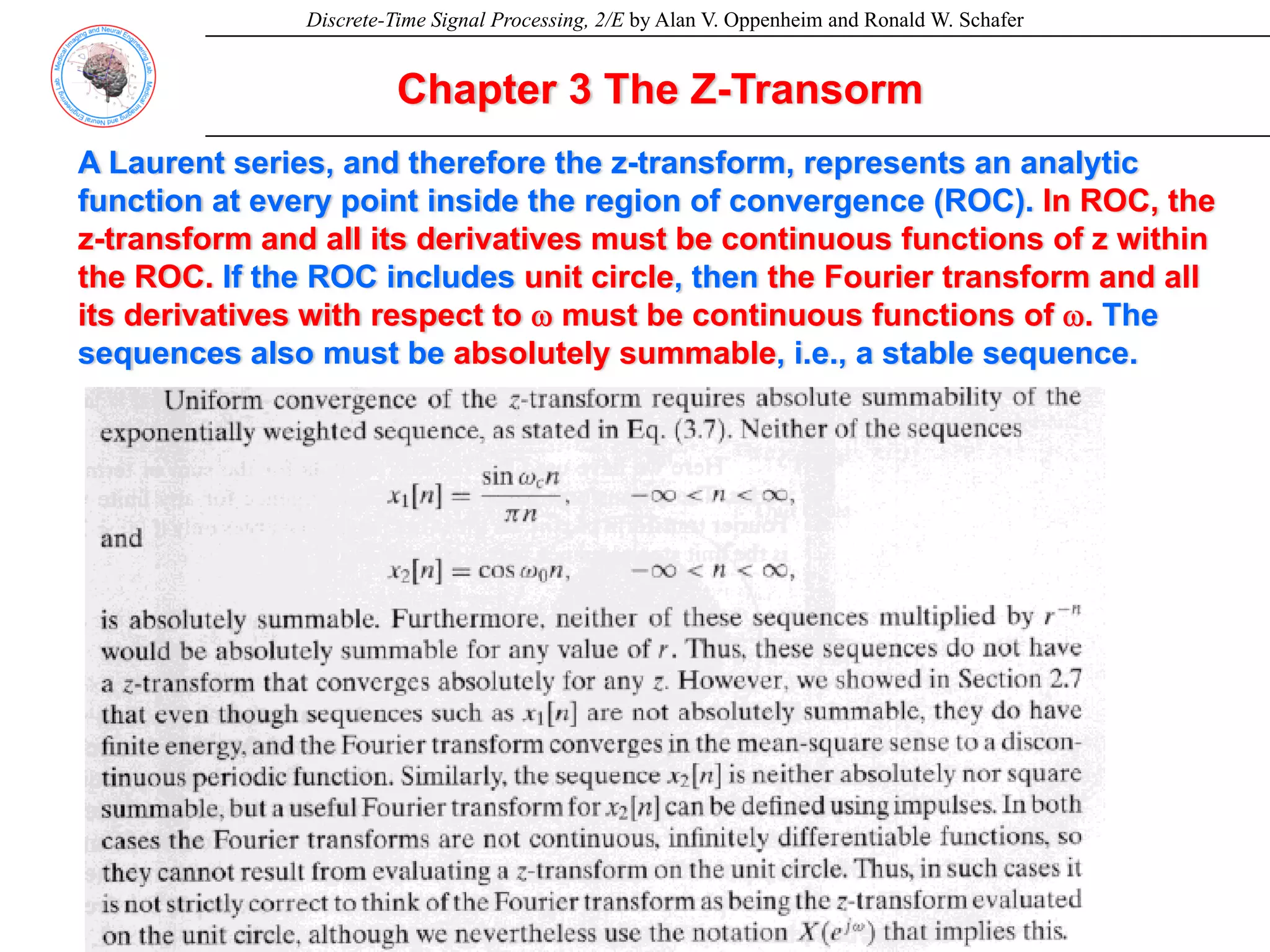
Equation (3.2) is a Laurent series.
Z-transform is a Laurent’s series
∑
∞
−∞
=
−
=
n
n
z
]
n
[
x
)
z
(
X

A Laurent series, and therefore the z-transform, represents an analytic
function at every point inside the region of convergence (ROC). In ROC, the
z-transform and all its derivatives must be continuous functions of z within
the ROC. If the ROC includes unit circle, then the Fourier transform and all
its derivatives with respect to ω must be continuous functions of ω. The
sequences also must be absolutely summable, i.e., a stable sequence.

Closed form:
Z at P(z)=0 are zeros
Z at Q(z)=0 are poles
)
z
(
Q
)
z
(
P
)
z
(
X =
Example 3.1 Right-sided Exponential Sequence
∑
∞
=
−
∞
<
0
1
n
n
|
az
|
Consider the signal x[n] = anu[n]. It is nonzero only for
n≥0, which is an example of a right-sided sequence.
∑
∑
∞
=
−
∞
−∞
=
−
=
=
0
1
n
n
n
n
n
)
az
(
z
]
n
[
u
a
)
z
(
X
Z-transform of x[n]:
For X(z) converging, it requires
|
a
|
|
z
|
a
z
z
az
)
az
(
)
z
(
X
n
n
>
−
=
−
=
= −
∞
=
−
∑ 1
0
1
1
1
1
1
1
1
>
−
= −
|
z
|
z
)
z
(
X
For a=1 , x[n] becomes unit step
sequence
.
1
1
) ω
ω
−
ω
=
−
=
<
j
j
j
e
z
given
by
ae
X(e
is
transform
Fourier
its
1,
|
a
|
For

Example 3.2 Left-sided Exponential Sequence
Consider x[n] = -anu[-n-1]. Since the sequence is nonzero for n≤ -1, it is called
left-sided sequence.
|
|
|
|
,
1
1
1
1
1
)
(
)
(
1
]
1
[
)
(
1
1
0
1
1
1
a
z
az
a
z
z
z
a
z
X
z
a
z
a
z
a
z
n
u
a
z
X
n
n
n
n
n
n
n
n
n
n
n
<
−
=
−
=
−
−
=
−
=
−
=
−
=
−
−
−
=
−
−
∞
=
−
∞
=
−
−
−∞
=
−
∞
−∞
=
−
∑
∑
∑
∑
.
1
1
) ω
ω
−
ω
=
−
=
<
j
j
j
e
z
given
by
ae
X(e
is
transform
Fourier
its
1,
|
a
|
For

Example 3.3 Sum of Two Exponential Sequences
]
[
)
3
1
(
]
[
)
2
1
(
]
[ n
u
n
u
n
x n
n
−
+
=
Consider x[n]
)
z
)(
z
(
)
z
(
z
)
z
)(
z
(
)
z
(
z
z
)
z
(
)
z
(
z
]
n
[
u
)
(
z
]
n
[
u
)
(
z
]}
n
[
u
)
(
]
n
[
u
)
{(
)
z
(
X
n
n
n
n
n
n
n
n
n
n
n
n
n
n
3
1
2
1
12
1
2
3
1
1
2
1
1
12
1
1
2
3
1
1
1
2
1
1
1
3
1
2
1
3
1
2
1
3
1
2
1
1
1
1
1
1
0
1
0
1
+
−
−
=
+
−
−
=
+
+
−
=
−
+
=
−
+
=
−
+
=
−
−
−
−
−
∞
=
−
∞
=
−
∞
−∞
=
−
∞
−∞
=
−
∞
−∞
=
−
∑
∑
∑
∑
∑
2
1
3
1
1
1
2
1
1
1
3
1
2
1
3
1
3
1
1
1
3
1
2
1
2
1
1
1
2
1
1
1
1
1
>
+
+
−
⎯→
←
−
+
>
+
⎯→
←
−
>
−
⎯→
←
−
−
−
−
|
z
|
z
z
]
n
[
u
)
(
]
n
[
u
)
(
|
z
|
z
]
n
[
u
)
(
,
|
z
|
z
]
n
[
u
)
(
Z
n
n
Z
n
Z
n

Example 3.5 Two-sided Exponential Sequence
]
n
[
u
)
(
]
n
[
u
)
(
]
n
[
x n
n
1
2
1
3
1
−
−
−
−
=
)
z
)(
z
(
)
z
(
z
)
z
)(
z
(
)
z
(
|
z
|
|,
z
|
z
z
)
z
(
X
|
z
|
z
]
n
[
u
)
(
|
z
|
z
]
n
[
u
)
(
Z
n
Z
n
2
1
3
1
12
1
2
2
1
1
3
1
1
12
1
1
2
2
1
3
1
2
1
1
1
3
1
1
1
2
1
2
1
1
1
1
2
1
3
1
3
1
1
1
3
1
1
1
1
1
1
1
1
−
+
−
=
−
+
−
=
<
<
−
+
+
=
<
−
⎯→
←
−
−
−
>
+
⎯→
←
−
−
−
−
−
−
−
Consider the Sequence

2
1
2
1
N
n
N
,
z
]
n
[
x
)
z
(
X
N
N
n
n
≤
≤
= ∑
=
−
For a sequence, x[n], with finite length, the z-transform is
It has no problem of convergence, because each of the terms |x[n]z-n| is finite.
For example ,x[n]=δ[n]+δ[n-5], then X(z)=1+z-5, which is finite for |z|>0.
The aforementioned sequences have infinite lengths, which contribute terms of the
form (1-az-1) at its denominators. It should be noticed that the term (1-az-1)
introduces both a pole and a zero.

⎩
⎨
⎧ −
≤
≤
=
otherwise
,
N
n
,
a
]
n
[
x
n
0
1
0
Example 3.6 Finite-length Sequence
a
z
a
z
z
az
)
az
(
)
az
(
z
a
)
z
(
X
N
N
N
N
N
n
n
N
n
n
n
−
−
=
−
−
=
=
=
−
−
−
−
=
−
−
=
−
∑
∑
1
1
1
1
0
1
1
0
1
1
1
Consider the signal
Then,
The ROC is determined by
1
1
0
2
1
0
1
−
=
=
∞
<
π
−
=
−
∑
N
,...,
,
k
,
ae
z
|
az
|
)
N
/
k
(
j
k
N
n
n

0
|
|
1
1
otherwise
,
0
1
0
,
.
13
|
|
]
cos
2
[
1
]
sin
[
1
]
[
]
sin
[
.
12
|
|
]
cos
2
[
1
]
cos
[
1
]
[
]
cos
[
.
11
1
|
|
]
cos
2
[
1
]
[sin
]
[
]
[sin
.
10
1
|
|
]
cos
2
[
1
]
[cos
1
]
[
]
[cos
.
9
|
|
|
|
)
1
(
]
1
[
.
8
|
|
|
|
)
1
(
]
[
.
7
|
|
|
|
1
1
]
1
[
.
6
|
|
|
|
1
1
]
[
5.
0)
m
(if
or
0)
m
(if
0
except
All
]
[
.
4
1
|
|
1
1
]
1
[
.
3
1
|
|
1
1
]
[
.
2
All
1
]
[
.
1
1
2
2
1
0
1
0
0
2
2
1
0
1
0
0
2
1
0
1
0
0
2
1
0
1
0
0
2
1
1
2
1
1
1
1
-
1
1
>
−
−
⎩
⎨
⎧ −
≤
≤
>
+
−
−
>
+
−
−
>
+
−
>
+
−
−
<
−
−
−
−
>
−
<
−
−
−
−
>
−
<
∞
>
−
<
−
−
−
−
>
−
−
−
−
−
−
−
−
−
−
−
−
−
−
−
−
−
−
−
−
−
−
−
z
az
z
a
N
n
a
r
z
z
r
z
ω
r
z
ω
r
n
u
n
ω
r
r
z
z
r
z
ω
r
z
ω
r
n
u
n
ω
r
z
z
z
ω
z
ω
n
u
n
ω
z
z
z
ω
z
ω
n
u
n
ω
a
z
az
az
n
u
na
a
z
az
az
n
u
na
a
z
az
n
u
a
a
z
az
n
u
a
z
z
m
n
z
z
n
u
z
z
n
u
z
n
N
N
n
n
n
n
n
n
n
m
σ
σ

3.2 Properties of the Region of Convergence for the z-Transform
Property 1: The ROC is a ring or disk in the z-plane centered at the origin; i.e.,
0≤rR ≤rL ≤∞.
Property 2: The Fourier transform of x[n] converges absolutely if and only if the
ROC of the z-transform of x[n] includes the unit circle.
Property 3: The ROC cannot contain any pole.
Property 4: If x[n] is a finite-duration sequence, i.e., a sequence that is zero
except in a finite interval -∞<N1 ≤n ≤N2< ∞, then the ROC is the
entire z-plane, except possibly z=0 or z= ∞.
Property 5: If x[n] is a right-sided sequence, i.e., a sequence that is nonzero for
n<N1< ∞, the ROC extends outward from the outermost (i.e., largest
magnitude) finite pole in X(z) to (and possibly including) z= ∞.
Property 6: If x[n] is a left-sided sequence, i.e., a sequence that is nonzero for
n>N2>- ∞, the ROC extends inward from the innermost (smallest
magnitude) nonzero pole in X(z) to (and possibly including) z=0;

3.2 Properties of the Region of Convergence for the z-Transform
Property 7: A two-sided sequence is an infinite-duration seqeunce that is neither
right sided nor left sided. If x[n] is a two-sided sequence, the ROC will
consist of a ring in the z-plane, bounded on the interior and exterior by
a pole and, consistent with property 3, not containing any poles.
Property 8: The ROC must be a connected region.

3.8

Example 3.8 Stability, Causality, and the ROC
Considering a system with impulse response h[n], its z-Transform H(z) has pole-
zero plot shown in Fig. 3.11. Therefore, there are three ROC possibilities.
2
1
<
|
Z
| 2
2
1
<
< |
Z
| |
Z
|
<
2
(i) (ii) (iii)
Noncausal
Not-stable
Noncausal
Stable
Causal
Not-stable
3.9 3.8

3.3 The Inverse z-Transform
3.3.1 Inspection Method
[ ] 1
1
, . (3.35)
1
z
n
a u n z a
az−
↔ >
−
1
1 1
( ) , z > (3.36)
1 2
1
2
X z
z−
⎛ ⎞
⎜ ⎟
= ⎜ ⎟
⎜ ⎟
−
⎝ ⎠
,
az
]
n
[
u
)
a
(
z
n
1
1
1
1 −
−
↔
−
−
− |
a
|
|
z
| <
,
z
)
z
(
X
⎟
⎟
⎟
⎟
⎠
⎞
⎜
⎜
⎜
⎜
⎝
⎛
−
=
−1
2
1
1
1
2
1
<
|
z
|
When use Table 3.1 to find the inverse z-transform, we should find
its ROC to find its correct z-transform.

3.3.2 Partial Fraction Expansion
0
0
( ) . (3.37)
M
k
k
k
N
k
k
k
b z
X z
a z
−
=
−
=
=
∑
∑
0
0
( ) . (3.38)
M
N M k
k
k
N
M N k
k
k
z b z
X z
z a z
−
=
−
=
=
∑
∑
1
0 1
1
0
1
(1 )
( ) . (3.39)
(1 )
M
k
k
N
k
k
c z
b
X z
a
d z
−
=
−
=
−
=
−
∏
∏
If M<N and poles are all first order
1
1
( ) . (3.40)
1
N
k
k k
A
X z
d z−
=
=
−
∑
Obviously, the common denominator of the functions in Eq. (3.42) is the
same as the denominator in Eq. (3.41). Multiplying both sides of Eq. (3.42) by
and evaluating for z=dk shows the coefficients Ak,
)
z
d
( k
1
1 −
−
1
(1 ) ( ) (3.41)
k
k k z d
A d z X z
−
=
= −
If M>N, then M-N poles at z=0, zeros at |z|=∞
If M<N, then N-M zeros at z=0, poles at |z|=∞
(3.42)
(3.41)
(3.40)
(3.43)

Example 3.9 Second-Order z-Transform
1 1
1 1
( ) , . (3.42)
1 1 2
(1 )(1 )
4 2
X z z
z z
− −
= >
− −
Consider a sequence x[n] with z-transform
Right-sided
Left or Right-sided?
)
z
(
A
)
z
(
A
)
z
(
X
1
2
1
1
2
1
1
4
1
1 −
−
−
+
−
=
1
4
1
1 4
1
1
1 −
=
−
= =
−
/
z
|
)
z
(
X
)
z
(
A 2
2
1
1 2
1
1
2 =
−
= =
−
/
z
|
)
z
(
X
)
z
(
A
)
z
(
)
z
(
)
z
(
X
1
1
2
1
1
2
4
1
1
1
−
−
−
+
−
−
=
]
n
[
u
]
n
[
u
]
n
[
x
n
n
⎟
⎠
⎞
⎜
⎝
⎛
−
⎟
⎠
⎞
⎜
⎝
⎛
=
4
1
2
1
2

0
0
( ) . (3.37)
M
k
k
k
N
k
k
k
b z
X z
a z
−
=
−
=
=
∑
∑
1
0 1
( ) . (3.43)
1
M N N
r k
r
r k k
A
X z B z
d z
−
−
−
= =
= +
−
∑ ∑
(3.42)
M ≥N
A more general form of a z-Transform X(z) with M>N contains poles at
z=0, single-order poles and multiple-order poles, which can be written as
follows,
1 1
0 1, 1
( ) . (3.44)
1 (1 )
M N N s
r k m
r m
r k k i m
k i
A C
X z B z
d z d z
−
−
− −
= = ≠ =
= + +
− −
∑ ∑ ∑
The coefficients Cm can be obtained from the equation
1
1
1
(1 ) ( ) . (3.45)
( )!( )
i
s m
s
m i
s m s m
i w d
d
C d w X w
s m d dw −
−
−
− −
=
⎧ ⎫
⎡ ⎤
= −
⎨ ⎬
⎣ ⎦
− − ⎩ ⎭
(3.39) (3.45)
(3.47)
(3.46)

[ ]
m
s
k
s
m
s
m
s
m
s
s
k
s
k
s
s
s
k
s
k
s
s
s
k
s
k
k
m
k
m
d
m
s
w
X
w
dw
d
C
C
w
d
C
w
d
C
w
X
w
Let
C
z
d
C
z
d
C
z
X
z
z
z
d
C
z
d
C
z
d
C
z
X
z
d
C
−
−
−
−
−
−
−
−
−
−
−
−
−
−
−
−
=
−
−
−
⋅
=
∴
+
+
−
⋅
+
−
⋅
=
⋅
=
+
+
−
⋅
+
−
⋅
=
⋅
−
+
+
−
+
−
=
∴
−
=
=
∑
)
(
)!
(
)
(
)
d
-
(1
)
1
(
)
1
(
)
(
)
d
-
(1
becomes
equation
the
,
z
w
)
1
(
)
1
(
)
(
)
d
-
(1
have
then we
,
)
d
-
(1
by
X(z)
Multiply
)
1
(
)
1
(
)
1
(
)
(
)
1
(
X(z)
d
at Z
poles
multiple
has
X(z)
:
example
For
1
k
2
2
1
1
1
k
1
-
2
1
2
1
1
1
1
k
1
k
1
2
1
2
1
1
s
1
m
1
k
L
L
L

Inverse Z-transform: Cauchy Integral Method
Cauchy integral formula:
∫ ≠
=
=
−
C
k
k
k
dz
z
j 0
,
0
0
,
1
{
2
1 1
π
Because
∑
∞
∞
−
−
= n
z
)
n
(
x
)
z
(
X
Multiply both sides by 1
k
z −
, then
dz
z
n
x
j
π
dz
z
z
X
j
π C
k
n
k
C
∫∑
∫
∞
∞
−
−
+
−
−
⋅
=
⋅ 1
1
)
(
2
1
)
(
2
1
∫
∑
∫
−
+
−
∞
∞
−
−
π
=
⋅
π
⇒
C
1
k
n
1
k
C
dz
z
j
2
1
)
n
(
x
dz
z
)
z
(
X
j
2
1
When –n+k=0,
)
k
(
x
dz
z
)
z
(
X
j
2
1
)
n
k
(
)
n
(
x
dz
z
)
z
(
X
j
2
1
1
k
C
1
k
C
=
⋅
π
⇒
−
δ
⋅
=
⋅
π
−
∞
∞
−
−
∫
∑
∫
Therefore, dz
z
)
z
(
X
j
)
n
(
x
n
C
1
2
1 −
∫ ⋅
π
=

Example 3.10 Inverse by Partial z-Transform
Consider a sequence x[n] with z-transform
1 2 1 2
1 2 1 1
1 2 (1 )
( ) , 1.
3 1 1
1 (1 )(1 )
2 2 2
z z z
X z z
z z z z
− − −
− − − −
+ + +
= = >
− + − −
1
2
1
2
1
1
0
1
1 −
−
−
+
−
+
=
z
A
z
A
B
)
z
(
X
Since M=2=N and all poles are all first order, X(z)
can be represented as
2
1
5
2
3
1
2
1
1
1
2
1
2
1
2
3
2
2
1
−
+
−
+
+
+
−
−
−
−
−
−
−
−
z
z
z
z
z
z
z
, where B0 =2 is found by long division
1
1 1
1 5
( ) 2 . (3.47)
1
(1 )(1 )
2
z
X z
z z
−
− −
− +
= +
− −
3.11 3.10

1
1 1
1 5
( ) 2 . (3.47)
1
(1 )(1 )
2
z
X z
z z
−
− −
− +
= +
− −
1
2
1
2
1
1
0
1
1 −
−
−
+
−
+
=
z
A
z
A
B
)
z
(
X
A1 and A2 can be calculated by residual values at z=1/2 and z=1.
9
)]
1
)(
)
1
)(
1
(
5
1
[(
)
(
)
2
1
1
(
lim
)
(
Re 2
/
1
1
2
1
1
1
2
1
1
1
2
/
1
2
/
1
−
=
−
−
−
+
−
=
−
= =
−
−
−
−
−
=
=
z
z
z
z
z
z
z
z
X
z
z
f
s
8
)]
1
)(
)
1
)(
1
(
5
1
[(
)
(
)
1
(
lim
)
(
Re 1
1
1
1
2
1
1
1
1
1
=
−
−
−
+
−
=
−
= =
−
−
−
−
−
=
=
z
z
z
z
z
z
z
z
X
z
z
f
s
1
1
9 8
( ) 2 . (3.48)
1 1
1
2
X z
z
z
−
−
= − +
−
−
Therefore,
Check Table 3.1, we get
( ) ]
n
[
u
]
n
[
u
]
n
[
]
n
[
x
n
8
9
2 2
1
+
−
δ
=

[ ]
[ ] [ ] [ ] [ ] [ ]
2 1 2
( )
2 + 1 0 1 + 2 + , (3.49)
n
n
X z x n z
x z x z x x z x z
∞
−
=−∞
− −
=
= + − − + +
∑
L L
3.3.3. Power Series Expansions
The defining expression for the z-transform is a Laurent Series where the
sequence values x[n] are the coefficients of z-n. Thus, the z-transform is
given as a power series in the form
2 1 1 1
1
( ) (1 )(1 )(1 ) (3.50)
2
X z z z z z
− − −
= − + −
Example 3.11 Finite-length Sequence
Consider
1
2
2
1
1
2
1 −
+
−
−
= z
z
z
)
z
(
X
By inspection,
]
n
[
]
n
[
]
n
[
]
n
[
]
n
[
x 1
2
1
1
2
1
2 −
δ
+
δ
−
+
δ
−
+
δ
=

Example 3.12 Inverse Transform by Power Series Expansion
Consider the z-transform
Using the Taylor series expansion for log(1+x) with |x|<1, we obtain
Therfore,
.
|
a
|
|
z
|
az
z
X >
+
= −
),
1
log(
)
( 1
.
n
z
a
z
X
n
n
n
n
∑
∞
=
−
+
−
=
1
1
)
1
(
)
(
⎪
⎩
⎪
⎨
⎧
≤
≥
−
=
+
0
n
,
1
n
,
n
a
n
x
n
n
0
)
1
(
]
[
1
1
x
1
-
for
n
x
x)
log(1
Note
n
n
n
<
<
−
=
+ ∑
∞
=
+
1
1
,
)
1
(
:
*

Example 3.13 Power Series Expansion by Long Division
1
1
( ) , > . (3.53)
1
X z z a
az−
=
−
Use Long-division, we get
Since X(z) approaches a finite
constant as z approaches infinity,
the sequences is causal.
2
2
1
2
2
2
2
1
1
1
1
1
1
1
−
−
−
−
−
−
−
+
+
−
−
−
z
a
az
z
a
z
a
az
az
az
L
+
+
+
=
−
−
−
−
2
2
1
1
1
1
1
z
a
az
az
Inverse z-
transform
]
n
[
u
a
]
n
[
x n
=
Make the long-division in descending order

Example 3.13 Power Series Expansion for a Left-sided Sequence
1
1
( ) , < . (3.54)
1
X z z a
az−
=
−
2
2
1
3
2
2
1
2
1
2
1
z
a
z
a
z
a
z
a
z
a
z
a
z
z
z
a
−
−
−
−
−
−
−
−
−
−
+
−
L
Use Long-division, we get
Since X(z) approaches a finite
constant as z approaches zero,
the sequences is causal.
]
n
[
u
a
]
n
[
x n
1
−
−
−
=
Make the long-division in ascending order

3.4 z-Transform Properties
3.4.1 Linearity
2
1
2
1
x
x
R
ROC
),
z
(
X
]
n
[
x
R
ROC
),
z
(
X
]
n
[
x
=
↔
=
↔
2
1
2
1
2
1 x
x R
R
:
ROC
),
z
(
bX
)
z
(
aX
]
n
[
bx
]
n
[
ax ∩
+
↔
+
3.4.2 Time Shifting
)
z
(
X
z
]
n
n
[
x n
z
0
0
−
↔
− , ROC=Rx (except for
the possible addition or
deletion of z=0 or z=∞)
)
z
(
X
z
z
]
m
[
x
z
z
]
n
n
[
x
z
z
]
n
n
[
x
)
z
(
Y
n
m
)
m
(
n
n
)
n
n
(
n
n
n
0
0
0
0
0
0
−
∞
−∞
=
−
−
∞
−∞
=
−
−
−
∞
−∞
=
−
=
=
−
=
−
=
∑
∑
∑

Example 3.14 Shifted Exponential Sequence
4
1
4
1
1
>
−
= |
z
|
,
z
)
z
(
X
From the ROC, we identify this as corresponding to a right-sided sequence.
( )
1
1
4
1
1 −
−
−
=
z
z
z
X ( )
1
4
1
1
4
4
−
−
+
−
=
z
z
X
( ) [ ] [ ]
n
u
n
n
x
n
⎟
⎠
⎞
⎜
⎝
⎛
+
δ
−
=
4
1
4
4
, or
( )
4
1
,
4
1
1
1
1
1
>
⎟
⎟
⎟
⎟
⎠
⎞
⎜
⎜
⎜
⎜
⎝
⎛
−
=
−
−
z
z
z
z
X [ ] [ ]
1
4
1
1
−
⎟
⎠
⎞
⎜
⎝
⎛
=
−
n
u
n
x
n

3.4.3 Multiplication by an Exponential Sequence
x
z
n
R
|
z
|
ROC
),
z
/
z
(
X
]
n
[
x
z 0
0
0 =
⎯→
←
The notation ROC=|z0|Rx denotes that ROC is Rx scaled by |z0|; i.e., if Rx is the
set of values of z such that rR<|z|<rL, then |z0|Rx is the set of values of z such that
|z0|rR<|z|<|z0|rL. This in turn can be interpreted as a frequency shift or translation,
associated with the modulation in the time domain by the complex potential
sequence ejω0n. That is
)
e
(
X
]
n
[
x
e )
(
j
z
n
j 0
0 ω
−
ω
ω
⎯→
←

Example 3.15 Exponential Multiplication
[ ] ( ) [ ]
n
u
n
r
n
x n
0
cos ω
=
]
n
[
u
)
re
(
]
n
[
u
)
re
(
]
n
[
x n
j
n
j 0
0
2
1
2
1 ω
−
ω
+
=
Calculate the z-Transform of
Rewrite is as
r
|
z
|
,
z
re
]
n
[
u
)
re
(
r
|
z
|
,
z
re
]
n
[
u
)
re
(
j
z
n
j
j
z
n
j
>
−
⎯→
←
>
−
⎯→
←
−
ω
−
ω
−
−
ω
ω
1
2
1
1
2
1
0
0
0
0
1
2
1
1
2
1
( )
( ) r
z
z
r
z
r
z
r
r
z
z
re
z
re
z
X j
j
>
+
−
−
=
>
−
+
−
=
−
−
−
−
−
−
,
cos
2
1
cos
1
,
1
2
1
1
2
1
2
2
1
0
1
0
1
1 0
0
ω
ω
ω
ω

3.4.4 Differentiation of X(z)
x
z
R
ROC
,
dz
)
z
(
dX
z
]
n
[
nx =
−
⎯→
←
∑
∞
−∞
=
−
=
n
n
z
]
n
[
x
)
z
(
X
Because
]}
n
[
nx
{
Z
z
]
n
[
nx
z
]
n
[
x
)
n
(
z
dz
)
z
(
dX
z
n
n
n
n
=
=
−
−
=
−
∑
∑
∞
−∞
=
−
∞
−∞
=
−
− 1
Consider

Example 3.16 Inverse of Non-rational z-transform
]
1
[
)
1
(
]
[
].
1
[
)
(
1
]
[
.
1
1
,
)
(
),
1
1
1
1
1
1
1
2
−
−
=
⇒
−
−
⎯
⎯→
⎯
+
⎯→
⎯
∴
+
=
⇒
+
−
=
−
⎯→
←
>
+
=
+
−
−
−
−
−
−
−
n
u
n
A
n
x
n
u
a
a
az
az
n
nx
az
az
dz
dX(z)
z
-
az
az
dz
dX(z)
then
dz
z
dX
z
nx[n]
Consider
:
Ans
.
|
a
|
|
z
|
for
az
log(1
X(z)
of
transform
-
Z
inverse
the
Find
n
n
n
z
z
z
1
-
1
-

Example 3.17 Second-Order Pole
])
n
[
u
a
(
n
]
n
[
u
na
]
n
[
x n
n
=
=
Then, we have
a
|
z
|
,
)
az
(
az
)
az
(
dz
d
z
)
z
(
X >
−
=
−
−
= −
−
− 2
1
1
1
1
1
1
2
1
1
1 )
az
(
az
]
n
[
u
na z
n
−
−
−
⎯→
←
3.4.5 Conjugation of a Complex Sequence
)
z
(
X
)
)
z
](
n
[
x
(
z
]
n
[
x
z
]
n
[
x
)
z
(
X
*
*
*
n
n
*
n
n
*
n
n
=
=
=
∑
∑
∑
∞
−∞
=
−
∞
−∞
=
−
∞
−∞
=
−
)
z
(
X
]
n
[
x
)
z
(
X
]
n
[
x
*
*
z
*
z
⎯→
←
⎯→
←
ROC=Rx

3.4.6 Time Reversal
)
z
(
X
)
)
z
](
m
[
x
(
)
)
)
z
]((
m
[
x
(
z
]
m
[
x
z
]
n
[
x
z
]
n
[
x
)
z
(
X
*
*
*
m
)
m
(
*
*
m
m
*
m
m
*
n
n
*
n
n
1
1
1
=
=
=
=
−
=
∑
∑
∑
∑
∑
∞
−∞
=
−
∞
−∞
=
−
−
∞
−∞
=
∞
−∞
=
−
∞
−∞
=
−
)
z
(
X
]
n
[
x
)
z
(
X
]
n
[
x
*
*
z
*
z
1
⎯→
←
−
⎯→
←
ROC=1/Rx
The notation ROC= 1/Rx implies that Rx is inverted; i.e., if Rx is the set of
values of z such that rR<|z|<rL, then the ROC is the set of values of z such
that 1/rL<|z|<1/rR.
)
z
(
X
)
z
](
m
[
x
)
)
z
](
m
[
x
(
z
]
m
[
x
z
]
n
[
x
z
]
n
[
x
)
z
(
X
m
m
m
m
m
m
n
n
n
n
1
1
1
=
=
=
=
−
=
∑
∑
∑
∑
∑
∞
−∞
=
−
∞
−∞
=
−
−
∞
−∞
=
∞
−∞
=
−
∞
−∞
=
−
)
z
(
X
]
n
[
x
)
z
(
X
]
n
[
x
z
z
1
⎯→
←
−
⎯→
←
ROC=1/Rx

Example 3.18 Time-Reversed Exponential Sequence
Consider
]
n
[
u
a
]
n
[
x n
−
= −
, which is a time-reversed version of anu[n]. From the time-reverse
property, it follows
1
1
1
1
1
1
1
−
−
−
−
−
−
=
−
=
z
a
z
a
az
)
z
(
X

3.4.7 Convolution of Sequence
According to the convolution property,
)
z
(
X
)
z
(
X
]
n
[
x
*
]
n
[
x z
2
1
2
1 ⎯→
←
)
z
(
X
)
z
(
X
z
}
z
]
m
[
x
]{
k
[
x
z
}
z
]
k
n
[
x
]{
k
[
x
z
]
k
n
[
x
]
k
[
x
z
}
]
k
n
[
x
]
k
[
x
{
)
z
(
Y
]
k
n
[
x
]
k
[
x
]
n
[
y
k
m
k m
k
)
k
n
(
k n
n
k n
n
n k
k
2
1
2
1
2
1
2
1
2
1
2
1
=
=
−
=
−
=
−
=
−
=
−
−
∞
−∞
=
∞
−∞
=
−
−
−
∞
−∞
=
∞
−∞
=
−
∞
−∞
=
∞
−∞
=
−
∞
−∞
=
∞
−∞
=
∞
−∞
=
∑ ∑
∑ ∑
∑ ∑
∑ ∑
∑

Example 3.19 Convolution of Finite-Length Sequence
].
3
[
]
2
[
]
1
[
]
[
]
[
.
)
(
)
(
:
].
1
[
]
[
],
2
[
]
1
[
2
]
[
−
δ
−
−
δ
−
−
δ
+
δ
=
⇒
+
=
⋅
+
+
=
=
∴
=
+
+
=
−
δ
−
δ
=
−
δ
+
−
δ
+
δ
=
n
n
n
n
n
y
z
-
z
-
z
1
z
-
1
z
2z
1
X2(z)
X1(z)
Y(z)
z
-
1
X2(z)
and
z
2z
1
X1(z)
Answer
n
n
x2[n]
and
n
n
n
x1[n]
which
in
[n],
x
and
[n]
x
sequences
length
-
finite
two
of
y[n]
n
convolutio
the
find
Please
3
-
2
-
1
-
1
-
2
-
1
-
1
-
2
-
1
-
2
1

3.4.10 Initial Value Theorem
If x[n] is zero for n<0 (i.e., if x[n] is causal), then
]
[
x
|
z
]
n
[
x
|
z
]
n
[
x
|
)
z
(
X
)
z
(
X
lim
]
[
x
z
n
n
z
n
n
z
z
0
0
0
=
=
=
=
∞
→
∞
=
−
∞
→
∞
−∞
=
−
∞
→
∞
→
∑
∑
causal

3.5 z-Transforms and LTI systems
Example 3.20 Evaluating a Convolution Using the z-Transform
Let h[n]=anu[n] and x[n]=Au[n]. The corresponding z-Transforms are
1
|
|
,
)
1
)(
(
)
1
)(
1
(
)
(
)
(
)
(
1
|
|
,
1
)
(
|
|
|
|
,
1
1
)
(
2
1
1
2
1
1
0
1
0
>
−
−
=
−
−
=
=
>
−
=
=
>
−
=
=
−
−
−
∞
=
−
−
∞
=
−
∑
∑
z
z
a
z
Az
z
az
A
z
X
z
X
z
Y
z
z
A
Az
z
X
a
z
az
z
a
z
H
n
n
n
n
n
If |a|<1, then the z-transform of the convolution of h[n] and x[n] is

Ch3_Z-transform.pdf

More Related Content

Similar to Ch3_Z-transform.pdf

More from shannlevia123

Recently uploaded

Ch3_Z-transform.pdf