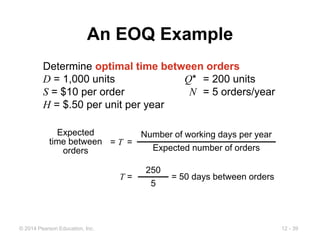
12 - 1
© 2014 Pearson Education, Inc.
Inventory
Management
PowerPoint presentation to accompany
Heizer and Render
Operations Management, Eleventh Edition
Principles of Operations Management, Ninth Edition
PowerPoint slides by Jeff Heyl
12
© 2014 Pearson Education, Inc.
12 - 2
© 2014 Pearson Education, Inc.
Outline
► Global Company Profile:
Amazon.com
► The Importance of Inventory
► Managing Inventory
► Inventory Models
► Inventory Models for Independent
Demand
12 - 3
© 2014 Pearson Education, Inc.
Outline - Continued
► Probabilistic Models and
Safety Stock
► Single-Period Model
► Fixed-Period (P) Systems
12 - 4
© 2014 Pearson Education, Inc.
Learning Objectives
When you complete this chapter you
should be able to:
1. Conduct an ABC analysis
2. Explain and use cycle counting
3. Explain and use the EOQ model for
independent inventory demand
4. Compute a reorder point and safety
stock
12 - 5
© 2014 Pearson Education, Inc.
Learning Objectives
When you complete this chapter you
should be able to:
5. Apply the production order quantity
model
6. Explain and use the quantity discount
model
7. Understand service levels and
probabilistic inventory models
12 - 6
© 2014 Pearson Education, Inc.
Inventory Management at
Amazon.com
► Amazon.com started as a “virtual”
retailer – no inventory, no warehouses,
no overhead; just computers taking
orders to be filled by others
► Growth has forced Amazon.com to
become a world leader in warehousing
and inventory management
© 2014 Pearson Education, Inc.
12 - 7
© 2014 Pearson Education, Inc.
Inventory Management at
Amazon.com
1.Each order is assigned by computer to the
closest distribution center that has the
product(s)
2.A “flow meister” at each distribution center
assigns work crews
3.Lights indicate products that are to be picked
and the light is reset
4.Items are placed in crates on a conveyor, bar
code scanners scan each item 15 times to
virtually eliminate errors
© 2014 Pearson Education, Inc.
12 - 8
© 2014 Pearson Education, Inc.
Inventory Management at
Amazon.com
5. Crates arrive at central point where items
are boxed and labeled with new bar code
6. Gift wrapping is done by hand at 30
packages per hour
7. Completed boxes are packed, taped,
weighed and labeled before leaving
warehouse in a truck
8. Order arrives at customer within 1 - 2 days
© 2014 Pearson Education, Inc.
12 - 9
© 2014 Pearson Education, Inc.
Inventory Management
The objective of inventory
management is to strike a balance
between inventory investment and
customer service
12 - 10
© 2014 Pearson Education, Inc.
Importance of Inventory
▶One of the most expensive assets of
many companies representing as
much as 50% of total invested capital
▶Operations managers must balance
inventory investment and customer
service
12 - 11
© 2014 Pearson Education, Inc.
Functions of Inventory
1. To provide a selection of goods for
anticipated demand and to separate
the firm from fluctuations in demand
2. To decouple or separate various
parts of the production process
3. To take advantage of quantity
discounts
4. To hedge against inflation
12 - 12
© 2014 Pearson Education, Inc.
Types of Inventory
▶Raw material
▶Purchased but not processed
▶Work-in-process (WIP)
▶Undergone some change but not completed
▶A function of cycle time for a product
▶Maintenance/repair/operating (MRO)
▶Necessary to keep machinery and processes
productive
▶Finished goods
▶Completed product awaiting shipment
12 - 13
© 2014 Pearson Education, Inc.
The Material Flow Cycle
Figure 12.1
Input Wait for Wait to Move Wait in queue Setup Run Output
inspection be moved time for operator time time
Cycle time
95% 5%
12 - 14
© 2014 Pearson Education, Inc.
Managing Inventory
1. How inventory items can be classified
(ABC analysis)
2. How accurate inventory records can
be maintained
12 - 15
© 2014 Pearson Education, Inc.
ABC Analysis
▶Divides inventory into three classes based
on annual dollar volume
▶Class A - high annual dollar volume
▶Class B - medium annual dollar volume
▶Class C - low annual dollar volume
▶Used to establish policies that focus on the
few critical parts and not the many trivial
ones
12 - 16
© 2014 Pearson Education, Inc.
ABC Analysis
ABC Calculation
(1) (2) (3) (4) (5) (6) (7)
ITEM
STOCK
NUMBER
PERCENT
OF
NUMBER
OF ITEMS
STOCKED
ANNUAL
VOLUME
(UNITS) x
UNIT
COST =
ANNUAL
DOLLAR
VOLUME
PERCENT
OF ANNUAL
DOLLAR
VOLUME CLASS
#10286 20% 1,000 $ 90.00 $ 90,000 38.8% A
#11526 500 154.00 77,000 33.2% A
#12760 1,550 17.00 26,350 11.3% B
#10867 30% 350 42.86 15,001 6.4% B
#10500 1,000 12.50 12,500 5.4% B
#12572 600 $ 14.17 $ 8,502 3.7% C
#14075 2,000 .60 1,200 .5% C
#01036 50% 100 8.50 850 .4% C
#01307 1,200 .42 504 .2% C
#10572 250 .60 150 .1% C
8,550 $232,057 100.0%
72%
23%
5%
12 - 17
© 2014 Pearson Education, Inc.
ABC Analysis
A Items
B Items
| | | | | | | | | |
10 20 30 40 50 60 70 80 90 100
Percentage
of
annual
dollar
usage
80 –
70 –
60 –
50 –
40 –
30 –
20 –
10 –
0 –
Percentage of inventory items
Figure 12.2
C Items
12 - 18
© 2014 Pearson Education, Inc.
ABC Analysis
▶ Other criteria than annual dollar volume
may be used
▶ High shortage or holding cost
▶ Anticipated engineering changes
▶ Delivery problems
▶ Quality problems
12 - 19
© 2014 Pearson Education, Inc.
ABC Analysis
▶Policies employed may include
1. More emphasis on supplier development for
A items
2. Tighter physical inventory control for A items
3. More care in forecasting A items
12 - 20
© 2014 Pearson Education, Inc.
Record Accuracy
► Accurate records are a critical
ingredient in production and
inventory systems
► Periodic systems require regular
checks of inventory
► Two-bin system
► Perpetual inventory tracks receipts
and subtractions on a continuing basis
► May be semi-automated
12 - 21
© 2014 Pearson Education, Inc.
Record Accuracy
► Incoming and outgoing
record keeping must be
accurate
► Stockrooms should be secure
► Necessary to make precise decisions
about ordering, scheduling, and
shipping
12 - 22
© 2014 Pearson Education, Inc.
Cycle Counting
▶Items are counted and records updated on
a periodic basis
▶Often used with ABC analysis
▶Has several advantages
1. Eliminates shutdowns and interruptions
2. Eliminates annual inventory adjustment
3. Trained personnel audit inventory accuracy
4. Allows causes of errors to be identified and
corrected
5. Maintains accurate inventory records
12 - 23
© 2014 Pearson Education, Inc.
Cycle Counting Example
5,000 items in inventory, 500 A items, 1,750 B items, 2,750 C
items
Policy is to count A items every month (20 working days), B items
every quarter (60 days), and C items every six months (120 days)
ITEM
CLASS QUANTITY
CYCLE
COUNTING
POLICY
NUMBER OF ITEMS
COUNTED PER DAY
A 500 Each month 500/20 = 25/day
B 1,750 Each quarter 1,750/60 = 29/day
C 2,750 Every 6 months 2,750/120 = 23/day
77/day
12 - 24
© 2014 Pearson Education, Inc.
Control of Service Inventories
▶Can be a critical component
of profitability
▶Losses may come from
shrinkage or pilferage
▶Applicable techniques include
1. Good personnel selection, training, and
discipline
2. Tight control of incoming shipments
3. Effective control of all goods leaving facility
12 - 25
© 2014 Pearson Education, Inc.
Inventory Models
▶Independent demand - the demand for
item is independent of the demand for any
other item in inventory
▶Dependent demand - the demand for
item is dependent upon the demand for
some other item in the inventory
12 - 26
© 2014 Pearson Education, Inc.
Inventory Models
▶Holding costs - the costs of holding or
“carrying” inventory over time
▶Ordering costs - the costs of placing an
order and receiving goods
▶Setup costs - cost to prepare a machine
or process for manufacturing an order
▶May be highly correlated with setup time
12 - 27
© 2014 Pearson Education, Inc.
Holding Costs
TABLE 12.1 Determining Inventory Holding Costs
CATEGORY
COST (AND RANGE)
AS A PERCENT OF
INVENTORY VALUE
Housing costs (building rent or depreciation,
operating costs, taxes, insurance)
6% (3 - 10%)
Material handling costs (equipment lease or
depreciation, power, operating cost)
3% (1 - 3.5%)
Labor cost (receiving, warehousing, security) 3% (3 - 5%)
Investment costs (borrowing costs, taxes, and
insurance on inventory)
11% (6 - 24%)
Pilferage, space, and obsolescence (much
higher in industries undergoing rapid change like
PCs and cell phones)
3% (2 - 5%)
Overall carrying cost 26%
12 - 28
© 2014 Pearson Education, Inc.
Holding Costs
TABLE 12.1 Determining Inventory Holding Costs
CATEGORY
COST (AND RANGE)
AS A PERCENT OF
INVENTORY VALUE
Housing costs (building rent or depreciation,
operating costs, taxes, insurance)
6% (3 - 10%)
Material handling costs (equipment lease or
depreciation, power, operating cost)
3% (1 - 3.5%)
Labor cost (receiving, warehousing, security) 3% (3 - 5%)
Investment costs (borrowing costs, taxes, and
insurance on inventory)
11% (6 - 24%)
Pilferage, space, and obsolescence (much
higher in industries undergoing rapid change like
PCs and cell phones)
3% (2 - 5%)
Overall carrying cost 26%
12 - 29
© 2014 Pearson Education, Inc.
Inventory Models for
Independent Demand
Need to determine when and
how much to order
1. Basic economic order quantity
(EOQ) model
2. Production order quantity model
3. Quantity discount model
12 - 30
© 2014 Pearson Education, Inc.
Basic EOQ Model
1. Demand is known, constant, and independent
2. Lead time is known and constant
3. Receipt of inventory is instantaneous and
complete
4. Quantity discounts are not possible
5. Only variable costs are setup (or ordering)
and holding
6. Stockouts can be completely avoided
Important assumptions
12 - 31
© 2014 Pearson Education, Inc.
Inventory Usage Over Time
Figure 12.3
Order
quantity = Q
(maximum
inventory
level)
Usage rate
Average
inventory
on hand
Q
2
Minimum
inventory
Inventory
level
Time
0
Total order received
12 - 32
© 2014 Pearson Education, Inc.
Minimizing Costs
Objective is to minimize total costs
Table 12.4(c)
Annual
cost
Order quantity
Total cost of
holding and
setup (order)
Holding cost
Setup (order) cost
Minimum
total cost
Optimal order
quantity (Q*)
12 - 33
© 2014 Pearson Education, Inc.
Minimizing Costs
▶By minimizing the sum of setup (or
ordering) and holding costs, total costs are
minimized
▶Optimal order size Q* will minimize total
cost
▶A reduction in either cost reduces the total
cost
▶Optimal order quantity occurs when
holding cost and setup cost are equal
12 - 34
© 2014 Pearson Education, Inc.
Minimizing Costs
Q = Number of pieces per order
Q* = Optimal number of pieces per order (EOQ)
D = Annual demand in units for the inventory item
S = Setup or ordering cost for each order
H = Holding or carrying cost per unit per year
Annual setup cost = (Number of orders placed per year)
x (Setup or order cost per order)
Annual demand
Number of units in each order
Setup or order
cost per order
=
=
D
Q
æ
è
ç
ö
ø
÷S
Annual setup cost =
D
Q
S
12 - 35
© 2014 Pearson Education, Inc.
Q = Number of pieces per order
Q* = Optimal number of pieces per order (EOQ)
D = Annual demand in units for the inventory item
S = Setup or ordering cost for each order
H = Holding or carrying cost per unit per year
Minimizing Costs
Annual holding cost = (Average inventory level)
x (Holding cost per unit per year)
Order quantity
2
(Holding cost per unit per year)
=
=
Q
2
æ
è
ç
ö
ø
÷H
Annual setup cost =
D
Q
S
Annual holding cost =
Q
2
H
12 - 36
© 2014 Pearson Education, Inc.
Minimizing Costs
D
Q
S =
Q
2
æ
è
ç
ö
ø
÷H
Optimal order quantity is found when annual setup
cost equals annual holding cost
Solving for Q* 2DS = Q2
H
Q2
=
2DS
H
Q*
=
2DS
H
Q = Number of pieces per order
Q* = Optimal number of pieces per order (EOQ)
D = Annual demand in units for the inventory item
S = Setup or ordering cost for each order
H = Holding or carrying cost per unit per year
Annual setup cost =
D
Q
S
Annual holding cost =
Q
2
H
12 - 37
© 2014 Pearson Education, Inc.
An EOQ Example
Determine optimal number of needles to order
D = 1,000 units
S = $10 per order
H = $.50 per unit per year
Q*
=
2DS
H
Q*
=
2(1,000)(10)
0.50
= 40,000 = 200 units
12 - 38
© 2014 Pearson Education, Inc.
An EOQ Example
Determine expected number of orders
D = 1,000 units Q* = 200 units
S = $10 per order
H = $.50 per unit per year
N = = 5 orders per year
1,000
200
= N = =
Expected
number of
orders
Demand
Order quantity
D
Q*
12 - 39
© 2014 Pearson Education, Inc.
An EOQ Example
Determine optimal time between orders
D = 1,000 units Q* = 200 units
S = $10 per order N = 5 orders/year
H = $.50 per unit per year
T = = 50 days between orders
250
5
= T =
Expected
time between
orders
Number of working days per year
Expected number of orders
12 - 40
© 2014 Pearson Education, Inc.
An EOQ Example
Determine the total annual cost
D = 1,000 units Q* = 200 units
S = $10 per order N = 5 orders/year
H = $.50 per unit per year T = 50 days
Total annual cost = Setup cost + Holding cost
TC =
D
Q
S +
Q
2
H
=
1,000
200
($10)+
200
2
($.50)
= (5)($10)+(100)($.50)
= $50+$50 = $100
12 - 41
© 2014 Pearson Education, Inc.
The EOQ Model
When including actual cost of material P
Total annual cost = Setup cost + Holding cost + Product cost
TC =
D
Q
S +
Q
2
H + PD
12 - 42
© 2014 Pearson Education, Inc.
Robust Model
▶The EOQ model is robust
▶It works even if all parameters and
assumptions are not met
▶The total cost curve is relatively flat in
the area of the EOQ
12 - 43
© 2014 Pearson Education, Inc.
An EOQ Example
Determine optimal number of needles to order
D = 1,000 units Q* = 200 units
S = $10 per order N = 5 orders/year
H = $.50 per unit per year T = 50 days
TC =
D
Q
S +
Q
2
H
=
1,500
200
($10)+
200
2
($.50)
= $75+$50 = $125
1,500 units
=
1,500
244.9
($10)+
244.9
2
($.50)
= 6.125($10)+122.45($.50)
= $61.25+$61.22 = $122.47
Only 2% less than
the total cost of
$125 when the
order quantity was
200
12 - 44
© 2014 Pearson Education, Inc.
Reorder Points
▶ EOQ answers the “how much” question
▶ The reorder point (ROP) tells “when” to order
▶ Lead time (L) is the time between placing and
receiving an order
ROP =
Lead time for a new
order in days
Demand
per day
= d x L
d =
D
Number of working days in a year
12 - 45
© 2014 Pearson Education, Inc.
Reorder Point Curve
Q*
ROP
(units)
Inventory
level
(units)
Time (days)
Figure 12.5
Lead time = L
Slope = units/day = d
Resupply takes place as order arrives
12 - 46
© 2014 Pearson Education, Inc.
Reorder Point Example
Demand = 8,000 iPods per year
250 working day year
Lead time for orders is 3 working days, may take 4
ROP = d x L
d =
D
Number of working days in a year
= 8,000/250 = 32 units
= 32 units per day x 3 days = 96 units
= 32 units per day x 4 days = 128 units
12 - 47
© 2014 Pearson Education, Inc.
Production Order Quantity Model
1. Used when inventory builds up over a
period of time after an order is placed
2. Used when units are produced and
sold simultaneously
Inventory
level
Time
Demand part of cycle with
no production (only usage)
Part of inventory cycle during which
production (and usage) is taking place
t
Maximum
inventory
Figure 12.6
12 - 48
© 2014 Pearson Education, Inc.
Production Order Quantity Model
Q = Number of pieces per order p = Daily production rate
H = Holding cost per unit per year d = Daily demand/usage rate
t = Length of the production run in days
= (Average inventory level) x
Annual inventory
holding cost
Holding cost
per unit per year
= (Maximum inventory level)/2
Annual inventory
level
= –
Maximum
inventory level
Total produced during
the production run
Total used during
the production run
= pt – dt
12 - 49
© 2014 Pearson Education, Inc.
Production Order Quantity Model
Q = Number of pieces per order p = Daily production rate
H = Holding cost per unit per year d = Daily demand/usage rate
t = Length of the production run in days
= –
Maximum
inventory level
Total produced during
the production run
Total used during
the production run
= pt – dt
However, Q = total produced = pt ; thus t = Q/p
Maximum
inventory level = p – d = Q 1 –
Q
p
Q
p
d
p
Holding cost = (H) = 1 – H
d
p
Q
2
Maximum inventory level
2
12 - 50
© 2014 Pearson Education, Inc.
Production Order Quantity Model
Q = Number of pieces per order p = Daily production rate
H = Holding cost per unit per year d = Daily demand/usage rate
t = Length of the production run in days
Setup cost = (D / Q)S
Holding cost = 1
2
HQ 1- d p
( )
é
ë
ù
û
D
Q
S = 1
2
HQ 1- d p
( )
é
ë
ù
û
Q2
=
2DS
H 1- d p
( )
é
ë
ù
û
Qp
*
=
2DS
H 1- d p
( )
é
ë
ù
û
12 - 51
© 2014 Pearson Education, Inc.
Production Order Quantity
Example
D = 1,000 units p = 8 units per day
S = $10 d = 4 units per day
H = $0.50 per unit per year
Qp
*
=
2DS
H 1- d p
( )
é
ë
ù
û
Qp
*
=
2(1,000)(10)
0.50 1-(4 8)
é
ë
ù
û
=
20,000
0.50(1 2)
= 80,000
= 282.8 hubcaps, or 283 hubcaps
12 - 52
© 2014 Pearson Education, Inc.
Production Order Quantity Model
When annual data are used the equation becomes
Note:
d = 4 = =
D
Number of days the plant is in operation
1,000
250
Qp
*
=
2DS
H 1-
Annual demand rate
Annual production rate
æ
è
ç
ö
ø
÷
12 - 53
© 2014 Pearson Education, Inc.
Quantity Discount Models
▶Reduced prices are often available when larger
quantities are purchased
▶Trade-off is between reduced product cost and
increased holding cost
TABLE 12.2 A Quantity Discount Schedule
DISCOUNT
NUMBER DISCOUNT QUANTITY DISCOUNT (%)
DISCOUNT
PRICE (P)
1 0 to 999 no discount $5.00
2 1,000 to 1,999 4 $4.80
3 2,000 and over 5 $4.75
12 - 54
© 2014 Pearson Education, Inc.
Quantity Discount Models
Q*
=
2DS
IP
Total annual cost = Setup cost + Holding cost + Product cost
TC =
D
Q
S +
Q
2
H + PD
where Q = Quantity ordered P = Price per unit
D = Annual demand in units H = Holding cost per unit per year
S = Ordering or setup cost per order
Because unit price varies, holding cost (H) is
expressed as a percent (I) of unit price (P)
12 - 55
© 2014 Pearson Education, Inc.
Quantity Discount Models
Steps in analyzing a quantity discount
1. For each discount, calculate Q*
2. If Q* for a discount doesn’t qualify, choose
the lowest possible quantity to get the
discount
3. Compute the total cost for each Q* or
adjusted value from Step 2
4. Select the Q* that gives the lowest total
cost
12 - 56
© 2014 Pearson Education, Inc.
Quantity Discount Models
1,000 2,000
Total
cost
$
0
Order quantity
Q* for discount 2 is below the allowable range at point a and
must be adjusted upward to 1,000 units at point b
a
b
1st price
break
2nd price
break
Total cost
curve for
discount 1
Total cost curve for discount 2
Total cost curve for discount 3
Figure 12.7
12 - 57
© 2014 Pearson Education, Inc.
Quantity Discount Example
Calculate Q* for every discount
Q1* = = 700 cars/order
2(5,000)(49)
(.2)(5.00)
Q2* = = 714 cars/order
2(5,000)(49)
(.2)(4.80)
Q3* = = 718 cars/order
2(5,000)(49)
(.2)(4.75)
Q*
=
2DS
IP
12 - 58
© 2014 Pearson Education, Inc.
Quantity Discount Example
Calculate Q* for every discount
Q1* = = 700 cars/order
2(5,000)(49)
(.2)(5.00)
Q2* = = 714 cars/order
2(5,000)(49)
(.2)(4.80)
Q3* = = 718 cars/order
2(5,000)(49)
(.2)(4.75)
Q*
=
2DS
IP
1,000 — adjusted
2,000 — adjusted
12 - 59
© 2014 Pearson Education, Inc.
Quantity Discount Example
TABLE 12.3 Total Cost Computations for Wohl’s Discount Store
DISCOUNT
NUMBER
UNIT
PRICE
ORDER
QUANTITY
ANNUAL
PRODUCT
COST
ANNUAL
ORDERING
COST
ANNUAL
HOLDING
COST TOTAL
1 $5.00 700 $25,000 $350 $350 $25,700
2 $4.80 1,000 $24,000 $245 $480 $24,725
3 $4.75 2,000 $23.750 $122.50 $950 $24,822.50
Choose the price and quantity that gives the
lowest total cost
Buy 1,000 units at $4.80 per unit
12 - 60
© 2014 Pearson Education, Inc.
Probabilistic Models and
Safety Stock
▶Used when demand is not constant or certain
▶Use safety stock to achieve a desired service
level and avoid stockouts
ROP = d x L + ss
Annual stockout costs = the sum of the units short x
the probability x the stockout cost/unit
x the number of orders per year
12 - 61
© 2014 Pearson Education, Inc.
Safety Stock Example
NUMBER OF UNITS PROBABILITY
30 .2
40 .2
ROP  50 .3
60 .2
70 .1
1.0
ROP = 50 units Stockout cost = $40 per frame
Orders per year = 6 Carrying cost = $5 per frame per year
12 - 62
© 2014 Pearson Education, Inc.
Safety Stock Example
ROP = 50 units Stockout cost = $40 per frame
Orders per year = 6 Carrying cost = $5 per frame per year
SAFETY
STOCK
ADDITIONAL
HOLDING COST STOCKOUT COST
TOTAL
COST
20 (20)($5) = $100 $0 $100
10 (10)($5) = $ 50 (10)(.1)($40)(6) = $240 $290
0 $ 0 (10)(.2)($40)(6) + (20)(.1)($40)(6) = $960 $960
A safety stock of 20 frames gives the lowest total cost
ROP = 50 + 20 = 70 frames
12 - 63
© 2014 Pearson Education, Inc.
Safety stock 16.5 units
ROP 
Place
order
Probabilistic Demand
Inventory
level
Time
0
Minimum demand during lead time
Maximum demand during lead time
Mean demand during lead time
Normal distribution probability of
demand during lead time
Expected demand during lead time (350 kits)
ROP = 350 + safety stock of 16.5 = 366.5
Receive
order
Lead
time
Figure 12.8
12 - 64
© 2014 Pearson Education, Inc.
Probabilistic Demand
Use prescribed service levels to set safety
stock when the cost of stockouts cannot be
determined
ROP = demand during lead time + ZsdLT
where Z = Number of standard deviations
sdLT = Standard deviation of demand during lead
time
12 - 65
© 2014 Pearson Education, Inc.
Probabilistic Demand
Safety
stock
Probability of
no stockout
95% of the time
Mean
demand
350
ROP = ? kits Quantity
Number of
standard deviations
0 z
Risk of a stockout
(5% of area of
normal curve)
12 - 66
© 2014 Pearson Education, Inc.
Probabilistic Example
m = Average demand = 350 kits
sdLT = Standard deviation of
demand during lead time = 10 kits
Z = 5% stockout policy (service level = 95%)
Using Appendix I, for an area under the curve of
95%, the Z = 1.65
Safety stock = ZsdLT = 1.65(10) = 16.5 kits
Reorder point = Expected demand during lead time +
Safety stock
= 350 kits + 16.5 kits of safety stock
= 366.5 or 367 kits
12 - 67
© 2014 Pearson Education, Inc.
Other Probabilistic Models
▶When data on demand during lead time is
not available, there are other models
available
1. When demand is variable and lead time is
constant
2. When lead time is variable and demand is
constant
3. When both demand and lead time are
variable
12 - 68
© 2014 Pearson Education, Inc.
Other Probabilistic Models
Demand is variable and lead time is constant
ROP = (Average daily demand
x Lead time in days) + ZsdLT
where sdLT = sd Lead time
sd = standard deviation of demand per day
12 - 69
© 2014 Pearson Education, Inc.
Probabilistic Example
Average daily demand (normally distributed) = 15
Lead time in days (constant) = 2
Standard deviation of daily demand = 5
Service level = 90%
Z for 90% = 1.28
From Appendix I
ROP = (15 units x 2 days) + ZsdLT
= 30 + 1.28(5)( 2)
= 30 + 9.02 = 39.02 ≈ 39
Safety stock is about 9 computers
12 - 70
© 2014 Pearson Education, Inc.
Other Probabilistic Models
Lead time is variable and demand is constant
ROP = (Daily demand x Average lead
time in days) + Z x (Daily
demand) x sLT
where sLT = Standard deviation of lead time in days
12 - 71
© 2014 Pearson Education, Inc.
Probabilistic Example
Daily demand (constant) = 10
Average lead time = 6 days
Standard deviation of lead time = sLT = 1
Service level = 98%, so Z (from Appendix I) = 2.055
ROP = (10 units x 6 days) + 2.055(10 units)(1)
= 60 + 20.55 = 80.55
Reorder point is about 81 cameras
12 - 72
© 2014 Pearson Education, Inc.
Other Probabilistic Models
Both demand and lead time are variable
ROP = (Average daily demand
x Average lead time) + ZsdLT
where sd = Standard deviation of demand per day
sLT = Standard deviation of lead time in days
sdLT = (Average lead time x sd
2)
+ (Average daily demand)2s2
LT
12 - 73
© 2014 Pearson Education, Inc.
Probabilistic Example
Average daily demand (normally distributed) = 150
Standard deviation = sd = 16
Average lead time 5 days (normally distributed)
Standard deviation = sLT = 1 day
Service level = 95%, so Z = 1.65 (from Appendix I)
ROP = (150 packs´5 days)+1.65sdLT
sdLT
= 5 days´162
( )+ 1502
´12
( ) = 5´256
( )+ 22,500´1
( )
= 1,280
( )+ 22,500
( ) = 23,780 @154
ROP = (150´5)+1.65(154) @ 750+254 =1,004 packs
12 - 74
© 2014 Pearson Education, Inc.
Single-Period Model
▶Only one order is placed for a product
▶Units have little or no value at the end of the
sales period
Cs = Cost of shortage = Sales price/unit – Cost/unit
Co = Cost of overage = Cost/unit – Salvage value
Service level =
Cs
Cs + Co
12 - 75
© 2014 Pearson Education, Inc.
Single-Period Example
Average demand = m = 120 papers/day
Standard deviation = s = 15 papers
Cs = cost of shortage = $1.25 – $.70 = $.55
Co = cost of overage = $.70 – $.30 = $.40
Service level =
Cs
Cs + Co
=
= = .579
.55
.55 + .40
.55
.95
Service
level
57.9%
Optimal stocking level
m = 120
12 - 76
© 2014 Pearson Education, Inc.
Single-Period Example
From Appendix I, for the area .579, Z  .20
The optimal stocking level
= 120 copies + (.20)(s)
= 120 + (.20)(15) = 120 + 3 = 123 papers
The stockout risk = 1 – Service level
= 1 – .579 = .422 = 42.2%
12 - 77
© 2014 Pearson Education, Inc.
Fixed-Period (P) Systems
▶Orders placed at the end of a fixed
period
▶Inventory counted only at end of period
▶Order brings inventory up to target level
▶Only relevant costs are ordering and
holding
▶Lead times are known and constant
▶Items are independent of one another
12 - 78
© 2014 Pearson Education, Inc.
Fixed-Period (P) Systems
On-hand
inventory
Time
Q1
Q2
Target quantity (T)
P
Q3
Q4
P
P
Figure 12.9
12 - 79
© 2014 Pearson Education, Inc.
Fixed-Period Systems
▶Inventory is only counted at each
review period
▶May be scheduled at convenient times
▶Appropriate in routine situations
▶May result in stockouts between
periods
▶May require increased safety stock
12 - 80
© 2014 Pearson Education, Inc.
All rights reserved. No part of this publication may be reproduced, stored in a retrieval system, or
transmitted, in any form or by any means, electronic, mechanical, photocopying, recording, or
otherwise, without the prior written permission of the publisher.
Printed in the United States of America.

Inventory.pptx

  • 1.
    12 - 1 ©2014 Pearson Education, Inc. Inventory Management PowerPoint presentation to accompany Heizer and Render Operations Management, Eleventh Edition Principles of Operations Management, Ninth Edition PowerPoint slides by Jeff Heyl 12 © 2014 Pearson Education, Inc.
  • 2.
    12 - 2 ©2014 Pearson Education, Inc. Outline ► Global Company Profile: Amazon.com ► The Importance of Inventory ► Managing Inventory ► Inventory Models ► Inventory Models for Independent Demand
  • 3.
    12 - 3 ©2014 Pearson Education, Inc. Outline - Continued ► Probabilistic Models and Safety Stock ► Single-Period Model ► Fixed-Period (P) Systems
  • 4.
    12 - 4 ©2014 Pearson Education, Inc. Learning Objectives When you complete this chapter you should be able to: 1. Conduct an ABC analysis 2. Explain and use cycle counting 3. Explain and use the EOQ model for independent inventory demand 4. Compute a reorder point and safety stock
  • 5.
    12 - 5 ©2014 Pearson Education, Inc. Learning Objectives When you complete this chapter you should be able to: 5. Apply the production order quantity model 6. Explain and use the quantity discount model 7. Understand service levels and probabilistic inventory models
  • 6.
    12 - 6 ©2014 Pearson Education, Inc. Inventory Management at Amazon.com ► Amazon.com started as a “virtual” retailer – no inventory, no warehouses, no overhead; just computers taking orders to be filled by others ► Growth has forced Amazon.com to become a world leader in warehousing and inventory management © 2014 Pearson Education, Inc.
  • 7.
    12 - 7 ©2014 Pearson Education, Inc. Inventory Management at Amazon.com 1.Each order is assigned by computer to the closest distribution center that has the product(s) 2.A “flow meister” at each distribution center assigns work crews 3.Lights indicate products that are to be picked and the light is reset 4.Items are placed in crates on a conveyor, bar code scanners scan each item 15 times to virtually eliminate errors © 2014 Pearson Education, Inc.
  • 8.
    12 - 8 ©2014 Pearson Education, Inc. Inventory Management at Amazon.com 5. Crates arrive at central point where items are boxed and labeled with new bar code 6. Gift wrapping is done by hand at 30 packages per hour 7. Completed boxes are packed, taped, weighed and labeled before leaving warehouse in a truck 8. Order arrives at customer within 1 - 2 days © 2014 Pearson Education, Inc.
  • 9.
    12 - 9 ©2014 Pearson Education, Inc. Inventory Management The objective of inventory management is to strike a balance between inventory investment and customer service
  • 10.
    12 - 10 ©2014 Pearson Education, Inc. Importance of Inventory ▶One of the most expensive assets of many companies representing as much as 50% of total invested capital ▶Operations managers must balance inventory investment and customer service
  • 11.
    12 - 11 ©2014 Pearson Education, Inc. Functions of Inventory 1. To provide a selection of goods for anticipated demand and to separate the firm from fluctuations in demand 2. To decouple or separate various parts of the production process 3. To take advantage of quantity discounts 4. To hedge against inflation
  • 12.
    12 - 12 ©2014 Pearson Education, Inc. Types of Inventory ▶Raw material ▶Purchased but not processed ▶Work-in-process (WIP) ▶Undergone some change but not completed ▶A function of cycle time for a product ▶Maintenance/repair/operating (MRO) ▶Necessary to keep machinery and processes productive ▶Finished goods ▶Completed product awaiting shipment
  • 13.
    12 - 13 ©2014 Pearson Education, Inc. The Material Flow Cycle Figure 12.1 Input Wait for Wait to Move Wait in queue Setup Run Output inspection be moved time for operator time time Cycle time 95% 5%
  • 14.
    12 - 14 ©2014 Pearson Education, Inc. Managing Inventory 1. How inventory items can be classified (ABC analysis) 2. How accurate inventory records can be maintained
  • 15.
    12 - 15 ©2014 Pearson Education, Inc. ABC Analysis ▶Divides inventory into three classes based on annual dollar volume ▶Class A - high annual dollar volume ▶Class B - medium annual dollar volume ▶Class C - low annual dollar volume ▶Used to establish policies that focus on the few critical parts and not the many trivial ones
  • 16.
    12 - 16 ©2014 Pearson Education, Inc. ABC Analysis ABC Calculation (1) (2) (3) (4) (5) (6) (7) ITEM STOCK NUMBER PERCENT OF NUMBER OF ITEMS STOCKED ANNUAL VOLUME (UNITS) x UNIT COST = ANNUAL DOLLAR VOLUME PERCENT OF ANNUAL DOLLAR VOLUME CLASS #10286 20% 1,000 $ 90.00 $ 90,000 38.8% A #11526 500 154.00 77,000 33.2% A #12760 1,550 17.00 26,350 11.3% B #10867 30% 350 42.86 15,001 6.4% B #10500 1,000 12.50 12,500 5.4% B #12572 600 $ 14.17 $ 8,502 3.7% C #14075 2,000 .60 1,200 .5% C #01036 50% 100 8.50 850 .4% C #01307 1,200 .42 504 .2% C #10572 250 .60 150 .1% C 8,550 $232,057 100.0% 72% 23% 5%
  • 17.
    12 - 17 ©2014 Pearson Education, Inc. ABC Analysis A Items B Items | | | | | | | | | | 10 20 30 40 50 60 70 80 90 100 Percentage of annual dollar usage 80 – 70 – 60 – 50 – 40 – 30 – 20 – 10 – 0 – Percentage of inventory items Figure 12.2 C Items
  • 18.
    12 - 18 ©2014 Pearson Education, Inc. ABC Analysis ▶ Other criteria than annual dollar volume may be used ▶ High shortage or holding cost ▶ Anticipated engineering changes ▶ Delivery problems ▶ Quality problems
  • 19.
    12 - 19 ©2014 Pearson Education, Inc. ABC Analysis ▶Policies employed may include 1. More emphasis on supplier development for A items 2. Tighter physical inventory control for A items 3. More care in forecasting A items
  • 20.
    12 - 20 ©2014 Pearson Education, Inc. Record Accuracy ► Accurate records are a critical ingredient in production and inventory systems ► Periodic systems require regular checks of inventory ► Two-bin system ► Perpetual inventory tracks receipts and subtractions on a continuing basis ► May be semi-automated
  • 21.
    12 - 21 ©2014 Pearson Education, Inc. Record Accuracy ► Incoming and outgoing record keeping must be accurate ► Stockrooms should be secure ► Necessary to make precise decisions about ordering, scheduling, and shipping
  • 22.
    12 - 22 ©2014 Pearson Education, Inc. Cycle Counting ▶Items are counted and records updated on a periodic basis ▶Often used with ABC analysis ▶Has several advantages 1. Eliminates shutdowns and interruptions 2. Eliminates annual inventory adjustment 3. Trained personnel audit inventory accuracy 4. Allows causes of errors to be identified and corrected 5. Maintains accurate inventory records
  • 23.
    12 - 23 ©2014 Pearson Education, Inc. Cycle Counting Example 5,000 items in inventory, 500 A items, 1,750 B items, 2,750 C items Policy is to count A items every month (20 working days), B items every quarter (60 days), and C items every six months (120 days) ITEM CLASS QUANTITY CYCLE COUNTING POLICY NUMBER OF ITEMS COUNTED PER DAY A 500 Each month 500/20 = 25/day B 1,750 Each quarter 1,750/60 = 29/day C 2,750 Every 6 months 2,750/120 = 23/day 77/day
  • 24.
    12 - 24 ©2014 Pearson Education, Inc. Control of Service Inventories ▶Can be a critical component of profitability ▶Losses may come from shrinkage or pilferage ▶Applicable techniques include 1. Good personnel selection, training, and discipline 2. Tight control of incoming shipments 3. Effective control of all goods leaving facility
  • 25.
    12 - 25 ©2014 Pearson Education, Inc. Inventory Models ▶Independent demand - the demand for item is independent of the demand for any other item in inventory ▶Dependent demand - the demand for item is dependent upon the demand for some other item in the inventory
  • 26.
    12 - 26 ©2014 Pearson Education, Inc. Inventory Models ▶Holding costs - the costs of holding or “carrying” inventory over time ▶Ordering costs - the costs of placing an order and receiving goods ▶Setup costs - cost to prepare a machine or process for manufacturing an order ▶May be highly correlated with setup time
  • 27.
    12 - 27 ©2014 Pearson Education, Inc. Holding Costs TABLE 12.1 Determining Inventory Holding Costs CATEGORY COST (AND RANGE) AS A PERCENT OF INVENTORY VALUE Housing costs (building rent or depreciation, operating costs, taxes, insurance) 6% (3 - 10%) Material handling costs (equipment lease or depreciation, power, operating cost) 3% (1 - 3.5%) Labor cost (receiving, warehousing, security) 3% (3 - 5%) Investment costs (borrowing costs, taxes, and insurance on inventory) 11% (6 - 24%) Pilferage, space, and obsolescence (much higher in industries undergoing rapid change like PCs and cell phones) 3% (2 - 5%) Overall carrying cost 26%
  • 28.
    12 - 28 ©2014 Pearson Education, Inc. Holding Costs TABLE 12.1 Determining Inventory Holding Costs CATEGORY COST (AND RANGE) AS A PERCENT OF INVENTORY VALUE Housing costs (building rent or depreciation, operating costs, taxes, insurance) 6% (3 - 10%) Material handling costs (equipment lease or depreciation, power, operating cost) 3% (1 - 3.5%) Labor cost (receiving, warehousing, security) 3% (3 - 5%) Investment costs (borrowing costs, taxes, and insurance on inventory) 11% (6 - 24%) Pilferage, space, and obsolescence (much higher in industries undergoing rapid change like PCs and cell phones) 3% (2 - 5%) Overall carrying cost 26%
  • 29.
    12 - 29 ©2014 Pearson Education, Inc. Inventory Models for Independent Demand Need to determine when and how much to order 1. Basic economic order quantity (EOQ) model 2. Production order quantity model 3. Quantity discount model
  • 30.
    12 - 30 ©2014 Pearson Education, Inc. Basic EOQ Model 1. Demand is known, constant, and independent 2. Lead time is known and constant 3. Receipt of inventory is instantaneous and complete 4. Quantity discounts are not possible 5. Only variable costs are setup (or ordering) and holding 6. Stockouts can be completely avoided Important assumptions
  • 31.
    12 - 31 ©2014 Pearson Education, Inc. Inventory Usage Over Time Figure 12.3 Order quantity = Q (maximum inventory level) Usage rate Average inventory on hand Q 2 Minimum inventory Inventory level Time 0 Total order received
  • 32.
    12 - 32 ©2014 Pearson Education, Inc. Minimizing Costs Objective is to minimize total costs Table 12.4(c) Annual cost Order quantity Total cost of holding and setup (order) Holding cost Setup (order) cost Minimum total cost Optimal order quantity (Q*)
  • 33.
    12 - 33 ©2014 Pearson Education, Inc. Minimizing Costs ▶By minimizing the sum of setup (or ordering) and holding costs, total costs are minimized ▶Optimal order size Q* will minimize total cost ▶A reduction in either cost reduces the total cost ▶Optimal order quantity occurs when holding cost and setup cost are equal
  • 34.
    12 - 34 ©2014 Pearson Education, Inc. Minimizing Costs Q = Number of pieces per order Q* = Optimal number of pieces per order (EOQ) D = Annual demand in units for the inventory item S = Setup or ordering cost for each order H = Holding or carrying cost per unit per year Annual setup cost = (Number of orders placed per year) x (Setup or order cost per order) Annual demand Number of units in each order Setup or order cost per order = = D Q æ è ç ö ø ÷S Annual setup cost = D Q S
  • 35.
    12 - 35 ©2014 Pearson Education, Inc. Q = Number of pieces per order Q* = Optimal number of pieces per order (EOQ) D = Annual demand in units for the inventory item S = Setup or ordering cost for each order H = Holding or carrying cost per unit per year Minimizing Costs Annual holding cost = (Average inventory level) x (Holding cost per unit per year) Order quantity 2 (Holding cost per unit per year) = = Q 2 æ è ç ö ø ÷H Annual setup cost = D Q S Annual holding cost = Q 2 H
  • 36.
    12 - 36 ©2014 Pearson Education, Inc. Minimizing Costs D Q S = Q 2 æ è ç ö ø ÷H Optimal order quantity is found when annual setup cost equals annual holding cost Solving for Q* 2DS = Q2 H Q2 = 2DS H Q* = 2DS H Q = Number of pieces per order Q* = Optimal number of pieces per order (EOQ) D = Annual demand in units for the inventory item S = Setup or ordering cost for each order H = Holding or carrying cost per unit per year Annual setup cost = D Q S Annual holding cost = Q 2 H
  • 37.
    12 - 37 ©2014 Pearson Education, Inc. An EOQ Example Determine optimal number of needles to order D = 1,000 units S = $10 per order H = $.50 per unit per year Q* = 2DS H Q* = 2(1,000)(10) 0.50 = 40,000 = 200 units
  • 38.
    12 - 38 ©2014 Pearson Education, Inc. An EOQ Example Determine expected number of orders D = 1,000 units Q* = 200 units S = $10 per order H = $.50 per unit per year N = = 5 orders per year 1,000 200 = N = = Expected number of orders Demand Order quantity D Q*
  • 39.
    12 - 39 ©2014 Pearson Education, Inc. An EOQ Example Determine optimal time between orders D = 1,000 units Q* = 200 units S = $10 per order N = 5 orders/year H = $.50 per unit per year T = = 50 days between orders 250 5 = T = Expected time between orders Number of working days per year Expected number of orders
  • 40.
    12 - 40 ©2014 Pearson Education, Inc. An EOQ Example Determine the total annual cost D = 1,000 units Q* = 200 units S = $10 per order N = 5 orders/year H = $.50 per unit per year T = 50 days Total annual cost = Setup cost + Holding cost TC = D Q S + Q 2 H = 1,000 200 ($10)+ 200 2 ($.50) = (5)($10)+(100)($.50) = $50+$50 = $100
  • 41.
    12 - 41 ©2014 Pearson Education, Inc. The EOQ Model When including actual cost of material P Total annual cost = Setup cost + Holding cost + Product cost TC = D Q S + Q 2 H + PD
  • 42.
    12 - 42 ©2014 Pearson Education, Inc. Robust Model ▶The EOQ model is robust ▶It works even if all parameters and assumptions are not met ▶The total cost curve is relatively flat in the area of the EOQ
  • 43.
    12 - 43 ©2014 Pearson Education, Inc. An EOQ Example Determine optimal number of needles to order D = 1,000 units Q* = 200 units S = $10 per order N = 5 orders/year H = $.50 per unit per year T = 50 days TC = D Q S + Q 2 H = 1,500 200 ($10)+ 200 2 ($.50) = $75+$50 = $125 1,500 units = 1,500 244.9 ($10)+ 244.9 2 ($.50) = 6.125($10)+122.45($.50) = $61.25+$61.22 = $122.47 Only 2% less than the total cost of $125 when the order quantity was 200
  • 44.
    12 - 44 ©2014 Pearson Education, Inc. Reorder Points ▶ EOQ answers the “how much” question ▶ The reorder point (ROP) tells “when” to order ▶ Lead time (L) is the time between placing and receiving an order ROP = Lead time for a new order in days Demand per day = d x L d = D Number of working days in a year
  • 45.
    12 - 45 ©2014 Pearson Education, Inc. Reorder Point Curve Q* ROP (units) Inventory level (units) Time (days) Figure 12.5 Lead time = L Slope = units/day = d Resupply takes place as order arrives
  • 46.
    12 - 46 ©2014 Pearson Education, Inc. Reorder Point Example Demand = 8,000 iPods per year 250 working day year Lead time for orders is 3 working days, may take 4 ROP = d x L d = D Number of working days in a year = 8,000/250 = 32 units = 32 units per day x 3 days = 96 units = 32 units per day x 4 days = 128 units
  • 47.
    12 - 47 ©2014 Pearson Education, Inc. Production Order Quantity Model 1. Used when inventory builds up over a period of time after an order is placed 2. Used when units are produced and sold simultaneously Inventory level Time Demand part of cycle with no production (only usage) Part of inventory cycle during which production (and usage) is taking place t Maximum inventory Figure 12.6
  • 48.
    12 - 48 ©2014 Pearson Education, Inc. Production Order Quantity Model Q = Number of pieces per order p = Daily production rate H = Holding cost per unit per year d = Daily demand/usage rate t = Length of the production run in days = (Average inventory level) x Annual inventory holding cost Holding cost per unit per year = (Maximum inventory level)/2 Annual inventory level = – Maximum inventory level Total produced during the production run Total used during the production run = pt – dt
  • 49.
    12 - 49 ©2014 Pearson Education, Inc. Production Order Quantity Model Q = Number of pieces per order p = Daily production rate H = Holding cost per unit per year d = Daily demand/usage rate t = Length of the production run in days = – Maximum inventory level Total produced during the production run Total used during the production run = pt – dt However, Q = total produced = pt ; thus t = Q/p Maximum inventory level = p – d = Q 1 – Q p Q p d p Holding cost = (H) = 1 – H d p Q 2 Maximum inventory level 2
  • 50.
    12 - 50 ©2014 Pearson Education, Inc. Production Order Quantity Model Q = Number of pieces per order p = Daily production rate H = Holding cost per unit per year d = Daily demand/usage rate t = Length of the production run in days Setup cost = (D / Q)S Holding cost = 1 2 HQ 1- d p ( ) é ë ù û D Q S = 1 2 HQ 1- d p ( ) é ë ù û Q2 = 2DS H 1- d p ( ) é ë ù û Qp * = 2DS H 1- d p ( ) é ë ù û
  • 51.
    12 - 51 ©2014 Pearson Education, Inc. Production Order Quantity Example D = 1,000 units p = 8 units per day S = $10 d = 4 units per day H = $0.50 per unit per year Qp * = 2DS H 1- d p ( ) é ë ù û Qp * = 2(1,000)(10) 0.50 1-(4 8) é ë ù û = 20,000 0.50(1 2) = 80,000 = 282.8 hubcaps, or 283 hubcaps
  • 52.
    12 - 52 ©2014 Pearson Education, Inc. Production Order Quantity Model When annual data are used the equation becomes Note: d = 4 = = D Number of days the plant is in operation 1,000 250 Qp * = 2DS H 1- Annual demand rate Annual production rate æ è ç ö ø ÷
  • 53.
    12 - 53 ©2014 Pearson Education, Inc. Quantity Discount Models ▶Reduced prices are often available when larger quantities are purchased ▶Trade-off is between reduced product cost and increased holding cost TABLE 12.2 A Quantity Discount Schedule DISCOUNT NUMBER DISCOUNT QUANTITY DISCOUNT (%) DISCOUNT PRICE (P) 1 0 to 999 no discount $5.00 2 1,000 to 1,999 4 $4.80 3 2,000 and over 5 $4.75
  • 54.
    12 - 54 ©2014 Pearson Education, Inc. Quantity Discount Models Q* = 2DS IP Total annual cost = Setup cost + Holding cost + Product cost TC = D Q S + Q 2 H + PD where Q = Quantity ordered P = Price per unit D = Annual demand in units H = Holding cost per unit per year S = Ordering or setup cost per order Because unit price varies, holding cost (H) is expressed as a percent (I) of unit price (P)
  • 55.
    12 - 55 ©2014 Pearson Education, Inc. Quantity Discount Models Steps in analyzing a quantity discount 1. For each discount, calculate Q* 2. If Q* for a discount doesn’t qualify, choose the lowest possible quantity to get the discount 3. Compute the total cost for each Q* or adjusted value from Step 2 4. Select the Q* that gives the lowest total cost
  • 56.
    12 - 56 ©2014 Pearson Education, Inc. Quantity Discount Models 1,000 2,000 Total cost $ 0 Order quantity Q* for discount 2 is below the allowable range at point a and must be adjusted upward to 1,000 units at point b a b 1st price break 2nd price break Total cost curve for discount 1 Total cost curve for discount 2 Total cost curve for discount 3 Figure 12.7
  • 57.
    12 - 57 ©2014 Pearson Education, Inc. Quantity Discount Example Calculate Q* for every discount Q1* = = 700 cars/order 2(5,000)(49) (.2)(5.00) Q2* = = 714 cars/order 2(5,000)(49) (.2)(4.80) Q3* = = 718 cars/order 2(5,000)(49) (.2)(4.75) Q* = 2DS IP
  • 58.
    12 - 58 ©2014 Pearson Education, Inc. Quantity Discount Example Calculate Q* for every discount Q1* = = 700 cars/order 2(5,000)(49) (.2)(5.00) Q2* = = 714 cars/order 2(5,000)(49) (.2)(4.80) Q3* = = 718 cars/order 2(5,000)(49) (.2)(4.75) Q* = 2DS IP 1,000 — adjusted 2,000 — adjusted
  • 59.
    12 - 59 ©2014 Pearson Education, Inc. Quantity Discount Example TABLE 12.3 Total Cost Computations for Wohl’s Discount Store DISCOUNT NUMBER UNIT PRICE ORDER QUANTITY ANNUAL PRODUCT COST ANNUAL ORDERING COST ANNUAL HOLDING COST TOTAL 1 $5.00 700 $25,000 $350 $350 $25,700 2 $4.80 1,000 $24,000 $245 $480 $24,725 3 $4.75 2,000 $23.750 $122.50 $950 $24,822.50 Choose the price and quantity that gives the lowest total cost Buy 1,000 units at $4.80 per unit
  • 60.
    12 - 60 ©2014 Pearson Education, Inc. Probabilistic Models and Safety Stock ▶Used when demand is not constant or certain ▶Use safety stock to achieve a desired service level and avoid stockouts ROP = d x L + ss Annual stockout costs = the sum of the units short x the probability x the stockout cost/unit x the number of orders per year
  • 61.
    12 - 61 ©2014 Pearson Education, Inc. Safety Stock Example NUMBER OF UNITS PROBABILITY 30 .2 40 .2 ROP  50 .3 60 .2 70 .1 1.0 ROP = 50 units Stockout cost = $40 per frame Orders per year = 6 Carrying cost = $5 per frame per year
  • 62.
    12 - 62 ©2014 Pearson Education, Inc. Safety Stock Example ROP = 50 units Stockout cost = $40 per frame Orders per year = 6 Carrying cost = $5 per frame per year SAFETY STOCK ADDITIONAL HOLDING COST STOCKOUT COST TOTAL COST 20 (20)($5) = $100 $0 $100 10 (10)($5) = $ 50 (10)(.1)($40)(6) = $240 $290 0 $ 0 (10)(.2)($40)(6) + (20)(.1)($40)(6) = $960 $960 A safety stock of 20 frames gives the lowest total cost ROP = 50 + 20 = 70 frames
  • 63.
    12 - 63 ©2014 Pearson Education, Inc. Safety stock 16.5 units ROP  Place order Probabilistic Demand Inventory level Time 0 Minimum demand during lead time Maximum demand during lead time Mean demand during lead time Normal distribution probability of demand during lead time Expected demand during lead time (350 kits) ROP = 350 + safety stock of 16.5 = 366.5 Receive order Lead time Figure 12.8
  • 64.
    12 - 64 ©2014 Pearson Education, Inc. Probabilistic Demand Use prescribed service levels to set safety stock when the cost of stockouts cannot be determined ROP = demand during lead time + ZsdLT where Z = Number of standard deviations sdLT = Standard deviation of demand during lead time
  • 65.
    12 - 65 ©2014 Pearson Education, Inc. Probabilistic Demand Safety stock Probability of no stockout 95% of the time Mean demand 350 ROP = ? kits Quantity Number of standard deviations 0 z Risk of a stockout (5% of area of normal curve)
  • 66.
    12 - 66 ©2014 Pearson Education, Inc. Probabilistic Example m = Average demand = 350 kits sdLT = Standard deviation of demand during lead time = 10 kits Z = 5% stockout policy (service level = 95%) Using Appendix I, for an area under the curve of 95%, the Z = 1.65 Safety stock = ZsdLT = 1.65(10) = 16.5 kits Reorder point = Expected demand during lead time + Safety stock = 350 kits + 16.5 kits of safety stock = 366.5 or 367 kits
  • 67.
    12 - 67 ©2014 Pearson Education, Inc. Other Probabilistic Models ▶When data on demand during lead time is not available, there are other models available 1. When demand is variable and lead time is constant 2. When lead time is variable and demand is constant 3. When both demand and lead time are variable
  • 68.
    12 - 68 ©2014 Pearson Education, Inc. Other Probabilistic Models Demand is variable and lead time is constant ROP = (Average daily demand x Lead time in days) + ZsdLT where sdLT = sd Lead time sd = standard deviation of demand per day
  • 69.
    12 - 69 ©2014 Pearson Education, Inc. Probabilistic Example Average daily demand (normally distributed) = 15 Lead time in days (constant) = 2 Standard deviation of daily demand = 5 Service level = 90% Z for 90% = 1.28 From Appendix I ROP = (15 units x 2 days) + ZsdLT = 30 + 1.28(5)( 2) = 30 + 9.02 = 39.02 ≈ 39 Safety stock is about 9 computers
  • 70.
    12 - 70 ©2014 Pearson Education, Inc. Other Probabilistic Models Lead time is variable and demand is constant ROP = (Daily demand x Average lead time in days) + Z x (Daily demand) x sLT where sLT = Standard deviation of lead time in days
  • 71.
    12 - 71 ©2014 Pearson Education, Inc. Probabilistic Example Daily demand (constant) = 10 Average lead time = 6 days Standard deviation of lead time = sLT = 1 Service level = 98%, so Z (from Appendix I) = 2.055 ROP = (10 units x 6 days) + 2.055(10 units)(1) = 60 + 20.55 = 80.55 Reorder point is about 81 cameras
  • 72.
    12 - 72 ©2014 Pearson Education, Inc. Other Probabilistic Models Both demand and lead time are variable ROP = (Average daily demand x Average lead time) + ZsdLT where sd = Standard deviation of demand per day sLT = Standard deviation of lead time in days sdLT = (Average lead time x sd 2) + (Average daily demand)2s2 LT
  • 73.
    12 - 73 ©2014 Pearson Education, Inc. Probabilistic Example Average daily demand (normally distributed) = 150 Standard deviation = sd = 16 Average lead time 5 days (normally distributed) Standard deviation = sLT = 1 day Service level = 95%, so Z = 1.65 (from Appendix I) ROP = (150 packs´5 days)+1.65sdLT sdLT = 5 days´162 ( )+ 1502 ´12 ( ) = 5´256 ( )+ 22,500´1 ( ) = 1,280 ( )+ 22,500 ( ) = 23,780 @154 ROP = (150´5)+1.65(154) @ 750+254 =1,004 packs
  • 74.
    12 - 74 ©2014 Pearson Education, Inc. Single-Period Model ▶Only one order is placed for a product ▶Units have little or no value at the end of the sales period Cs = Cost of shortage = Sales price/unit – Cost/unit Co = Cost of overage = Cost/unit – Salvage value Service level = Cs Cs + Co
  • 75.
    12 - 75 ©2014 Pearson Education, Inc. Single-Period Example Average demand = m = 120 papers/day Standard deviation = s = 15 papers Cs = cost of shortage = $1.25 – $.70 = $.55 Co = cost of overage = $.70 – $.30 = $.40 Service level = Cs Cs + Co = = = .579 .55 .55 + .40 .55 .95 Service level 57.9% Optimal stocking level m = 120
  • 76.
    12 - 76 ©2014 Pearson Education, Inc. Single-Period Example From Appendix I, for the area .579, Z  .20 The optimal stocking level = 120 copies + (.20)(s) = 120 + (.20)(15) = 120 + 3 = 123 papers The stockout risk = 1 – Service level = 1 – .579 = .422 = 42.2%
  • 77.
    12 - 77 ©2014 Pearson Education, Inc. Fixed-Period (P) Systems ▶Orders placed at the end of a fixed period ▶Inventory counted only at end of period ▶Order brings inventory up to target level ▶Only relevant costs are ordering and holding ▶Lead times are known and constant ▶Items are independent of one another
  • 78.
    12 - 78 ©2014 Pearson Education, Inc. Fixed-Period (P) Systems On-hand inventory Time Q1 Q2 Target quantity (T) P Q3 Q4 P P Figure 12.9
  • 79.
    12 - 79 ©2014 Pearson Education, Inc. Fixed-Period Systems ▶Inventory is only counted at each review period ▶May be scheduled at convenient times ▶Appropriate in routine situations ▶May result in stockouts between periods ▶May require increased safety stock
  • 80.
    12 - 80 ©2014 Pearson Education, Inc. All rights reserved. No part of this publication may be reproduced, stored in a retrieval system, or transmitted, in any form or by any means, electronic, mechanical, photocopying, recording, or otherwise, without the prior written permission of the publisher. Printed in the United States of America.