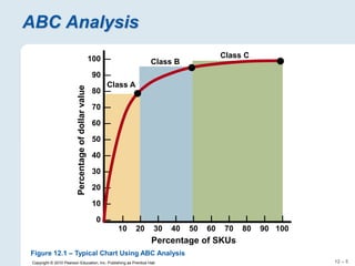
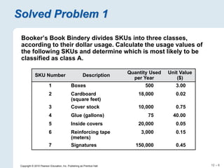
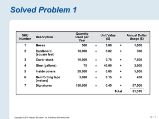
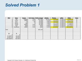
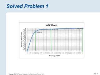
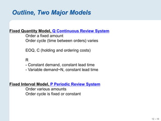
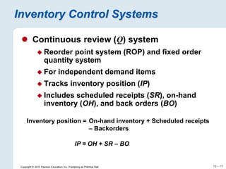
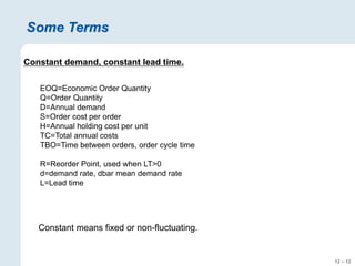
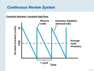
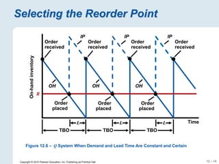
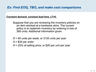
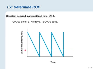
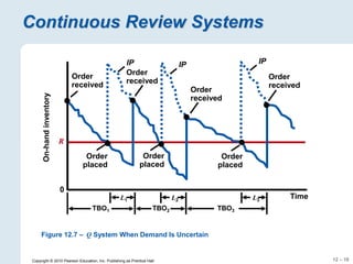
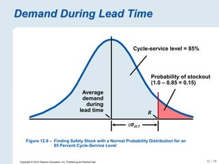
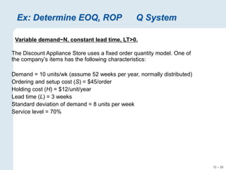
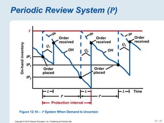
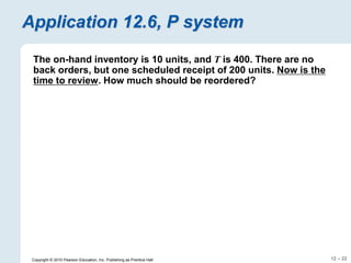
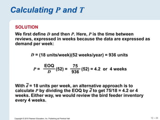
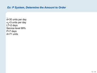
12 – 1
Copyright © 2010 Pearson Education, Inc. Publishing as Prentice Hall.
Inventory Management
12
For Operations Management, 9e by
Krajewski/Ritzman/Malhotra
© 2010 Pearson Education
Homework: 1, 3(assume 250
working days/year), 5, 7, 10, 13,
Milligan Workshop
12 – 2
Inventory Management
 Concepts
 Weeks of supply
 Turns
 ABC Analysis
 Q System
 Q Systems Total Costs
 P System
 Q System vs. P System
12 – 3
Inventory Management
 Inventory is a stock of anything held to meet some
future demand. It is created when the rate of receipts
exceeds the rate of disbursements.
 A stock or store of goods.
 Inventory Turns (Turnover)
COGS/Avg. Inventory Investment
12 – 4
Inventory Management
 Weeks of supply = Average aggregate Inventory Value / Weekly Sales (at cost)
 IT = COGS / Average aggregate inventory value
 The Eagle Machine Company averaged $2M in inventory last year, and the
COGS was $10M. If the company has 52 business weeks per year, how many
weeks of supply are held in inventory? What is the inventory turnover rate?
12 – 5
Copyright © 2010 Pearson Education, Inc. Publishing as Prentice Hall.
10 20 30 40 50 60 70 80 90 100
Percentage of SKUs
Percentage
of
dollar
value
100 —
90 —
80 —
70 —
60 —
50 —
40 —
30 —
20 —
10 —
0 —
Class C
Class A
Class B
ABC Analysis
Figure 12.1 – Typical Chart Using ABC Analysis
12 – 6
Copyright © 2010 Pearson Education, Inc. Publishing as Prentice Hall.
Solved Problem 1
Booker’s Book Bindery divides SKUs into three classes,
according to their dollar usage. Calculate the usage values of
the following SKUs and determine which is most likely to be
classified as class A.
SKU Number Description
Quantity Used
per Year
Unit Value
($)
1 Boxes 500 3.00
2 Cardboard
(square feet)
18,000 0.02
3 Cover stock 10,000 0.75
4 Glue (gallons) 75 40.00
5 Inside covers 20,000 0.05
6 Reinforcing tape
(meters)
3,000 0.15
7 Signatures 150,000 0.45
12 – 7
Copyright © 2010 Pearson Education, Inc. Publishing as Prentice Hall.
Solved Problem 1
SKU
Number
Description
Quantity
Used per
Year
Unit Value
($)
Annual Dollar
Usage ($)
1 Boxes 500  3.00 = 1,500
2 Cardboard
(square feet)
18,000  0.02 = 360
3 Cover stock 10,000  0.75 = 7,500
4 Glue (gallons) 75  40.00 = 3,000
5 Inside covers 20,000  0.05 = 1,000
6 Reinforcing tape
(meters)
3,000  0.15 = 450
7 Signatures 150,000  0.45 = 67,500
Total 81,310
12 – 8
Copyright © 2010 Pearson Education, Inc. Publishing as Prentice Hall.
Solved Problem 1
12 – 9
Copyright © 2010 Pearson Education, Inc. Publishing as Prentice Hall.
Solved Problem 1
12 – 10
Outline, Two Major Models
Fixed Quantity Model, Q Continuous Review System
Order a fixed amount
Order cycle (time between orders) varies
EOQ, C (holding and ordering costs)
R
- Constant demand, constant lead time
- Variable demand~N, constant lead time
Fixed Interval Model, P Periodic Review System
Order various amounts
Order cycle is fixed or constant
12 – 11
Copyright © 2010 Pearson Education, Inc. Publishing as Prentice Hall.
Inventory Control Systems
 Continuous review (Q) system
 Reorder point system (ROP) and fixed order
quantity system
 For independent demand items
 Tracks inventory position (IP)
 Includes scheduled receipts (SR), on-hand
inventory (OH), and back orders (BO)
Inventory position = On-hand inventory + Scheduled receipts
– Backorders
IP = OH + SR – BO
12 – 12
Some Terms
Constant demand, constant lead time.
EOQ=Economic Order Quantity
Q=Order Quantity
D=Annual demand
S=Order cost per order
H=Annual holding cost per unit
TC=Total annual costs
TBO=Time between orders, order cycle time
R=Reorder Point, used when LT>0
d=demand rate, dbar mean demand rate
L=Lead time
Constant means fixed or non-fluctuating.
12 – 13
Continuous Review System
Constant demand, constant lead time.
On-hand
inventory
(units)
Time
Average
cycle
inventory
Q
Q
—
2
1 cycle
Receive
order
Inventory depletion
(demand rate)
12 – 14
Copyright © 2010 Pearson Education, Inc. Publishing as Prentice Hall.
Selecting the Reorder Point
Time
On-hand
inventory
TBO TBO
L L
TBO
L
Order
placed
Order
placed
Order
placed
IP IP
IP
R
OH OH
OH
Order
received
Order
received
Order
received
Order
received
Figure 12.6 – Q System When Demand and Lead Time Are Constant and Certain
12 – 15
Continuous Review Systems – Total Costs
Constant demand, constant lead time.
12 – 16
Ex: Find EOQ, TBO, and make cost comparisons
Constant demand, constant lead time, LT=0.
Suppose that you are reviewing the inventory policies on
an item stocked at a hardware store. The current
policy is to replenish inventory by ordering in lots of
360 units. Additional information given:
D = 60 units per week, or 3120 units per year
S = $30 per order
H = 25% of selling price, or $20 per unit per year
12 – 17
Ex: Determine ROP
Constant demand, constant lead time, LT>0.
Q=300 units, LT=8 days, TBO=30 days.
On-hand
inventory
(units)
Time
R
12 – 18
Copyright © 2010 Pearson Education, Inc. Publishing as Prentice Hall.
Continuous Review Systems
Time
On-hand
inventory
TBO1 TBO2 TBO3
L1 L2 L3
R
Order
received
Order
placed
Order
placed
Order
received
IP IP
Order
placed
Order
received
Order
received
0
IP
Figure 12.7 – Q System When Demand Is Uncertain
12 – 19
Copyright © 2010 Pearson Education, Inc. Publishing as Prentice Hall.
Demand During Lead Time
Average
demand
during
lead time
Cycle-service level = 85%
Probability of stockout
(1.0 – 0.85 = 0.15)
zσdLT
R
Figure 12.9 – Finding Safety Stock with a Normal Probability Distribution for an
85 Percent Cycle-Service Level
12 – 20
Ex: Determine EOQ, ROP Q System
Variable demand~N, constant lead time, LT>0.
The Discount Appliance Store uses a fixed order quantity model. One of
the company’s items has the following characteristics:
Demand = 10 units/wk (assume 52 weeks per year, normally distributed)
Ordering and setup cost (S) = $45/order
Holding cost (H) = $12/unit/year
Lead time (L) = 3 weeks
Standard deviation of demand = 8 units per week
Service level = 70%
12 – 21
Copyright © 2010 Pearson Education, Inc. Publishing as Prentice Hall.
Periodic Review System (P)
P P
T
L L L
Protection interval
Time
On-hand
inventory
IP3
IP1
IP2
Order
placed
Order
placed
Order
placed
Order
received
Order
received
Order
received
IP IP
IP
OH OH
Q1
Q2
Q3
Figure 12.10 – P System When Demand Is Uncertain
12 – 22
Copyright © 2010 Pearson Education, Inc. Publishing as Prentice Hall.
Application 12.6, P system
The on-hand inventory is 10 units, and T is 400. There are no
back orders, but one scheduled receipt of 200 units. Now is the
time to review. How much should be reordered?
12 – 23
Copyright © 2010 Pearson Education, Inc. Publishing as Prentice Hall.
Calculating P and T
EXAMPLE 12.7
Again, let us return to the bird feeder example. Recall that
demand for the bird feeder is normally distributed with a mean
of 18 units per week and a standard deviation in weekly demand
of 5 units. The lead time is 2 weeks, and the business operates
52 weeks per year. The Q system developed in Example 12.4
called for an EOQ of 75 units and a safety stock of 9 units for a
cycle-service level of 90 percent. What is the equivalent P
system? Answers are to be rounded to the nearest integer.
12 – 24
Copyright © 2010 Pearson Education, Inc. Publishing as Prentice Hall.
Calculating P and T
SOLUTION
We first define D and then P. Here, P is the time between
reviews, expressed in weeks because the data are expressed as
demand per week:
D = (18 units/week)(52 weeks/year) = 936 units
P = (52) =
EOQ
D
(52) = 4.2 or 4 weeks
75
936
With d = 18 units per week, an alternative approach is to
calculate P by dividing the EOQ by d to get 75/18 = 4.2 or 4
weeks. Either way, we would review the bird feeder inventory
every 4 weeks.
12 – 25
Copyright © 2010 Pearson Education, Inc. Publishing as Prentice Hall.
Calculating P and T
We now find the standard deviation of demand over the
protection interval (P + L) = 6:
Before calculating T, we also need a z value. For a 90 percent
cycle-service level z = 1.28. The safety stock becomes
Safety stock = zσP + L = 1.28(12.25) = 15.68 or 16 units
We now solve for T:
= (18 units/week)(6 weeks) + 16 units = 124 units
T = Average demand during the protection interval + Safety stock
= d(P + L) + safety stock
units
12.25
6
5 



 L
P
d
L
P 

12 – 26
Ex: P System, Determine the Amount to Order
d=30 units per day
d=3 units per day
LT=2 days
Service level 99%
P=7 days
A=71 units
12 – 27
Q Model vs. P Model
12 – 28
Copyright © 2010 Pearson Education, Inc. Publishing as Prentice Hall.
IM in Action Video

Inventory Mgmt solved problem Pearson.pptx

  • 1.
    12 – 1 Copyright© 2010 Pearson Education, Inc. Publishing as Prentice Hall. Inventory Management 12 For Operations Management, 9e by Krajewski/Ritzman/Malhotra © 2010 Pearson Education Homework: 1, 3(assume 250 working days/year), 5, 7, 10, 13, Milligan Workshop
  • 2.
    12 – 2 InventoryManagement  Concepts  Weeks of supply  Turns  ABC Analysis  Q System  Q Systems Total Costs  P System  Q System vs. P System
  • 3.
    12 – 3 InventoryManagement  Inventory is a stock of anything held to meet some future demand. It is created when the rate of receipts exceeds the rate of disbursements.  A stock or store of goods.  Inventory Turns (Turnover) COGS/Avg. Inventory Investment
  • 4.
    12 – 4 InventoryManagement  Weeks of supply = Average aggregate Inventory Value / Weekly Sales (at cost)  IT = COGS / Average aggregate inventory value  The Eagle Machine Company averaged $2M in inventory last year, and the COGS was $10M. If the company has 52 business weeks per year, how many weeks of supply are held in inventory? What is the inventory turnover rate?
  • 5.
    12 – 5 Copyright© 2010 Pearson Education, Inc. Publishing as Prentice Hall. 10 20 30 40 50 60 70 80 90 100 Percentage of SKUs Percentage of dollar value 100 — 90 — 80 — 70 — 60 — 50 — 40 — 30 — 20 — 10 — 0 — Class C Class A Class B ABC Analysis Figure 12.1 – Typical Chart Using ABC Analysis
  • 6.
    12 – 6 Copyright© 2010 Pearson Education, Inc. Publishing as Prentice Hall. Solved Problem 1 Booker’s Book Bindery divides SKUs into three classes, according to their dollar usage. Calculate the usage values of the following SKUs and determine which is most likely to be classified as class A. SKU Number Description Quantity Used per Year Unit Value ($) 1 Boxes 500 3.00 2 Cardboard (square feet) 18,000 0.02 3 Cover stock 10,000 0.75 4 Glue (gallons) 75 40.00 5 Inside covers 20,000 0.05 6 Reinforcing tape (meters) 3,000 0.15 7 Signatures 150,000 0.45
  • 7.
    12 – 7 Copyright© 2010 Pearson Education, Inc. Publishing as Prentice Hall. Solved Problem 1 SKU Number Description Quantity Used per Year Unit Value ($) Annual Dollar Usage ($) 1 Boxes 500  3.00 = 1,500 2 Cardboard (square feet) 18,000  0.02 = 360 3 Cover stock 10,000  0.75 = 7,500 4 Glue (gallons) 75  40.00 = 3,000 5 Inside covers 20,000  0.05 = 1,000 6 Reinforcing tape (meters) 3,000  0.15 = 450 7 Signatures 150,000  0.45 = 67,500 Total 81,310
  • 8.
    12 – 8 Copyright© 2010 Pearson Education, Inc. Publishing as Prentice Hall. Solved Problem 1
  • 9.
    12 – 9 Copyright© 2010 Pearson Education, Inc. Publishing as Prentice Hall. Solved Problem 1
  • 10.
    12 – 10 Outline,Two Major Models Fixed Quantity Model, Q Continuous Review System Order a fixed amount Order cycle (time between orders) varies EOQ, C (holding and ordering costs) R - Constant demand, constant lead time - Variable demand~N, constant lead time Fixed Interval Model, P Periodic Review System Order various amounts Order cycle is fixed or constant
  • 11.
    12 – 11 Copyright© 2010 Pearson Education, Inc. Publishing as Prentice Hall. Inventory Control Systems  Continuous review (Q) system  Reorder point system (ROP) and fixed order quantity system  For independent demand items  Tracks inventory position (IP)  Includes scheduled receipts (SR), on-hand inventory (OH), and back orders (BO) Inventory position = On-hand inventory + Scheduled receipts – Backorders IP = OH + SR – BO
  • 12.
    12 – 12 SomeTerms Constant demand, constant lead time. EOQ=Economic Order Quantity Q=Order Quantity D=Annual demand S=Order cost per order H=Annual holding cost per unit TC=Total annual costs TBO=Time between orders, order cycle time R=Reorder Point, used when LT>0 d=demand rate, dbar mean demand rate L=Lead time Constant means fixed or non-fluctuating.
  • 13.
    12 – 13 ContinuousReview System Constant demand, constant lead time. On-hand inventory (units) Time Average cycle inventory Q Q — 2 1 cycle Receive order Inventory depletion (demand rate)
  • 14.
    12 – 14 Copyright© 2010 Pearson Education, Inc. Publishing as Prentice Hall. Selecting the Reorder Point Time On-hand inventory TBO TBO L L TBO L Order placed Order placed Order placed IP IP IP R OH OH OH Order received Order received Order received Order received Figure 12.6 – Q System When Demand and Lead Time Are Constant and Certain
  • 15.
    12 – 15 ContinuousReview Systems – Total Costs Constant demand, constant lead time.
  • 16.
    12 – 16 Ex:Find EOQ, TBO, and make cost comparisons Constant demand, constant lead time, LT=0. Suppose that you are reviewing the inventory policies on an item stocked at a hardware store. The current policy is to replenish inventory by ordering in lots of 360 units. Additional information given: D = 60 units per week, or 3120 units per year S = $30 per order H = 25% of selling price, or $20 per unit per year
  • 17.
    12 – 17 Ex:Determine ROP Constant demand, constant lead time, LT>0. Q=300 units, LT=8 days, TBO=30 days. On-hand inventory (units) Time R
  • 18.
    12 – 18 Copyright© 2010 Pearson Education, Inc. Publishing as Prentice Hall. Continuous Review Systems Time On-hand inventory TBO1 TBO2 TBO3 L1 L2 L3 R Order received Order placed Order placed Order received IP IP Order placed Order received Order received 0 IP Figure 12.7 – Q System When Demand Is Uncertain
  • 19.
    12 – 19 Copyright© 2010 Pearson Education, Inc. Publishing as Prentice Hall. Demand During Lead Time Average demand during lead time Cycle-service level = 85% Probability of stockout (1.0 – 0.85 = 0.15) zσdLT R Figure 12.9 – Finding Safety Stock with a Normal Probability Distribution for an 85 Percent Cycle-Service Level
  • 20.
    12 – 20 Ex:Determine EOQ, ROP Q System Variable demand~N, constant lead time, LT>0. The Discount Appliance Store uses a fixed order quantity model. One of the company’s items has the following characteristics: Demand = 10 units/wk (assume 52 weeks per year, normally distributed) Ordering and setup cost (S) = $45/order Holding cost (H) = $12/unit/year Lead time (L) = 3 weeks Standard deviation of demand = 8 units per week Service level = 70%
  • 21.
    12 – 21 Copyright© 2010 Pearson Education, Inc. Publishing as Prentice Hall. Periodic Review System (P) P P T L L L Protection interval Time On-hand inventory IP3 IP1 IP2 Order placed Order placed Order placed Order received Order received Order received IP IP IP OH OH Q1 Q2 Q3 Figure 12.10 – P System When Demand Is Uncertain
  • 22.
    12 – 22 Copyright© 2010 Pearson Education, Inc. Publishing as Prentice Hall. Application 12.6, P system The on-hand inventory is 10 units, and T is 400. There are no back orders, but one scheduled receipt of 200 units. Now is the time to review. How much should be reordered?
  • 23.
    12 – 23 Copyright© 2010 Pearson Education, Inc. Publishing as Prentice Hall. Calculating P and T EXAMPLE 12.7 Again, let us return to the bird feeder example. Recall that demand for the bird feeder is normally distributed with a mean of 18 units per week and a standard deviation in weekly demand of 5 units. The lead time is 2 weeks, and the business operates 52 weeks per year. The Q system developed in Example 12.4 called for an EOQ of 75 units and a safety stock of 9 units for a cycle-service level of 90 percent. What is the equivalent P system? Answers are to be rounded to the nearest integer.
  • 24.
    12 – 24 Copyright© 2010 Pearson Education, Inc. Publishing as Prentice Hall. Calculating P and T SOLUTION We first define D and then P. Here, P is the time between reviews, expressed in weeks because the data are expressed as demand per week: D = (18 units/week)(52 weeks/year) = 936 units P = (52) = EOQ D (52) = 4.2 or 4 weeks 75 936 With d = 18 units per week, an alternative approach is to calculate P by dividing the EOQ by d to get 75/18 = 4.2 or 4 weeks. Either way, we would review the bird feeder inventory every 4 weeks.
  • 25.
    12 – 25 Copyright© 2010 Pearson Education, Inc. Publishing as Prentice Hall. Calculating P and T We now find the standard deviation of demand over the protection interval (P + L) = 6: Before calculating T, we also need a z value. For a 90 percent cycle-service level z = 1.28. The safety stock becomes Safety stock = zσP + L = 1.28(12.25) = 15.68 or 16 units We now solve for T: = (18 units/week)(6 weeks) + 16 units = 124 units T = Average demand during the protection interval + Safety stock = d(P + L) + safety stock units 12.25 6 5      L P d L P  
  • 26.
    12 – 26 Ex:P System, Determine the Amount to Order d=30 units per day d=3 units per day LT=2 days Service level 99% P=7 days A=71 units
  • 27.
    12 – 27 QModel vs. P Model
  • 28.
    12 – 28 Copyright© 2010 Pearson Education, Inc. Publishing as Prentice Hall. IM in Action Video