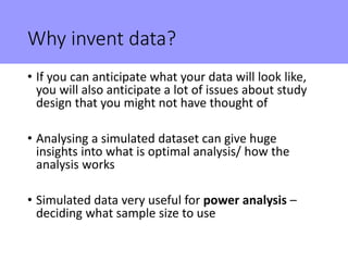
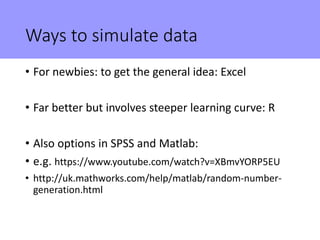
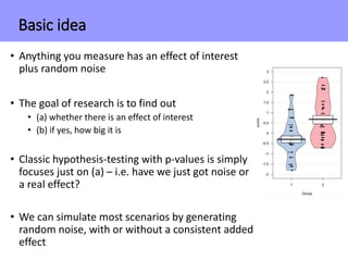
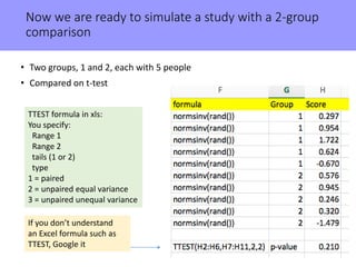
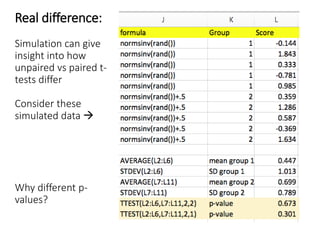
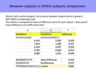
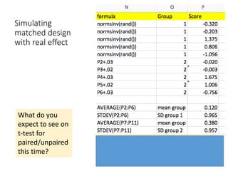
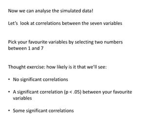
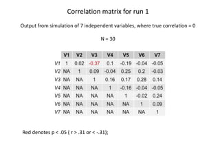
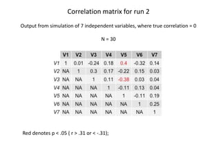
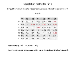
The joys of inventing data:
Using simulations to improve your project
Dorothy V. M. Bishop
Professor of Developmental Neuropsychology
University of Oxford
@deevybee
Why invent data?
• If you can anticipate what your data will look like,
you will also anticipate a lot of issues about study
design that you might not have thought of
• Analysing a simulated dataset can give huge
insights into what is optimal analysis/ how the
analysis works
• Simulated data very useful for power analysis –
deciding what sample size to use
Ways to simulate data
• For newbies: to get the general idea: Excel
• Far better but involves steeper learning curve: R
• Also options in SPSS and Matlab:
• e.g. https://www.youtube.com/watch?v=XBmvYORP5EU
• http://uk.mathworks.com/help/matlab/random-number-
generation.html
Basic idea
• Anything you measure has an effect of interest
plus random noise
• The goal of research is to find out
• (a) whether there is an effect of interest
• (b) if yes, how big it is
• Classic hypothesis-testing with p-values is simply
focuses just on (a) – i.e. have we just got noise or
a real effect?
• We can simulate most scenarios by generating
random noise, with or without a consistent added
effect
Basic idea in Excel
• Generate a bunch of random numbers
• The rand() function generates random numbers between 0
and 1:
N.B. These numbers will change whenever
you open the worksheet, or make any
change to it. To prevent that, select Manual
in Formula|Calculation Options.
For new numbers use Calculate Now button.
Basic idea in Excel
• Generate a bunch of random numbers
• The rand() function generates random numbers between 0
and 1:
N.B. These numbers will change whenever
you open the worksheet, or make any
change to it. To prevent that, select Manual
in Formula|Calculation Options
Are these the kind of numbers
we want?
Normally distributed random numbers
p is area under
curve to left of
given z-score.
z-score: distance from mean in SD units
Normally distributed random numbers
• Nifty way to do this in Excel:
• rand() generates uniform set of values from 0 to 1 – all equally probable
• We can treat these as p-values
• The normsinv() function turns a p-value into a z-score
In practice, do this in just one step with formula: normsinv(rand())
Now we are ready to simulate a study with a 2-group
comparison
• Two groups, 1 and 2, each with 5 people
• Compared on t-test
If you don’t understand
an Excel formula such as
TTEST, Google it
TTEST formula in xls:
You specify:
Range 1
Range 2
tails (1 or 2)
type
1 = paired
2 = unpaired equal variance
3 = unpaired unequal variance
So we’ve generated normally-distributed
values with mean of zero, SD 1 (i.e. z-scores)
for two groups and shown they don’t differ on
t-test
Why is this interesting?!
Introducing a real
group difference
Why isn’t p < .05?
Repeated runs of simulations allow you to see
how statistics vary with the play of chance
• See Geoff Cumming: Dance of the p-values
• https://www.youtube.com/watch?v=5OL1RqHrZQ8
Real difference:
Simulation can give
insight into how
unpaired vs paired t-
tests differ
Consider these
simulated data 
Why different p-
values?
Between-subjects vs Within-subjects comparisons
Paired t-test is within-subjects: the variance between subjects within a group is
NOT USED in computing t-test;
The statistic is computed on basis of difference score for each subject – does overall
mean difference score differ from zero?
• So far, we’ve simulated within-subjects effect using totally random
data.
• What if we simulate data where there is a real effect?
• We can do this by ensuring there is a relationship between data
points for each pair.
Simulating
matched design
with real effect
What do you
expect to see on
t-test for
paired/unpaired
this time?
Simulating
matched design
with real effect
Will results be
different for
paired/unpaired
this time?
Small constant added
to scores of rows 1-5
to generate rows 6-10

Simulating
matched design
with real effect
Do you
understand why
results are so
different this
time?
Why didn’t I always
add .03?
- Consider – what
would be the
variance of the
difference scores?
Getting serious…. moving to R
http://r4ds.had.co.nz/index.html
N.B. This book does not cover simulation: but recommended as good intro to R
http://r4ds.had.co.nz/introduction.html#prerequisites
Gentle introduction to getting up and running for beginners
Using R to simulate correlated variables
Self-teaching scripts on https://osf.io/skz3j/
We’ll start with simulation_ex2_correlations.R
We need to download the package MASS, which has the function mvrnorm
library(MASS) #for mvrnorm function to make multivariate normal
distributed vars
mydata <- mvrnorm(n = myN, rep(myM,nVar), myCov)
Simulates a dataframe of random normal deviates called mydata with:
myN cases
nVar variables
each of which has mean myM (set this to zero for z-scores)
with covariance between variables specified by myCov
Specifying covariance between variables
You should be familiar with the correlation coefficient, r
If we are using z-score and have r = .5, what is covariance?
Specifying covariance for mvrnorm
Let’s say we want variables that are not correlated:
Then myCov would be a little matrix like this:
Off-diagonal values have covariance between variable pairs.
Syntax in R takes getting used to, but we could create this matrix with:
myCov <- matrix(rep(0, nVar*nVar),nrow=nVar) #matrix of nVar zeroes
diag(myCov) <- rep(1,nVar) # now put ones on the diagonal
Putting it all together
myN <- 30
myM <- 0
nVar <- 7
myCov <- matrix(rep(0, nVar*nVar),nrow=nVar) #matrix of nVar zeroes
diag(myCov) <- rep(1, nVar) # now put ones on the diagonal
mydata <- mvrnorm(n = myN, rep(myM,nVar), myCov)
As with Excel simulation, will generate fresh set of numbers on each run, though can
modify the settings to override this.
First six rows of mydata look like this:
Now we can analyse the simulated data!
Let’s look at correlations between the seven variables
Pick your favourite variables by selecting two numbers
between 1 and 7
Thought exercise: how likely is it that we’ll see:
• No significant correlations
• A significant correlation (p < .05) between your favourite
variables
• Some significant correlations
Correlation matrix for run 1
Output from simulation of 7 independent variables, where true correlation = 0
N = 30
Red denotes p < .05 ( r > .31 or < -.31);
Correlation matrix for run 2
Output from simulation of 7 independent variables, where true correlation = 0
N = 30
Red denotes p < .05 ( r > .31 or < -.31);
Correlation matrix for run 3
Output from simulation of 7 independent variables, where true correlation = 0
N = 30
Red denotes p < .05 ( r > .31 or < -.31);
There is no relation between variables – why do we have significant values?
Correlation matrix for run 4
Output from simulation of 7 independent variables, where true correlation = 0
N = 30
Red denotes p < .05 ( r > .31 or < -.31);
We are looking at 21 correlations on each run.
If we use p < .05, then we’re likely to find one significant value per run.
In this case we should be using:
Bonferroni corrected p-value: .05/21 = .002, corresponds to r = .51
Key point: p-values can only be interpreted in terms of the context
in which they are computed
Importance of p < .05 makes sense only in relation to an a-priori
hypothesis
Many ways in which ‘hidden multiplicity’ of testing can give false
positive (p < .05) results
• Data dredging from a large set of variables (as with last
simulation)
• Multi-way Anova with many main effects/interactions
• Trying various analytic approaches until one ‘works’
• Post-hoc division of data into subgroups – ’garden of forking
paths’
Gelman A, and Loken E. 2013.
The garden of forking paths
"El jardín de senderos que se bifurcan"
1 contrast
Probability of a
‘significant’ p-value
< .05 = .05
Large population
database used to explore
link between ADHD and
handedness
https://figshare.com/articles/The_Garden_of_Forking_Paths/2100379
Focus just on Young
subgroup:
2 contrasts at this level
Probability of a
‘significant’ p-value < .05
= .10
Large population
database used to explore
link between ADHD and
handedness
Focus just on Young on
measure of hand skill:
4 contrasts at this level
Probability of a
‘significant’ p-value < .05
= .19
Large population
database used to explore
link between ADHD and
handedness
Focus just on Young,
Females on
measure of hand skill:
8 contrasts at this level
Probability of a
‘significant’ p-value < .05
= .34
Large population
database used to explore
link between ADHD and
handedness
Focus just on Young,
Urban, Females on
measure of hand skill:
16 contrasts at this level
Probability of a
‘significant’ p-value < .05
= .56
Large population
database used to explore
link between ADHD and
handedness
• Simulations help us understand problems of multiple testing,
i.e. how you can get a ‘significant’ result from random data
• Unfortunately a large amount of published literature is
founded on ‘p-hacking’ – testing lots of comparisons and
focusing on the ones that are significant
• This is not OK if there is no correction for multiple testing
• If you find a significant result by data-dredging without any
correction for multiple testing, it needs to be replicated
More discussion and examples on my blog:
http://deevybee.blogspot.co.uk/2012/11/bishopblog-catalogue-updated-24th-nov.html
See sections on Reproducibility and Statistics
• Simulations help us understand problems of multiple testing,
i.e. how you can get a ‘significant’ result from random data
• Simulations are also useful for the opposite situation: showing
how often you can fail to get a significant p-value, even when
there is a true effect
 remember our first simulation in Excel with true effect and non-
significant t-test
• This brings us on to the topic of statistical power
• Power is the probability that, given N and effect size, you will
detect the effect as ‘significant’ in an experiment
• In simple designs can compute power by formula, but can also
use simulations to directly estimate power in any design
Using R to simulate two groups with different means
Self-teaching scripts on https://osf.io/skz3j/
Simulation_ex1_intro.R
# rnorm generates a random sample from a normal distribution
#You have to specify sample size, mean and standard deviation
# Let’s make z-scores for 20 people, so set myN to 20
group1<-rnorm(n = myN, mean = 0, sd = 1)
#Now we’ll do the same for groupB, but their mean is 0.3
group2<-rnorm(n = myN, mean = 0.3, sd = 1)
#We can then run a t-test:
t.test(groupA,groupB)
Results: 10 runs of simulation with N = 20 per group and effect size (d) = .3
** *
*
Can you predict ….
How big a sample would we need to get an 80%
chance of detecting a true effect size of .3?
Results: 10 runs of simulation with N = 100 per group and effect size (d) = .3
**
* * **
* *
Body of table show sample size per group
As shown with simulations, if effect size = .3, then 20 per group is not sufficient for 25% of
runs to give significant result, and 100 per group gives only around 60% significant.
Challenges for experimental design
Minimise false positives
Maximise power – may need collaborative studies for adequate N
Increased N is not only solution. Can also try to maximise effect size:
• Within-subject design (not always better, but worth considering)
• More data per subject to get better estimate of effect
• Better experimental control of dependent variables: use reliable
measures
Post script : Some notes on getting started in R
• General rule #1:if you don't understand something, Google it!
• General rule #2: You learn most when something doesn’t work and you have to
work out why
• General rule #3: you can learn a lot by tweaking a line of script to see what
happens, but always make a copy of the original working script first.
• You need to set your working directory. This determines where output will be
saved and where R will look for data etc. Easiest to do this with
Session|Set Working Directory|To Source File Location
Can also do this with command setwd()
Mac example: setwd (“/Users/dbishop/Dropbox/repcourse”)
PC example: setwd("C:UsersdorothybishopDropboxrepcourse")
• Commands require() and library() load packages you will need. These need to be
installed via Tools|Install Packages. Only need to do that once
Getting started in R
• If program crashes, find source of error by scrolling back in Console to first (red)
error message
• When you select Run in taskbar, it only runs highlighted text (cf. Matlab). This
means you can work through script line by line to see what it does
This won’t, however work for a line that ends in ‘{‘ as script will pause to wait for ‘}’
• Irritating feature of R: it uses '<-' to assign values.
In fact, you can use '=' pretty much anywhere you see '<-’
So ’A <- 3' and ’A= 3' will both assign value of 3 to variable A
R scripts available on : https://osf.io/view/reproducibility2017/
• Simulation_ex1_intro.R
Suitable for R newbies. Demonstrates ‘dance of the p-values’ in a t-test.
Bonus, you learn to make pirate plots
• Simulation_ex2_correlations
Generate correlation matrices from multivariate normal distribution.
Bonus, you learn to use ‘grid’ to make nicely formatted tabular outputs.
• Simulation_ex3_multiwayAnova.R
Simulate data for a 3-way mixed ANOVA. Demonstrates need to correct
for N factors and interactions when doing exploratory multiway Anova.
• Simulation_ex4_multipleReg.R
Simulate data for multiple regression.
• Simulation_ex5_falsediscovery.R
Simulate data for mixture of null and true effects, to demonstrate that
the probability of the data given the hypothesis is different from the
probability of the hypothesis given the data.
Two simulations from Daniel Lakens’ Coursera Course – with notes!
• 1.1 WhichPvaluesCanYouExpect.R
• 3.2 OptionalStoppingSim.R
Now even
more: See
OSF!

Introduction to simulating data to improve your research

  • 1.
    The joys ofinventing data: Using simulations to improve your project Dorothy V. M. Bishop Professor of Developmental Neuropsychology University of Oxford @deevybee
  • 2.
    Why invent data? •If you can anticipate what your data will look like, you will also anticipate a lot of issues about study design that you might not have thought of • Analysing a simulated dataset can give huge insights into what is optimal analysis/ how the analysis works • Simulated data very useful for power analysis – deciding what sample size to use
  • 3.
    Ways to simulatedata • For newbies: to get the general idea: Excel • Far better but involves steeper learning curve: R • Also options in SPSS and Matlab: • e.g. https://www.youtube.com/watch?v=XBmvYORP5EU • http://uk.mathworks.com/help/matlab/random-number- generation.html
  • 4.
    Basic idea • Anythingyou measure has an effect of interest plus random noise • The goal of research is to find out • (a) whether there is an effect of interest • (b) if yes, how big it is • Classic hypothesis-testing with p-values is simply focuses just on (a) – i.e. have we just got noise or a real effect? • We can simulate most scenarios by generating random noise, with or without a consistent added effect
  • 5.
    Basic idea inExcel • Generate a bunch of random numbers • The rand() function generates random numbers between 0 and 1: N.B. These numbers will change whenever you open the worksheet, or make any change to it. To prevent that, select Manual in Formula|Calculation Options. For new numbers use Calculate Now button.
  • 6.
    Basic idea inExcel • Generate a bunch of random numbers • The rand() function generates random numbers between 0 and 1: N.B. These numbers will change whenever you open the worksheet, or make any change to it. To prevent that, select Manual in Formula|Calculation Options Are these the kind of numbers we want?
  • 7.
    Normally distributed randomnumbers p is area under curve to left of given z-score. z-score: distance from mean in SD units
  • 8.
    Normally distributed randomnumbers • Nifty way to do this in Excel: • rand() generates uniform set of values from 0 to 1 – all equally probable • We can treat these as p-values • The normsinv() function turns a p-value into a z-score In practice, do this in just one step with formula: normsinv(rand())
  • 9.
    Now we areready to simulate a study with a 2-group comparison • Two groups, 1 and 2, each with 5 people • Compared on t-test If you don’t understand an Excel formula such as TTEST, Google it TTEST formula in xls: You specify: Range 1 Range 2 tails (1 or 2) type 1 = paired 2 = unpaired equal variance 3 = unpaired unequal variance
  • 10.
    So we’ve generatednormally-distributed values with mean of zero, SD 1 (i.e. z-scores) for two groups and shown they don’t differ on t-test Why is this interesting?!
  • 11.
    Introducing a real groupdifference Why isn’t p < .05?
  • 12.
    Repeated runs ofsimulations allow you to see how statistics vary with the play of chance • See Geoff Cumming: Dance of the p-values • https://www.youtube.com/watch?v=5OL1RqHrZQ8
  • 13.
    Real difference: Simulation cangive insight into how unpaired vs paired t- tests differ Consider these simulated data  Why different p- values?
  • 14.
    Between-subjects vs Within-subjectscomparisons Paired t-test is within-subjects: the variance between subjects within a group is NOT USED in computing t-test; The statistic is computed on basis of difference score for each subject – does overall mean difference score differ from zero?
  • 15.
    • So far,we’ve simulated within-subjects effect using totally random data. • What if we simulate data where there is a real effect? • We can do this by ensuring there is a relationship between data points for each pair.
  • 16.
    Simulating matched design with realeffect What do you expect to see on t-test for paired/unpaired this time?
  • 17.
    Simulating matched design with realeffect Will results be different for paired/unpaired this time? Small constant added to scores of rows 1-5 to generate rows 6-10 
  • 18.
    Simulating matched design with realeffect Do you understand why results are so different this time? Why didn’t I always add .03? - Consider – what would be the variance of the difference scores?
  • 19.
    Getting serious…. movingto R http://r4ds.had.co.nz/index.html N.B. This book does not cover simulation: but recommended as good intro to R
  • 20.
  • 21.
    Using R tosimulate correlated variables Self-teaching scripts on https://osf.io/skz3j/ We’ll start with simulation_ex2_correlations.R We need to download the package MASS, which has the function mvrnorm library(MASS) #for mvrnorm function to make multivariate normal distributed vars mydata <- mvrnorm(n = myN, rep(myM,nVar), myCov) Simulates a dataframe of random normal deviates called mydata with: myN cases nVar variables each of which has mean myM (set this to zero for z-scores) with covariance between variables specified by myCov
  • 22.
    Specifying covariance betweenvariables You should be familiar with the correlation coefficient, r If we are using z-score and have r = .5, what is covariance?
  • 23.
    Specifying covariance formvrnorm Let’s say we want variables that are not correlated: Then myCov would be a little matrix like this: Off-diagonal values have covariance between variable pairs. Syntax in R takes getting used to, but we could create this matrix with: myCov <- matrix(rep(0, nVar*nVar),nrow=nVar) #matrix of nVar zeroes diag(myCov) <- rep(1,nVar) # now put ones on the diagonal
  • 24.
    Putting it alltogether myN <- 30 myM <- 0 nVar <- 7 myCov <- matrix(rep(0, nVar*nVar),nrow=nVar) #matrix of nVar zeroes diag(myCov) <- rep(1, nVar) # now put ones on the diagonal mydata <- mvrnorm(n = myN, rep(myM,nVar), myCov) As with Excel simulation, will generate fresh set of numbers on each run, though can modify the settings to override this. First six rows of mydata look like this:
  • 25.
    Now we cananalyse the simulated data! Let’s look at correlations between the seven variables Pick your favourite variables by selecting two numbers between 1 and 7 Thought exercise: how likely is it that we’ll see: • No significant correlations • A significant correlation (p < .05) between your favourite variables • Some significant correlations
  • 26.
    Correlation matrix forrun 1 Output from simulation of 7 independent variables, where true correlation = 0 N = 30 Red denotes p < .05 ( r > .31 or < -.31);
  • 27.
    Correlation matrix forrun 2 Output from simulation of 7 independent variables, where true correlation = 0 N = 30 Red denotes p < .05 ( r > .31 or < -.31);
  • 28.
    Correlation matrix forrun 3 Output from simulation of 7 independent variables, where true correlation = 0 N = 30 Red denotes p < .05 ( r > .31 or < -.31); There is no relation between variables – why do we have significant values?
  • 29.
    Correlation matrix forrun 4 Output from simulation of 7 independent variables, where true correlation = 0 N = 30 Red denotes p < .05 ( r > .31 or < -.31); We are looking at 21 correlations on each run. If we use p < .05, then we’re likely to find one significant value per run. In this case we should be using: Bonferroni corrected p-value: .05/21 = .002, corresponds to r = .51
  • 30.
    Key point: p-valuescan only be interpreted in terms of the context in which they are computed Importance of p < .05 makes sense only in relation to an a-priori hypothesis Many ways in which ‘hidden multiplicity’ of testing can give false positive (p < .05) results • Data dredging from a large set of variables (as with last simulation) • Multi-way Anova with many main effects/interactions • Trying various analytic approaches until one ‘works’ • Post-hoc division of data into subgroups – ’garden of forking paths’
  • 31.
    Gelman A, andLoken E. 2013. The garden of forking paths "El jardín de senderos que se bifurcan"
  • 32.
    1 contrast Probability ofa ‘significant’ p-value < .05 = .05 Large population database used to explore link between ADHD and handedness https://figshare.com/articles/The_Garden_of_Forking_Paths/2100379
  • 33.
    Focus just onYoung subgroup: 2 contrasts at this level Probability of a ‘significant’ p-value < .05 = .10 Large population database used to explore link between ADHD and handedness
  • 34.
    Focus just onYoung on measure of hand skill: 4 contrasts at this level Probability of a ‘significant’ p-value < .05 = .19 Large population database used to explore link between ADHD and handedness
  • 35.
    Focus just onYoung, Females on measure of hand skill: 8 contrasts at this level Probability of a ‘significant’ p-value < .05 = .34 Large population database used to explore link between ADHD and handedness
  • 36.
    Focus just onYoung, Urban, Females on measure of hand skill: 16 contrasts at this level Probability of a ‘significant’ p-value < .05 = .56 Large population database used to explore link between ADHD and handedness
  • 37.
    • Simulations helpus understand problems of multiple testing, i.e. how you can get a ‘significant’ result from random data • Unfortunately a large amount of published literature is founded on ‘p-hacking’ – testing lots of comparisons and focusing on the ones that are significant • This is not OK if there is no correction for multiple testing • If you find a significant result by data-dredging without any correction for multiple testing, it needs to be replicated More discussion and examples on my blog: http://deevybee.blogspot.co.uk/2012/11/bishopblog-catalogue-updated-24th-nov.html See sections on Reproducibility and Statistics
  • 39.
    • Simulations helpus understand problems of multiple testing, i.e. how you can get a ‘significant’ result from random data • Simulations are also useful for the opposite situation: showing how often you can fail to get a significant p-value, even when there is a true effect  remember our first simulation in Excel with true effect and non- significant t-test • This brings us on to the topic of statistical power • Power is the probability that, given N and effect size, you will detect the effect as ‘significant’ in an experiment • In simple designs can compute power by formula, but can also use simulations to directly estimate power in any design
  • 40.
    Using R tosimulate two groups with different means Self-teaching scripts on https://osf.io/skz3j/ Simulation_ex1_intro.R # rnorm generates a random sample from a normal distribution #You have to specify sample size, mean and standard deviation # Let’s make z-scores for 20 people, so set myN to 20 group1<-rnorm(n = myN, mean = 0, sd = 1) #Now we’ll do the same for groupB, but their mean is 0.3 group2<-rnorm(n = myN, mean = 0.3, sd = 1) #We can then run a t-test: t.test(groupA,groupB)
  • 41.
    Results: 10 runsof simulation with N = 20 per group and effect size (d) = .3 ** * *
  • 42.
    Can you predict…. How big a sample would we need to get an 80% chance of detecting a true effect size of .3?
  • 43.
    Results: 10 runsof simulation with N = 100 per group and effect size (d) = .3 ** * * ** * *
  • 44.
    Body of tableshow sample size per group As shown with simulations, if effect size = .3, then 20 per group is not sufficient for 25% of runs to give significant result, and 100 per group gives only around 60% significant.
  • 45.
    Challenges for experimentaldesign Minimise false positives Maximise power – may need collaborative studies for adequate N Increased N is not only solution. Can also try to maximise effect size: • Within-subject design (not always better, but worth considering) • More data per subject to get better estimate of effect • Better experimental control of dependent variables: use reliable measures
  • 46.
    Post script :Some notes on getting started in R • General rule #1:if you don't understand something, Google it! • General rule #2: You learn most when something doesn’t work and you have to work out why • General rule #3: you can learn a lot by tweaking a line of script to see what happens, but always make a copy of the original working script first. • You need to set your working directory. This determines where output will be saved and where R will look for data etc. Easiest to do this with Session|Set Working Directory|To Source File Location Can also do this with command setwd() Mac example: setwd (“/Users/dbishop/Dropbox/repcourse”) PC example: setwd("C:UsersdorothybishopDropboxrepcourse") • Commands require() and library() load packages you will need. These need to be installed via Tools|Install Packages. Only need to do that once
  • 47.
    Getting started inR • If program crashes, find source of error by scrolling back in Console to first (red) error message • When you select Run in taskbar, it only runs highlighted text (cf. Matlab). This means you can work through script line by line to see what it does This won’t, however work for a line that ends in ‘{‘ as script will pause to wait for ‘}’ • Irritating feature of R: it uses '<-' to assign values. In fact, you can use '=' pretty much anywhere you see '<-’ So ’A <- 3' and ’A= 3' will both assign value of 3 to variable A
  • 48.
    R scripts availableon : https://osf.io/view/reproducibility2017/ • Simulation_ex1_intro.R Suitable for R newbies. Demonstrates ‘dance of the p-values’ in a t-test. Bonus, you learn to make pirate plots • Simulation_ex2_correlations Generate correlation matrices from multivariate normal distribution. Bonus, you learn to use ‘grid’ to make nicely formatted tabular outputs. • Simulation_ex3_multiwayAnova.R Simulate data for a 3-way mixed ANOVA. Demonstrates need to correct for N factors and interactions when doing exploratory multiway Anova. • Simulation_ex4_multipleReg.R Simulate data for multiple regression. • Simulation_ex5_falsediscovery.R Simulate data for mixture of null and true effects, to demonstrate that the probability of the data given the hypothesis is different from the probability of the hypothesis given the data. Two simulations from Daniel Lakens’ Coursera Course – with notes! • 1.1 WhichPvaluesCanYouExpect.R • 3.2 OptionalStoppingSim.R Now even more: See OSF!