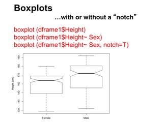
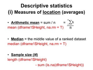
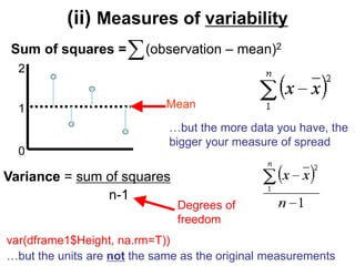
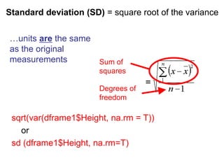
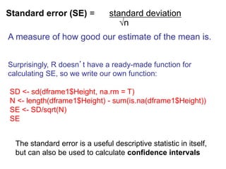
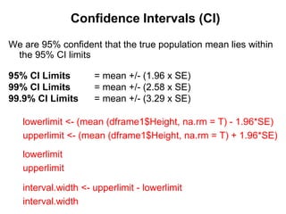
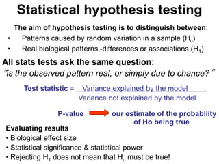
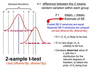
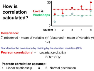
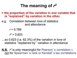
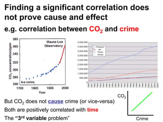
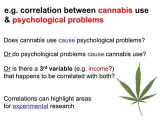
Data analysis with R
statistical software
Dr. Rob Thomas
ļ‚š ThomasRJ@Cardiff.ac.uk
Session 1
Welcome to
the course
Getting started with R
Save the Excel file called ā€œHeights.xlsā€ as a .csv file
Excel > File > Save as > Save as type >
Choose ā€œCSV (Comma delimited)
Save this file as ā€œHeights.csvā€
click on ā€œOKā€ & ā€œyesā€ when prompted
Open the R software on your computer
Ask R to read the heights.csv file
dframe1 <- read.csv(file.choose()) # navigate to your .csv file
names (dframe1) # names of the variables
summary (dframe1) # numerical summary
Histograms
with (dframe1, hist(Height))
hist (dframe1$Height)
Scatterplots
with (dframe1, plot(Age, Height))
plot (dframe1$Height~ dframe1$Age)
abline (lm (dframe1$Height~ dframe1$Age))
?plot # for help files about the ā€œplotā€ function
Plotting graphs
–two ways of specifying variables
Pairwise plots
names(dframe1)
pairs (dframe1[c(1,2,4)],
panel = panel.smooth)
Specifies variables
1, 2 and 4 in
dframe1
Sex
130 150 170 190
1.0
1.2
1.4
1.6
1.8
2.0
130
150
170
190
Height
1.0 1.2 1.4 1.6 1.8 2.0 20 25 30 35
20
25
30
35
Age
Boxplots
…with or without a ā€œnotchā€
boxplot (dframe1$Height)
boxplot (dframe1$Height~ Sex)
boxplot (dframe1$Height~ Sex, notch=T)
Female Male
130
140
150
160
170
180
190
Height
(cm)
Descriptive statistics
(i) Measures of location (averages)
• Arithmetic mean = sum / n =
mean (dframe1$Height, na.rm = T)
• Median = the middle value of a ranked dataset
median (dframe1$Height, na.rm = T)
• Sample size (N)
length (dframe1$Height)
- sum (is.na(dframe1$Height))

1
n
x
n
(ii) Measures of variability
Sum of squares = (observation – mean)2

0
1
2
…but the more data you have, the
bigger your measure of spread
Degrees of
freedom
Variance = sum of squares
n-1
var(dframe1$Height, na.rm=T))
…but the units are not the same as the original measurements
Mean
Standard deviation (SD) = square root of the variance
Sum of
squares
Degrees of
freedom
…units are the same
as the original
measurements
sqrt(var(dframe1$Height, na.rm = T))
or
sd (dframe1$Height, na.rm=T)
Standard error (SE) = standard deviation
ļƒ–n
A measure of how good our estimate of the mean is.
Surprisingly, R doesn’t have a ready-made function for
calculating SE, so we write our own function:
SD <- sd(dframe1$Height, na.rm = T)
N <- length(dframe1$Height) - sum(is.na(dframe1$Height))
SE <- SD/sqrt(N)
SE
The standard error is a useful descriptive statistic in itself,
but can also be used to calculate confidence intervals
Confidence Intervals (CI)
We are 95% confident that the true population mean lies within
the 95% CI limits
95% CI Limits = mean +/- (1.96 x SE)
99% CI Limits = mean +/- (2.58 x SE)
99.9% CI Limits = mean +/- (3.29 x SE)
lowerlimit <- (mean (dframe1$Height, na.rm = T) - 1.96*SE)
upperlimit <- (mean (dframe1$Height, na.rm = T) + 1.96*SE)
lowerlimit
upperlimit
interval.width <- upperlimit - lowerlimit
interval.width
Statistical hypothesis testing
All stats tests ask the same question:
ā€œis the observed pattern real, or simply due to chance?ā€
Test statistic = Variance explained by the model .
Variance not explained by the model
P-value our estimate of the probability
of Ho being true
The aim of hypothesis testing is to distinguish between:
• Patterns caused by random variation in a sample (Ho)
• Real biological patterns -differences or associations (H1)
Evaluating results
• Biological effect size
• Statistical significance & statistical power
• Rejecting H1 does not mean that Ho must be true!
-1 1
-2 2
-3 3
Standard Deviations t = difference between the 2 means
random variation within each group
t = mean1 – mean2
Estimate of SE
2-sample t-test
t.test (dframe1$x, dframe1$y)
Assumptions of
t-tests
1.Normal
distributions
2.Equal variances
-1 1
-2 2
-3 3
Standard Deviations t = difference between the 2 means
random variation within each group
t = mean1 – mean2
Estimate of SE
• If t = 0, Ho is likely to be true
• If t is very large, Ho is
unlikely to be true.
• Compare observed value of
t, with the t-
distribution for the
relevant degrees of
freedom, to obtain the
prob. of Ho being true.
Pooled SE if variances are equal
Separate SE if variances are unequal
var.test (dframe1$x, dframe1$y)
2-sample t-test
t.test (dframe1$x, dframe1$y)
How does a
t-test work?
Exercise:
The Dr Ian Vaughan
Memorial Spreadsheet
The master at work:
Ian collecting data for his next t-test
Excel file in:
Session 1 folder
Left hand side:
Checking for normal distributions
Checking for homogeneity of variances
Right hand side:
t-test for equal variances
t-test for unequal variances
Reporting a t-test
There are 5 things that you must ALWAYS state when reporting a
statistical test:
1. Name of the test E.g. 2-sample t-test
1-tailed or 2-tailed test? 2-tailed test
2. Value of the test statistic t = 5.164
3. Sample sizes n = 119, 186
or degrees of freedom d.f. = 303
4. Statistical significance P < 0.0001
i.e. a significant difference between male and female heights
5. Effect size and direction (means ± Confidence Intervals)
Males = 168.2cm (166.5-169.8), Females = 159.8cm (158.1-161.3)
Things to consider when evaluating
the test of a hypothesis
1. Effect size
Is the size of the effect important?
2. Statistical significance
P = probability the Ho is true
Accept or reject Ho
P = 0.05 is the conventional cut-off between significant
and non-significant effects, but this is arbitrary!
e.g. P = 0.0499 is marginally significant
but P = 0.0501 is marginally non-significant
…even though these 2 results are nearly identical
3. Statistical power
Lectures attended
10
8
6
4
2
0
100
80
60
40
20
0
No. of stats workshops attended
18
16
14
12
10
8
6
4
2
0
30
25
20
15
10
5
0
Workshops attended
Love
of
statistics
Question: Is this just
random variation?
(Ho)
Or are these statistically
significant patterns?
(HA)
Association = a relationship or correlation
i.e. What is the probability of finding these patterns if there is
no real relationship between the 2 variables?
Tests for associations between 2
continuous variables
How is
correlation
calculated?
Pearson correlation assumes:
1. Linear relationship & 2. Normal distribution
Covariance:
 (observed - mean of variable x)* (observed – mean of variable y)
n -1
Standardise the covariance by dividing by the standard deviation (SD)
Pearson correlation r = covariance of x & y
SDx * SDy
Student 1 2 3 4 5
Love &
Workshops
0
30
plot (x,y)
Positive relationship
Negative relationship
No correlation
Weak negative
relationship
Non-linear relationship?
–Try transforming one or both variables to make the relationship linear
Assumption 1: Linear relationship?
r = +1
r = -1
r = 0
r = -0.4
r = correlation
coefficient
Assumption 2: Normal distributions?
If the data are normally distributed, or can be transformed
(squashed) to be normally distributed, use a
Pearson’s correlation
Otherwise, use a Spearman’s rank correlation
…or a Kendall’s tau correlation with small sample sizes (n<7)
and/or lots of tied ranks
How to test for correlations
To do a Pearson correlation:
cor.test (dframe1$x, dframe1$y)
To do a Spearman rank or Kendall’s tau correlation:
cor.test (dframe1$x, dframe1$y, method = ā€œspearmanā€)
cor.test (dframe1$x, dframe1$y, method = ā€œkendallā€)
Reporting correlations
There are 6 things that you must ALWAYS state when reporting a
statistical test:
1. Name of the test E.g. Pearson’s correlation
2. 1-tailed or 2-tailed test? 2-tailed test
3. Value of the test statistic r = 0.789
4. Sample size n = 18
or degrees of freedom d.f. = 16
5. Statistical significance P < 0.0001
i.e. a highly significant positive correlation
6. Effect size (note that the correlation coefficient r is also a
measure of the effect size / strength of the relationship)
The meaning of r2
= the proportion of the variation in one variable that
is ā€œexplainedā€ by variation in the other.
e.g. Correlation between love of statistics
and attendance
r = 0.789
r2 = 0.623
…so 0.623 (i.e. 62.3%) of the variation in love of
statistics ā€œexplained byā€ variation in attendance
N.B. r2 is only meaningful for Pearson’s correlation r,
not for Spearman’s rank or Kendall’s tau correlations
Finding a significant correlation does
not prove cause and effect
e.g. correlation between CO2 and crime
But CO2 does not cause crime (or vice-versa)
Both are positively correlated with time
The ā€œ3rd variable problemā€
CO2
Crime
e.g. correlation between cannabis use
& psychological problems
Does cannabis use cause psychological problems?
Or do psychological problems cause cannabis use?
Or is there a 3rd variable (e.g. income?)
that happens to be correlated with both?
Correlations can highlight areas
for experimental research

Session 1 -Getting started with R Statistics package.ppt

  • 1.
    Data analysis withR statistical software Dr. Rob Thomas ļ‚š ThomasRJ@Cardiff.ac.uk Session 1 Welcome to the course
  • 2.
    Getting started withR Save the Excel file called ā€œHeights.xlsā€ as a .csv file Excel > File > Save as > Save as type > Choose ā€œCSV (Comma delimited) Save this file as ā€œHeights.csvā€ click on ā€œOKā€ & ā€œyesā€ when prompted Open the R software on your computer Ask R to read the heights.csv file dframe1 <- read.csv(file.choose()) # navigate to your .csv file names (dframe1) # names of the variables summary (dframe1) # numerical summary
  • 3.
    Histograms with (dframe1, hist(Height)) hist(dframe1$Height) Scatterplots with (dframe1, plot(Age, Height)) plot (dframe1$Height~ dframe1$Age) abline (lm (dframe1$Height~ dframe1$Age)) ?plot # for help files about the ā€œplotā€ function Plotting graphs –two ways of specifying variables
  • 4.
    Pairwise plots names(dframe1) pairs (dframe1[c(1,2,4)], panel= panel.smooth) Specifies variables 1, 2 and 4 in dframe1 Sex 130 150 170 190 1.0 1.2 1.4 1.6 1.8 2.0 130 150 170 190 Height 1.0 1.2 1.4 1.6 1.8 2.0 20 25 30 35 20 25 30 35 Age
  • 5.
    Boxplots …with or withouta ā€œnotchā€ boxplot (dframe1$Height) boxplot (dframe1$Height~ Sex) boxplot (dframe1$Height~ Sex, notch=T) Female Male 130 140 150 160 170 180 190 Height (cm)
  • 6.
    Descriptive statistics (i) Measuresof location (averages) • Arithmetic mean = sum / n = mean (dframe1$Height, na.rm = T) • Median = the middle value of a ranked dataset median (dframe1$Height, na.rm = T) • Sample size (N) length (dframe1$Height) - sum (is.na(dframe1$Height))  1 n x n
  • 7.
    (ii) Measures ofvariability Sum of squares = (observation – mean)2  0 1 2 …but the more data you have, the bigger your measure of spread Degrees of freedom Variance = sum of squares n-1 var(dframe1$Height, na.rm=T)) …but the units are not the same as the original measurements Mean
  • 8.
    Standard deviation (SD)= square root of the variance Sum of squares Degrees of freedom …units are the same as the original measurements sqrt(var(dframe1$Height, na.rm = T)) or sd (dframe1$Height, na.rm=T)
  • 9.
    Standard error (SE)= standard deviation ļƒ–n A measure of how good our estimate of the mean is. Surprisingly, R doesn’t have a ready-made function for calculating SE, so we write our own function: SD <- sd(dframe1$Height, na.rm = T) N <- length(dframe1$Height) - sum(is.na(dframe1$Height)) SE <- SD/sqrt(N) SE The standard error is a useful descriptive statistic in itself, but can also be used to calculate confidence intervals
  • 10.
    Confidence Intervals (CI) Weare 95% confident that the true population mean lies within the 95% CI limits 95% CI Limits = mean +/- (1.96 x SE) 99% CI Limits = mean +/- (2.58 x SE) 99.9% CI Limits = mean +/- (3.29 x SE) lowerlimit <- (mean (dframe1$Height, na.rm = T) - 1.96*SE) upperlimit <- (mean (dframe1$Height, na.rm = T) + 1.96*SE) lowerlimit upperlimit interval.width <- upperlimit - lowerlimit interval.width
  • 11.
    Statistical hypothesis testing Allstats tests ask the same question: ā€œis the observed pattern real, or simply due to chance?ā€ Test statistic = Variance explained by the model . Variance not explained by the model P-value our estimate of the probability of Ho being true The aim of hypothesis testing is to distinguish between: • Patterns caused by random variation in a sample (Ho) • Real biological patterns -differences or associations (H1) Evaluating results • Biological effect size • Statistical significance & statistical power • Rejecting H1 does not mean that Ho must be true!
  • 12.
    -1 1 -2 2 -33 Standard Deviations t = difference between the 2 means random variation within each group t = mean1 – mean2 Estimate of SE 2-sample t-test t.test (dframe1$x, dframe1$y) Assumptions of t-tests 1.Normal distributions 2.Equal variances
  • 13.
    -1 1 -2 2 -33 Standard Deviations t = difference between the 2 means random variation within each group t = mean1 – mean2 Estimate of SE • If t = 0, Ho is likely to be true • If t is very large, Ho is unlikely to be true. • Compare observed value of t, with the t- distribution for the relevant degrees of freedom, to obtain the prob. of Ho being true. Pooled SE if variances are equal Separate SE if variances are unequal var.test (dframe1$x, dframe1$y) 2-sample t-test t.test (dframe1$x, dframe1$y)
  • 14.
    How does a t-testwork? Exercise: The Dr Ian Vaughan Memorial Spreadsheet The master at work: Ian collecting data for his next t-test Excel file in: Session 1 folder Left hand side: Checking for normal distributions Checking for homogeneity of variances Right hand side: t-test for equal variances t-test for unequal variances
  • 15.
    Reporting a t-test Thereare 5 things that you must ALWAYS state when reporting a statistical test: 1. Name of the test E.g. 2-sample t-test 1-tailed or 2-tailed test? 2-tailed test 2. Value of the test statistic t = 5.164 3. Sample sizes n = 119, 186 or degrees of freedom d.f. = 303 4. Statistical significance P < 0.0001 i.e. a significant difference between male and female heights 5. Effect size and direction (means ± Confidence Intervals) Males = 168.2cm (166.5-169.8), Females = 159.8cm (158.1-161.3)
  • 16.
    Things to considerwhen evaluating the test of a hypothesis 1. Effect size Is the size of the effect important? 2. Statistical significance P = probability the Ho is true Accept or reject Ho P = 0.05 is the conventional cut-off between significant and non-significant effects, but this is arbitrary! e.g. P = 0.0499 is marginally significant but P = 0.0501 is marginally non-significant …even though these 2 results are nearly identical 3. Statistical power
  • 17.
    Lectures attended 10 8 6 4 2 0 100 80 60 40 20 0 No. ofstats workshops attended 18 16 14 12 10 8 6 4 2 0 30 25 20 15 10 5 0 Workshops attended Love of statistics Question: Is this just random variation? (Ho) Or are these statistically significant patterns? (HA) Association = a relationship or correlation i.e. What is the probability of finding these patterns if there is no real relationship between the 2 variables? Tests for associations between 2 continuous variables
  • 18.
    How is correlation calculated? Pearson correlationassumes: 1. Linear relationship & 2. Normal distribution Covariance:  (observed - mean of variable x)* (observed – mean of variable y) n -1 Standardise the covariance by dividing by the standard deviation (SD) Pearson correlation r = covariance of x & y SDx * SDy Student 1 2 3 4 5 Love & Workshops 0 30
  • 19.
    plot (x,y) Positive relationship Negativerelationship No correlation Weak negative relationship Non-linear relationship? –Try transforming one or both variables to make the relationship linear Assumption 1: Linear relationship? r = +1 r = -1 r = 0 r = -0.4 r = correlation coefficient
  • 20.
    Assumption 2: Normaldistributions? If the data are normally distributed, or can be transformed (squashed) to be normally distributed, use a Pearson’s correlation Otherwise, use a Spearman’s rank correlation …or a Kendall’s tau correlation with small sample sizes (n<7) and/or lots of tied ranks How to test for correlations To do a Pearson correlation: cor.test (dframe1$x, dframe1$y) To do a Spearman rank or Kendall’s tau correlation: cor.test (dframe1$x, dframe1$y, method = ā€œspearmanā€) cor.test (dframe1$x, dframe1$y, method = ā€œkendallā€)
  • 21.
    Reporting correlations There are6 things that you must ALWAYS state when reporting a statistical test: 1. Name of the test E.g. Pearson’s correlation 2. 1-tailed or 2-tailed test? 2-tailed test 3. Value of the test statistic r = 0.789 4. Sample size n = 18 or degrees of freedom d.f. = 16 5. Statistical significance P < 0.0001 i.e. a highly significant positive correlation 6. Effect size (note that the correlation coefficient r is also a measure of the effect size / strength of the relationship)
  • 22.
    The meaning ofr2 = the proportion of the variation in one variable that is ā€œexplainedā€ by variation in the other. e.g. Correlation between love of statistics and attendance r = 0.789 r2 = 0.623 …so 0.623 (i.e. 62.3%) of the variation in love of statistics ā€œexplained byā€ variation in attendance N.B. r2 is only meaningful for Pearson’s correlation r, not for Spearman’s rank or Kendall’s tau correlations
  • 23.
    Finding a significantcorrelation does not prove cause and effect e.g. correlation between CO2 and crime But CO2 does not cause crime (or vice-versa) Both are positively correlated with time The ā€œ3rd variable problemā€ CO2 Crime
  • 24.
    e.g. correlation betweencannabis use & psychological problems Does cannabis use cause psychological problems? Or do psychological problems cause cannabis use? Or is there a 3rd variable (e.g. income?) that happens to be correlated with both? Correlations can highlight areas for experimental research