Applied machine learning Diet_IML_Unit-3.pdf

Syllabus of IML
• Unit III: Statistical Learning: Machine Learning and Inferential Statistical Analysis,
Descriptive Statistics in learning techniques, Bayesian Reasoning: A probabilistic
approach to inference, K-Nearest Neighbor Classifier. Discriminant functions and
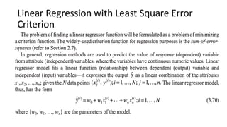
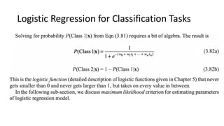
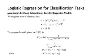
regression functions, Linear Regression with Least Square Error Criterion, Logistic
Regression for Classification Tasks, Fisher's Linear Discriminant and Thresholding
for Classification, Minimum Description Length Principle.
• Text Books:
1. Applied Machine Learning,1st edition, M.Gopal, McGraw Hill Education,2018

Machine Learning and Inferential Statistical
Analysis
▪ Statistical analysis saw the development of two branches in the 18th century—
Bayesian and classical statistics.
▪ Statistical analysis approach that originated from the mathematical works of
Thomas Bayes, analysis is based on the concept of conditional probability: the
probability of an event taking place considering that another event has already
taken place.
▪ Regression and correlation were concepts that were developed in the later part
of the 19th century, for generic data analysis.
▪ A system developed for inference testing in medical sciences, by RA Fisher in
the 1920s was based on the concept of standard deviation.

Analysis
▪ Mathematical research dominated the 1980s similar to Fisher’s statistical
inference through the development of nonlinear versions of parametric
techniques.
▪ Machine learning methods allowed the analysis of extremely nonlinear
relationships in big datasets which have no known distribution.
▪ Conventional statistical analysis adopts the deductive technique to look for
relationships in datasets. It employs past knowledge (domain theory) along with
training examples to create a model.
▪ Machine learning methods, on the other hand, adopt the inductive technique to
discover feeble patterns of relationships in datasets.

Analysis
▪ Inferential statistics is concerned with making predictions from data.
▪ In this chapter, we introduce Bayesian learning, giving detailed coverage of naive Bayes
classifier, and k-Nearest Neighbor (k-NN) classifier.
▪ The inference techniques based on classical parametric statistics: linear regression,
logistic regression, discriminant analysis; are also covered in this chapter.
▪ The other topic based on statistical techniques included in this chapter is Minimum
Description Length (MDL) principle.

Descriptive Statistics in learning techniques
▪ The standard ‘hard-computing’ paradigm is based on analytical closed-form
models using a reasonable number of equations that can solve the given
problem in a reasonable time, at reasonable cost, and with reasonable
accuracy. It is a mathematically well-established discipline.
▪ The field of machine learning is also mathematically well-founded; it uses ‘soft-
models’— modern computer-based applications of standard and novel
mathematical and statistical techniques. Each of these techniques collects
inputs from linear algebra and analytical geometry, vector calculus,
unconstrained optimization, constrained optimization, probability theory and
information theory.

Representing Uncertainties in Data: Probability
Distributions
▪ Common features of existing information for machine learning is the
uncertainty associated with it.
▪ Real-world data tend to remain incomplete, noisy, and inconsistent.
Noise, missing values, and inconsistencies add to the inaccuracy of data.
▪ Information, in other words, is not always suitable for solving problems.
However, machine intelligence can tackle these defects and can usually make
the right judgments and decisions.
▪ Intelligent systems should possess the capability to deal with uncertainties and
derive conclusions.
▪ Most popular uncertainty management paradigms are based on probability
theory. Probability can be viewed as a numerical measure of the likelihood of
occurrence of an outcome relative to the set of other alternatives.

Probability Mass Function (discrete random
variable)
▪ Assume n = 1, and the feature x is a random variable representing a sample point.
Random variable x can be discrete or continuous. When x is discrete, it can
possess finite number of discrete values vlx; l = 1, 2,…, d. The occurrence of
discrete value vlx of the random variable x is expressed by the probability P(x = vlx).
▪

probability density function
▪ A continuous random variable can take infinite values within its domain.
▪ In this case, the probability of a particular value within the domain is zero.
▪ Thus, we describe a continuous random variable not by the probability of taking on a
certain value but by probability of being within a range of values.
▪ For a continuous random variable x, probabilities are associated with the ranges of
values of the variable, and consequently, at the specific value of x, only the density
of probability is defined.
▪ If p(x) is the probability density function1 of x, the probability of x being in the interval
(v1x, v2x) is:

Class-conditional probability density function

Descriptive measures of probability
distributions

Descriptive Measures from Data Sample
▪ A statistic is a measure of a sample of data. Statistics is the study of these
measures and the samples they are measured on. Let us summarize the
simplest statistical measures employed in data exploration.
▪ Range: It is the difference between the smallest and the largest observation in
the sample. It is frequently examined along with the minimum and
maximum values themselves.
▪ Mean: It is the arithmetic average value, that is, the sum of all the values
divided by the number of values.
▪ Median: The median value divides the observations into two groups of equal
size—one possessing values smaller than the median and another one
possessing values bigger than the median

▪ Mode: The value that occurs most often, is called the mode of data sample.
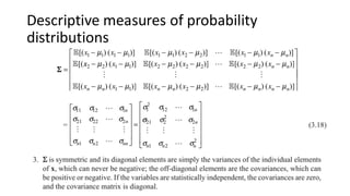
▪ Variance and Standard Deviation: The difference between a given observation
and the arithmetic average of the sample is called its deviation. The
variance is defined as the arithmetic average of the squares of the
deviations. It is a measure of dispersion of data values; measures how
closely the values cluster around their arithmetic average value. A
low variance means that the values stay near the arithmetic average; a
high variance means the opposite.
▪ Standard deviation is the square root of the variance and is commonly employed
in measuring dispersion. It is expressed in units similar to the values
themselves while variance is expressed in terms of those units squared.

Data Similarity
▪ Characterizing the similarity of the patterns in state space can be done through
some form of metric (distance) measure: distance between two vectors is a
measure of similarity between two corresponding patterns. Many measures of
‘distance’ have been proposed in the literature.

Bayesian Reasoning: A probabilistic approach
to inference

Discriminant functions and regression
functions
▪ To represent pattern classifiers is in terms of discriminant functions.
▪ The patterns are feature vectors x(i); i = 1, …, N, and class labels yq; q = 1, 2,
…, M.
▪ The Bayesian approach to classification assumes that the problem of
pattern classification can be expressed in probabilistic terms and that a
priori probabilities P(yq) and the conditional probability-density functions
p(x|yq); q = 1, … M, are known.
▪ The posterior probability P(yq|x) is sought for classifying objects into
corresponding classes. This probability can be expressed in the form of
Bayes rule

functions
▪ A pattern classifier assigns the feature vector x to one of the number of possible
classes yq; and in this way partitions feature space into line segments, areas,
volumes, and hyper volumes, which are decision regions in the case of one-, two-
, three-, or higher-dimensional feature space, respectively.

functions

Practical Hypothesis functions
Heuristic search is organized as per the following two-step procedure.
(i) The search is first focused on a hypothesis class chosen for the learning task in hand.
The different hypotheses classes are appropriate for learning different kinds of functions.
The main hypotheses classes are:
1. Linear Models
2. Logistic Models
3. Support Vector Machines
4. Neural Networks
5. Fuzzy Logic Models
6. Decisions Trees
7. k-Nearest Neighbors (k-NN)
8. Naive Bayes

Practical Hypothesis functions

Linear Regression with Least Square Error
Criterion

Least Mean Square (LMS) Algorithm

Logistic Regression for Classification Tasks

Fisher's Linear Discriminant and Thresholding
for Classification

Thresholding for Classification

Applied machine learning Diet_IML_Unit-3.pdf

More Related Content

Similar to Applied machine learning Diet_IML_Unit-3.pdf

More from bandiprathyu

Recently uploaded

Applied machine learning Diet_IML_Unit-3.pdf