Downloaded 160 times
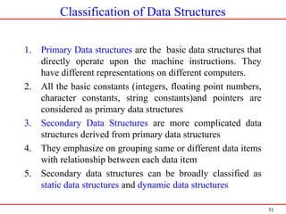
![47
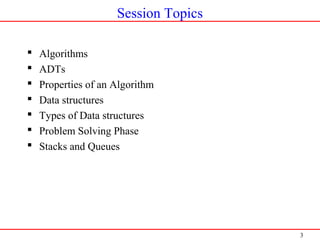
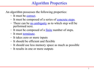
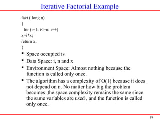
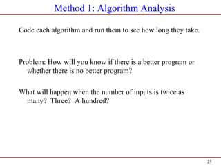
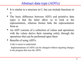
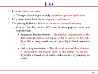
Insert/ Push Operation
Inserting an element into the stack is called push operation.
Function to insert an item: (Push )
void push(int item, int *top, int s[])
{
if(*top == STACKSIZE - 1) /*Is stack empty?*/
{
printf(“Stack Overflown”);
return;
}
/* Increment top and then insert an item*/
s[++(*top)] = item;
}](https://image.slidesharecdn.com/introductiontodatastructures-140603122653-phpapp02/85/Introduction-to-data-structures-and-Algorithm-47-320.jpg)
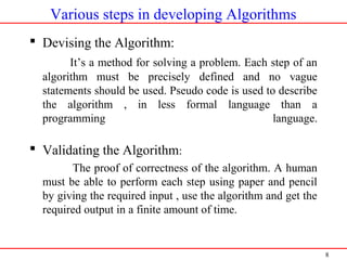
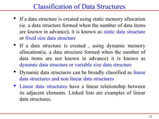
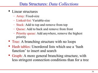
![48
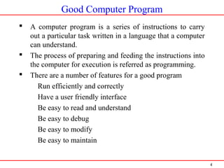
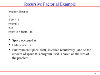
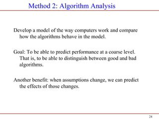
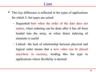
Delete/Pop Operation
Deleting an element from the stack is called pop operation.
Function to delete an item: (Pop )
int pop(int *top, int s[])
{
int item_deleted /*Holds the top most item */
if(*top == -1)
{
return 0; /*Indicates empty stack*/
}
/*Obtain the top most element and change the position
of top item */
item_deleted=s[(*top)--];
/*Send to the calling function*/
return item_deleted;
}](https://image.slidesharecdn.com/introductiontodatastructures-140603122653-phpapp02/85/Introduction-to-data-structures-and-Algorithm-48-320.jpg)
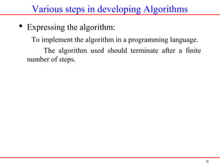
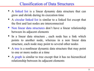
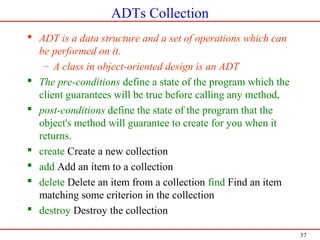
![49
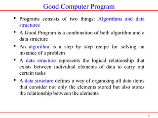
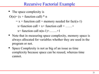
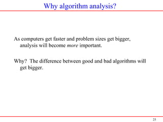
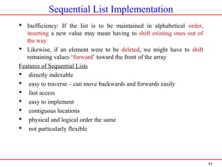
Display Procedure
If the stack already has some elements, all those items are displayed one
after the other.
void display(int top, int s[]){
int i;
if(top == -1) /* Is stack empty?*/
{
printf(“Stack is emptyn”);
return;
}
/*Display contents of a stack*/
printf(“Contents of the stackn”);
for(i = 0;i <= top; i++)
{
printf(“%dn”,s[i]);
}
}](https://image.slidesharecdn.com/introductiontodatastructures-140603122653-phpapp02/85/Introduction-to-data-structures-and-Algorithm-49-320.jpg)
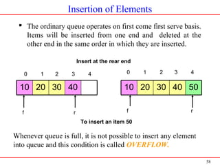
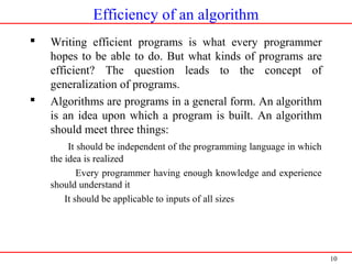
![59
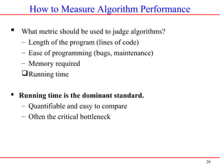
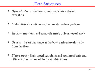
Function to insert an item at the rear end of the queue
void insert_rear(int item,int q[],int *r)
{
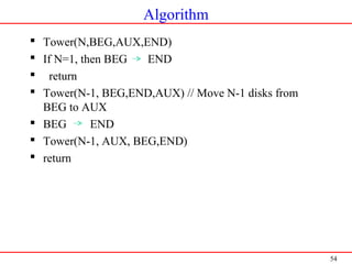
if(q_full(*r)) /* Is queue full */
{
printf(“Queue overflown”);
return;
}
/* Queue is not full */
q[++(*r)] = item;
}
int q_full(int r)
{
return (r == QUEUE_SIZE -1)? 1 : 0;
}](https://image.slidesharecdn.com/introductiontodatastructures-140603122653-phpapp02/85/Introduction-to-data-structures-and-Algorithm-59-320.jpg)
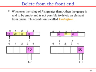
![61
Function to delete an item from the front end
void delete_front(int q[], int *f, int *r) {
if( q_empty(f , r) ) /* Is queue empty*/
{
printf(“Queue underflown”);
return;
}
printf(“The element deleted is %dn”,q[(*f)++]);
if( f > r )
{
f = 0;
r = -1;
}
}
int q_empty(int f,int r)
{
return (f>r) ? 1 : 0;
}](https://image.slidesharecdn.com/introductiontodatastructures-140603122653-phpapp02/85/Introduction-to-data-structures-and-Algorithm-61-320.jpg)
![62
Function to display the contents of queue
The contents of queue can be displayed only if queue is not empty. If
queue is empty an appropriate message is displayed.
void display(int q[], int f, int r)
{
int i;
if( q_empty (f , r )) /* Is queue empty*/
{
printf(“Queue is emptyn”);
return;
}
printf(“Contents of queue is n”);
for(i = f;i <=r;i++)
printf(“%dn”,q[i]);
}](https://image.slidesharecdn.com/introductiontodatastructures-140603122653-phpapp02/85/Introduction-to-data-structures-and-Algorithm-62-320.jpg)
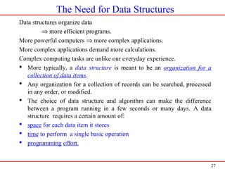
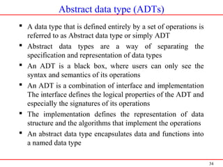
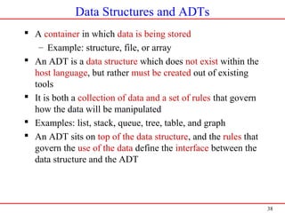
![64
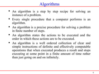
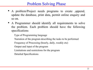
Insert at the front end
0 1 2 3 4
r
f
if(f==0 && r == -1)
q[++r] = item;
4030
0 1 2 3 4
f r
40302010
0 1 2 3 4
f r
if( f != 0)
q[--f] = item;
Not possible to insert
an item at the front end](https://image.slidesharecdn.com/introductiontodatastructures-140603122653-phpapp02/85/Introduction-to-data-structures-and-Algorithm-64-320.jpg)
![65
Function to insert an item at front end
void insert_front(int item,int q[],int *f,int *r)
{
if(*f == 0 && *r == -1)
{
q[++(*r)] = item;
return;
}
if(*f != 0)
{
q[--(*f)] = item;
return;
}
printf(“Front insertion not possible”);
}](https://image.slidesharecdn.com/introductiontodatastructures-140603122653-phpapp02/85/Introduction-to-data-structures-and-Algorithm-65-320.jpg)
![66
Function to delete an item from the rear end
void delete_rear(int q[], int *f,int *r)
{
if(q_empty(f, r))
{
printf(“Queue underflown”);
return;
}
printf(“The element deleted is %d”,q[(*r)--]);
if(f > r)
{
f = 0;
r = -1;
}
}](https://image.slidesharecdn.com/introductiontodatastructures-140603122653-phpapp02/85/Introduction-to-data-structures-and-Algorithm-66-320.jpg)
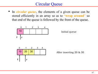
![69
Operations Performed on Circular Queues
Insert rear
Delete front
Display the contents of Queue
Function to insert an item at the rear end
void insert_rear(int item,int q[],int *r,int *count)
{
if(q_full(*count))
{
printf(“Overflow of Queuen”);
return;
}
r = (*r + 1) % QUEUE_SIZE; /* Increment rear pointer */
q[*r]=item; /* Insert the item */
*count +=1; /* Update the counter */
}
int(q_full(int count))
{
/* Return true if Q is full,else false */
return (count == QUEUE_SIZE - 1) ? 1 : 0;
}](https://image.slidesharecdn.com/introductiontodatastructures-140603122653-phpapp02/85/Introduction-to-data-structures-and-Algorithm-69-320.jpg)
![70
Function to delete an item from the front end
void delete_front(int q[], int *f, int *count)
{
if(q_empty(*count))
{
printf(“Underflow of queuen”);
return;
}
/* Access the item */
printf(“The deleted element is %dn”,q[*f]);
/* Point to next first item */
f = (*f + 1) % QUEUE_SIZE;
/* Update counter */
*count -= 1;
}
int(q_empty(int count))
{
/* Return true if Q is empty ,else false */
return(count == 0) ? 1 : 0;
}](https://image.slidesharecdn.com/introductiontodatastructures-140603122653-phpapp02/85/Introduction-to-data-structures-and-Algorithm-70-320.jpg)
![72
Function to insert an item at the correct place in priority queue.
void insert_item(int item,int q[], int *r)
{
int j;
if(q_full(*r))
{
printf(“Queue is fulln”);
return;
}
j = *r; /* Compare from this initial point */
/* Find the appropriate position */
while(j >= 0 && item < q[j])
{
q[j+1] = q[j]; /*Move the item at q[j] to its next position */
j--;
}
/* Insert an item at the appropriate position */
q[j+1]=item;
/* Update the rear item */
*r = *r + 1;
}](https://image.slidesharecdn.com/introductiontodatastructures-140603122653-phpapp02/85/Introduction-to-data-structures-and-Algorithm-72-320.jpg)

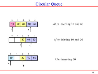
This document provides an introduction to data structures and algorithms. It discusses key concepts like algorithms, abstract data types (ADTs), data structures, time complexity, and space complexity. It describes common data structures like stacks, queues, linked lists, trees, and graphs. It also covers different ways to classify data structures, the process for selecting an appropriate data structure, and how abstract data types encapsulate both data and functions. The document aims to explain fundamental concepts related to organizing and manipulating data efficiently.