Download as PDF, PPTX
![Arrays
Prof. K. Adisesha (Ph. D)
13
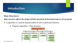
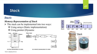
Arrays:
An array is defined as a set of finite number of homogeneous elements or same data
items:
➢ Declaration of array is as follows:
➢ Syntax: Datatype Array_Name [Size];
➢ Example: int arr[10];
✓ Where int specifies the data type or type of elements arrays stores.
✓ “arr” is the name of array & the number specified inside the square brackets is the
number of elements an array can store, this is also called sized or length of array.](https://image.slidesharecdn.com/datastructure-201021140600/85/Data-Structures-13-320.jpg)
![Arrays
Prof. K. Adisesha (Ph. D)
14
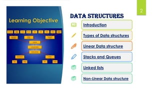
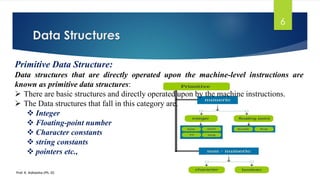
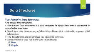
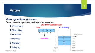
Arrays:
Represent a Linear Array in memory:
➢ The elements of linear array are stored in consecutive memory locations.
➢ It is shown below:
int A[5]={23, 4, 6, 15, 5, 7}](https://image.slidesharecdn.com/datastructure-201021140600/85/Data-Structures-14-320.jpg)
![Arrays
Prof. K. Adisesha (Ph. D)
15
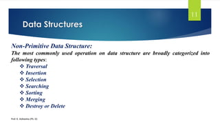
Calculating the length of the array:
The elements of array will always be stored in the consecutive (continues) memory
location.
➢ The number of elements that can be stored in an array, that is the size of array or its length is
given by the following equation:
o A[n] is the array size or length of n elements.
o The length of the array can be calculated by:
L = UB – LB + 1
o To Calculate the address of any element in array:
Loc(A[P])=Base(A)+W(P-LB)
o Here, UB is the largest Index and LB is the smallest index
➢ Example: If an array A has values 10, 20, 30, 40, 50, stored in location 0,1, 2, 3, 4 the UB = 4
and LB=0 Size of the array L = 4 – 0 + 1 = 5](https://image.slidesharecdn.com/datastructure-201021140600/85/Data-Structures-15-320.jpg)
![Arrays
Prof. K. Adisesha (Ph. D)
16
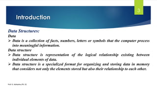
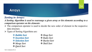
Types of Arrays:
The elements of array will always be stored in the consecutive (continues) memory
location. The various types of Arrays are:
➢ Single Dimension Array:
❖ Array with one subscript
❖ Ex: int A[i];
➢ Two Dimension Array
❖ Array with two subscripts (Rows and Column)
❖ Ex: int A[i][j];
➢ Multi Dimension Array:
❖ Array with Multiple subscripts
❖ Ex: int A[i][j]..[n];](https://image.slidesharecdn.com/datastructure-201021140600/85/Data-Structures-16-320.jpg)
![Arrays
Prof. K. Adisesha (Ph. D)
18
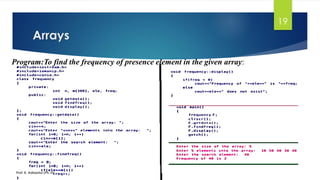
Traversing Arrays:
Traversing: It is used to access each data item exactly once so that it can be processed:
➢ We have linear array A as below:
1 2 3 4 5
10 20 30 40 50
➢ Here we will start from beginning and will go till last element and during this process
we will access value of each element exactly once as below:
A [0] = 10
A [1] = 20
A [2] = 30
A [3] = 40
A [4] = 50](https://image.slidesharecdn.com/datastructure-201021140600/85/Data-Structures-18-320.jpg)
![Arrays
Prof. K. Adisesha (Ph. D)
21
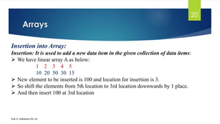
Insertion into Array:
Insertion into Array:
➢ Insertion 100 into Array
at Pos=3
A [0] = 10
A [1] = 20
A [2] = 50
A [3] = 30
A [4] = 15](https://image.slidesharecdn.com/datastructure-201021140600/85/Data-Structures-21-320.jpg)
![Arrays
Prof. K. Adisesha (Ph. D)
22
Insertion into Array: Add a new data item in the given array of data:
Insertion into Array:
A [0] = 10
A [1] = 20
A [2] = 50
A [3] = 30
A [4] = 15](https://image.slidesharecdn.com/datastructure-201021140600/85/Data-Structures-22-320.jpg)
![Arrays
Prof. K. Adisesha (Ph. D)
23
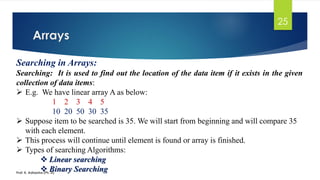
Deletion from Array:
Deletion: It is used to delete an existing data item from the given collection of data
items:
➢ Deletion 30 from Array
at Pos 3
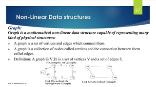
A [0] = 10
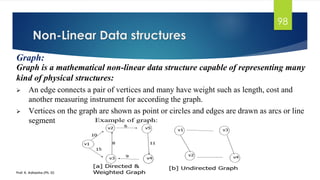
A [1] = 20
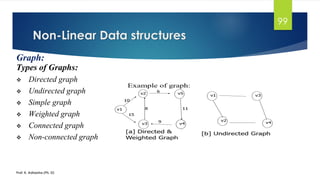
A [2] = 30
A [3] = 40
A [4] = 50](https://image.slidesharecdn.com/datastructure-201021140600/85/Data-Structures-23-320.jpg)
![Arrays
Prof. K. Adisesha (Ph. D)
24
Deletion from Array:
A [0] = 10
A [1] = 20
A [2] = 30
A [3] = 40
A [4] = 50](https://image.slidesharecdn.com/datastructure-201021140600/85/Data-Structures-24-320.jpg)
![Arrays
Prof. K. Adisesha (Ph. D)
38
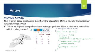
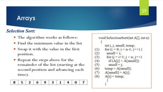
Insertion Sorting: ALGORITHM: Insertion Sort (A, N) A is an array with N unsorted elements.
◼ Step 1: for I=1 to N-1
◼ Step 2: J = I
While(J >= 1)
if ( A[J] < A[J-1] ) then
Temp = A[J];
A[J] = A[J-1];
A[J-1] = Temp;
[End if]
J = J-1
[End of While loop]
[End of For loop]
◼ Step 3: Exit](https://image.slidesharecdn.com/datastructure-201021140600/85/Data-Structures-38-320.jpg)
![Arrays
Prof. K. Adisesha (Ph. D)
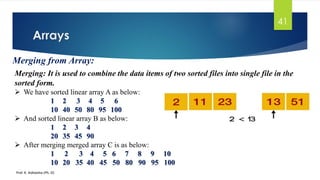
42
Two dimensional array:
A two dimensional array is a collection of elements and each element is identified by a
pair of subscripts. ( A[3] [3] ).
➢ The elements are stored in continuous memory locations.
➢ The elements of two-dimensional array as rows and columns.
➢ The number of rows and columns in a matrix is called as the order of the matrix and
denoted as MxN.
➢ The number of elements can be obtained by multiplying number of rows and number of
columns. A[0] A[1] A[2]
A[0] 10 20 30
A[1] 40 50 60
A[2] 70 80 90](https://image.slidesharecdn.com/datastructure-201021140600/85/Data-Structures-42-320.jpg)
![Arrays
Prof. K. Adisesha (Ph. D)
43
Representation of Two Dimensional Array:
A two dimensional array is a collection of elements and each element is identified by a
pair of subscripts. ( A[m] [n] )
➢ A is the array of order m x n. To store m*n number of elements, we need m*n memory
locations.
➢ The elements should be in contiguous memory locations.
➢ There are two methods:
❖ Row-major method
❖ Column-major method
A[0] A[1] A[2]
A[0] 10 20 30
A[1] 40 50 60
A[2] 70 80 90](https://image.slidesharecdn.com/datastructure-201021140600/85/Data-Structures-43-320.jpg)
![Arrays
Prof. K. Adisesha (Ph. D)
44
Representation of Two Dimensional Array:
Row-Major Method:
➢ All the first-row elements are stored in sequential
memory locations and then all the second-row
elements are stored and so on. Ex: A[Row][Col]
Column-Major Method:
➢ All the first column elements are stored in sequential
memory locations and then all the second-column
elements are stored and so on. Ex: A [Col][Row]
1000 10 A[0][0]
1002 20 A[0][1]
1004 30 A[0][2]
1006 40 A[1][0]
1008 50 A[1][1]
1010 60 A[1][2]
1012 70 A[2][0]
1014 80 A[2][1]
1016 90 A[2][2]
1000 10 A[0][0]
1002 40 A[1][0]
1004 70 A[2][0]
1006 20 A[0][1]
1008 50 A[1][1]
1010 80 A[2][1]
1012 30 A[0][2]
1014 60 A[1][2]
1016 90 A[2][2]
Row-Major Method
Col-Major Method](https://image.slidesharecdn.com/datastructure-201021140600/85/Data-Structures-44-320.jpg)
![Arrays
Prof. K. Adisesha (Ph. D)
45
Calculating the length of the 2D-Array
:A two dimensional array is a collection of elements and each element is identified by a
pair of subscripts. ( A[m] [n] )
➢ The size of array or its length is given by the following equation:
A[i][j] is the array size or length of m*n elements.
➢ To Calculate the address of i*j th element in array:
❖ Row-Major Method: Loc(A[i][j])=Base(A)+W[n(i-LB)+(j-LB)]
❖ Col-Major Method: Loc(A[i][j])=Base(A)+W[(i-LB)+m(j-LB)]
Here, W is the number of words per memory location and LB is the smallest index](https://image.slidesharecdn.com/datastructure-201021140600/85/Data-Structures-45-320.jpg)
![Arrays
Prof. K. Adisesha (Ph. D)
46
Advantages of Array
:A two dimensional array is a collection of elements and each element is identified by a
pair of subscripts. ( A[m] [n] )
➢ It is used to represent multiple data items of same type by using single name.
➢ It can be used to implement other data structures like linked lists, stacks, queues, tree,
graphs etc.
➢ Two-dimensional arrays are used to represent matrices.
➢ Many databases include one-dimensional arrays whose elements are records.](https://image.slidesharecdn.com/datastructure-201021140600/85/Data-Structures-46-320.jpg)
![Arrays
Prof. K. Adisesha (Ph. D)
47
Disadvantages of Array
:A two dimensional array is a collection of elements and each element is identified by a
pair of subscripts. ( A[m] [n] )
➢ We must know in advance the how many elements are to be stored in array.
➢ Array is static structure. It means that array is of fixed size. The memory which is
allocated to array cannot be increased or decreased.
➢ Array is fixed size; if we allocate more memory than requirement then the memory
space will be wasted.
➢ The elements of array are stored in consecutive memory locations. So insertion and
deletion are very difficult and time consuming.](https://image.slidesharecdn.com/datastructure-201021140600/85/Data-Structures-47-320.jpg)
![Stack
Prof. K. Adisesha (Ph. D)
52
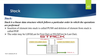
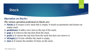
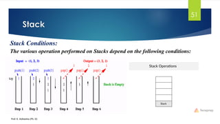
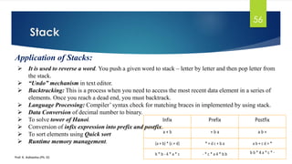
PUSH Operation:
The process of adding one element or item to the stack is represented by an operation
called as the PUSH operation:
ALGORITHM:
PUSH (STACK, TOP, SIZE, ITEM)
STACK is the array with N elements. TOP is the pointer to the top of the element of the array. ITEM to be inserted.
Step 1: if TOP = N then [Check Overflow]
PRINT “ STACK is Full or Overflow”
Exit
[End if]
Step 2: TOP = TOP + 1 [Increment the TOP]
Step 3: STACK[TOP] = ITEM [Insert the ITEM]
Step 4: Return](https://image.slidesharecdn.com/datastructure-201021140600/85/Data-Structures-52-320.jpg)
![ALGORITHM: POP (STACK, TOP, ITEM)
STACK is the array with N elements. TOP is the pointer to the top of the element of the array. ITEM
to be DELETED.
Step 1: if TOP = 0 then [Check Underflow]
PRINT “ STACK is Empty or Underflow”
Exit
[End if]
Step 2: ITEM = STACK[TOP] [copy the TOP Element]
Step 3: TOP = TOP - 1 [Decrement the TOP]
Step 4: Return
Stack
Prof. K. Adisesha (Ph. D)
54
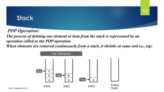
POP Operation:
The process of deleting one element or item from the stack is represented by an
operation called as the POP operation.](https://image.slidesharecdn.com/datastructure-201021140600/85/Data-Structures-54-320.jpg)
![Stack
Prof. K. Adisesha (Ph. D)
55
PEEK Operation:
The process of returning the top item from the stack but does not remove it called as the
PEEK operation.
ALGORITHM: PEEK (STACK, TOP)
STACK is the array with N elements. TOP is the pointer to the top of the element of the
array.
Step 1: if TOP = NULL then [Check Underflow]
PRINT “ STACK is Empty or Underflow”
Exit
[End if]
Step 2: Return (STACK[TOP] [Return the top element of the stack]
Step 3:Exit](https://image.slidesharecdn.com/datastructure-201021140600/85/Data-Structures-55-320.jpg)
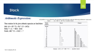
![An expression is a combination of operands and operators that after evaluation results
in a single value.
◼ Operand consists of constants and variables.
◼ Operators consists of {, +, -, *, /, ), ] etc.
➢ Expression can be
❖ Infix Expression: If an operator is in between two operands, it is called infix expression.
✓ Example: a + b, where a and b are operands and + is an operator.
❖ Postfix Expression: If an operator follows the two operands, it is called postfix expression.
✓ Example: ab +
❖ Prefix Expression: an operator precedes the two operands, it is called prefix expression.
✓ Example: +ab
Stack
Prof. K. Adisesha (Ph. D)
57
Arithmetic Expression:](https://image.slidesharecdn.com/datastructure-201021140600/85/Data-Structures-57-320.jpg)
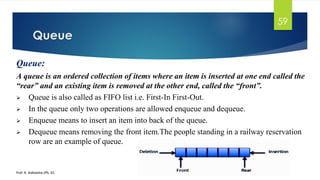
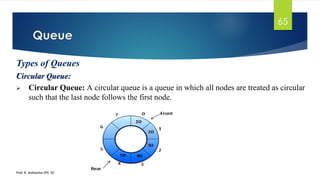
![Queue
Prof. K. Adisesha (Ph. D)
69
Queue Insertion Operation (ENQUEUE):
ALGORITHM: ENQUEUE (QUEUE, REAR, FRONT, ITEM)
QUEUE is the array with N elements. FRONT is the pointer that contains the location of the element to be deleted
and REAR contains the location of the inserted element. ITEM is the element to be inserted.
Step 1: if REAR = N-1 then [Check Overflow] Front Rear
PRINT “QUEUE is Full or Overflow”
Exit
[End if]
Step 2: if FRONT = NULL then [Check Whether Queue is empty]
FRONT = -1
REAR = -1
else
REAR = REAR + 1 [Increment REAR Pointer]
Step 3: QUEUE[REAR] = ITEM [Copy ITEM to REAR position]
Step 4: Return](https://image.slidesharecdn.com/datastructure-201021140600/85/Data-Structures-69-320.jpg)
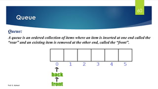
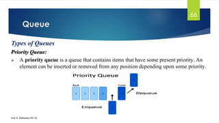
![Queue
Prof. K. Adisesha (Ph. D)
70
Queue Deletion Operation (DEQUEUE):
ALGORITHM: DEQUEUE (QUEUE, REAR, FRONT, ITEM)
QUEUE is the array with N elements. FRONT is the pointer that contains the location of the element to be deleted and REAR
contains the location of the inserted element. ITEM is the element to be inserted.
Step 1: if FRONT = NULL then [Check Whether Queue is empty] Front Rear
PRINT “QUEUE is Empty or Underflow”
Exit
[End if]
Step 2: ITEM = QUEUE[FRONT]
Step 3: if FRONT = REAR then [if QUEUE has only one element]
FRONT = NULL
REAR = NULL
else
FRONT = FRONT + 1 [Increment FRONT pointer]
Step 4: Return](https://image.slidesharecdn.com/datastructure-201021140600/85/Data-Structures-70-320.jpg)

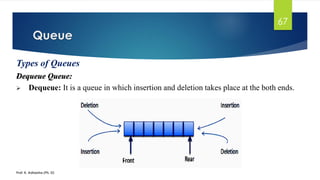
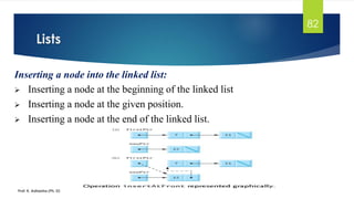
![Lists
Prof. K. Adisesha (Ph. D)
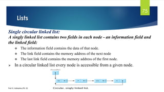
80
Operator new and delete:
The nodes of a linked list can be created by the following structure declaration:
➢ Operators new allocate memory space
➢ Operators new [ ] allocates memory space for array.
➢ Operators delete deallocate memory space.
➢ Operators delete [ ] deallocate memory space for array.
struct Node
{
int information;
struct Node *link;
}*node1, *node2;](https://image.slidesharecdn.com/datastructure-201021140600/85/Data-Structures-80-320.jpg)
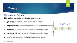
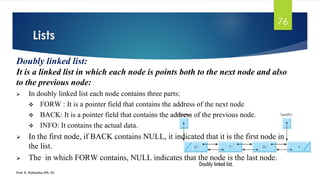
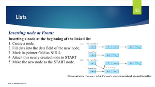
![81
Traversing is the process of accessing each node of the linked list exactly once to
perform some operation.
ALGORITHM: TRAVERS (START, P)
START contains the address of the first node. Another pointer p is temporarily used to visit all the nodes
from the beginning to the end of the linked list.
Step 1: P = START
Step 2: while P != NULL
Step 3: PROCESS data (P) [Fetch the data]
Step 4: P = link(P) [Advance P to next node]
Step 5: End of while
Step 6: Return
Traversing a linked list
Prof. K. Adisesha (Ph. D)](https://image.slidesharecdn.com/datastructure-201021140600/85/Data-Structures-81-320.jpg)
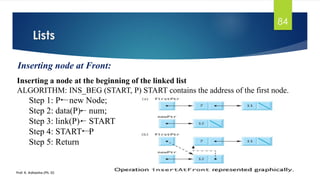
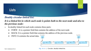
![ALGORITHM: INS_END (START, P)
START contains the address of the first node.
Step 1: START
Step 2: P START [identify the last node]
while P!= null
P next (P)
End while
Step 3: N new Node;
Step 4: data(N) item;
Step 5: link(N) null
Step 6: link(P) N
Step 7: Return
86
Inserting node at End
Prof. K. Adisesha (Ph. D)](https://image.slidesharecdn.com/datastructure-201021140600/85/Data-Structures-86-320.jpg)
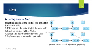
![87
Inserting node at a given Position
ALGORITHM: INS_POS (START, P1, P2)
START contains the address of the first node. P2 is new node
Step 1: START
Step 2: P1 START [Initialize node]
Count 0
Step 3: while P!= null
count count+1
P1 next (P1)
End while
Step 4: if (POS=1)
Call function INS_BEG( )
else if (POS=Count +1)
Call function INS_END( )
else if (POS<=Count)
P1 Start
For(i=1; i<=pos; i++)
P1 next(P1);
end for
[create] P2 new node
data(P2) item;
link(P2) link(P1)
link(P1) P2
else
PRINT “Invalid position”
Step 5: Return
Prof. K. Adisesha (Ph. D)](https://image.slidesharecdn.com/datastructure-201021140600/85/Data-Structures-87-320.jpg)
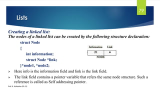
![Step 1: START
Step 2: P1 START [Initialize node]
Count 0
Step 3: while P!= null
count count+1
P1 next (P1)
End while
Step 4: if (POS=1)
Call function DEL_BEG( )
else if (POS=Count)
Call function DEL_END( )
else if (POS<=Count)
P2 Start
For(i=1; i<=pos; i++)
P1 P2
P2 link(P2)
end for
PRINT data(P2)
link(P1) link( P2)
free(P2)
End if
Step 5: Return
92
Deleting node at a given Position
ALGORITHM: DEL_POS (START, P1, P2)
START contains the address of the first node. P2 is DEL-node
Prof. K. Adisesha (Ph. D)](https://image.slidesharecdn.com/datastructure-201021140600/85/Data-Structures-92-320.jpg)
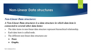
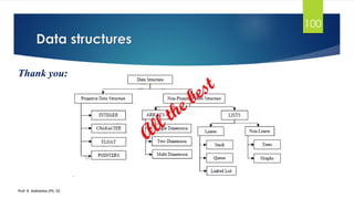

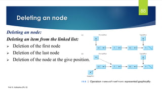
The document discusses data structures and arrays. It begins by defining data, data structures, and how data structures affect program design. It then categorizes data structures as primitive and non-primitive. Linear and non-linear data structures are described as examples of non-primitive structures. The document focuses on arrays as a linear data structure, covering array declaration, representation in memory, calculating size, types of arrays, and basic operations like traversing, searching, inserting, deleting and sorting. Two-dimensional arrays are also introduced.