Chapter 09 design and analysis of algorithms

CHAPTER - 09
DESIGN AND ANALYSIS OF ALGORITHMS

Unit I
Programming and Computational
Thinking (PCT-2)
(80 Theory + 70 Practical)
DCSc & Engg, PGDCA,ADCA,MCA.MSc(IT),Mtech(IT),MPhil (Comp. Sci)
Department of Computer Science, Sainik School Amaravathinagar
Cell No: 9431453730
Praveen M Jigajinni
Prepared by
Courtesy CBSE
Class XII

INTRODUCTION
What is an Algorithm?
• An algorithm is a step-by-step procedure
for solving a problem in a finite amount of time.
The word algorithm comes from the name of a
Persian mathematician Abu Ja’far Mohammed ibn-i
Musa al Khowarizmi. For a given problem,
o There can be more than one solution (more than
one algorithm) .
o An algorithm can be implemented using different
programming languages on different platforms.

MUHAMMAD IBN MUSA AL-KHWARIZMI
Muḥammad ibn Mūsā al-
Khwārizmī (Persian: ‫محمد‬‫بن‬‫موسى‬
‫;خوارزمی‬ c. 780 – c. 850),
Formerly Latinized as Algoritmi, was
a Persian scholar who produced
works in mathematics, astronomy,
& geography under the patronage
of the Caliph Al-Ma'mun of
the Abbasid Caliphate.
Around 820 AD he was appointed as the astronomer
and head of the library of the House of
Wisdom in Baghdad.

What is Design of an Algorithm?
Design of an algorithm is an area of
computer science which minimizes the cost.
Always design algorithms which minimize
the cost.
DESIGN OF ALGORITHM

What is an Analysis of Algorithm?
• Analysis of Algorithms is the area of
computer science that provides tools to analyze
the efficiency of different methods of solutions.
In short predict the cost of an algorithm in
terms of resources and performance is called
analysis of Algorithm.
ANALYSIS ALGORITHM

WHAT IS PROGRAM?
A program is the expression of an
algorithm in a programming language.
Sometimes works such as procedure, function
and subroutine are used synonymously
program.

PROPERTIES OF ALGORITHM
Donald Ervin Knuth has given a list of five
properties for an algorithm, these
properties are:
1) FINITENESS
2) DEFINITENESS
3) INPUT
4) OUTPUT
5) EFFECTIVENESS

1) FINITENESS:
An algorithm must always terminate
after a finite number of steps. It
means after every step one reach
closer to solution of the problem and
after a finite number of steps
algorithm reaches to an end point.

2) DEFINITENESS
Each step of an algorithm must be
precisely defined. It is done by well
thought actions to be performed at
each step of the algorithm. Also the
actions are defined unambiguously for
each activity in the algorithm.

3) INPUT
Any operation you perform need
some beginning value/quantities
associated with different activities in
the operation. So the value/quantities
are given to the algorithm before it
begins.

4) OUTPUT:
One always expects output/result
(expected value/quantities) in terms of output
from an algorithm. The result may be obtained
at different stages of the algorithm. If some
result is from the intermediate stage of the
operation then it is known as intermediate
result and result obtained at the end of
algorithm is known as end result. The output
is expected value/quantities always have a
specified relation to the inputs.

5) EFFECTIVENESS:
Algorithms to be developed/written
using basic operations. Actually operations
should be basic, so that even they can in
principle be done exactly and in a finite
amount of time by a person, by using paper
and pencil only.

WHY STUDY ALGORITHMS AND PERFORMANCE?

WHY STUDY ALGORITHMS AND PERFORMANCE?
• Algorithms help us to understand scalability.
• Performance often draws the line between
what is feasible and what is impossible.
• Algorithmic mathematics provides a language
for talking about program behavior.
• The lessons of program performance generalize
to other computing resources.
• Speed is fun!

EXAMPLE
Given problem may have number of solutions
for example:
Eating Apple is the given problem
Solution 1:
1. Wash the Apple.
2. Cut the Apple in to pieces.
3. Eat Apple.

EXAMPLE
for example:
Solution 2:
1. Wash the Apple.
2. Prepare a custard Apple.
3. Eat it.

EXAMPLE
for example:
Solution 3:
1. Wash the Apple.
2. Make Juice of it.
3. Drink the Juice.

EXAMPLE
for example:
Solution 4:
1. Wash the Apple.
2. Mix it with other Fruits (salad).
3. Eat it.

PROBLEM SOLVING
In computer science problem can be solved in n
number of ways
PROBLEM P1
Solution S1 Solution S2
Solution S3 Solution S4

PROBLEM SOLVING
Factorial of a number
Writing Non
Recursive
Function
Writing
Recursive
Function
In computer science problem can be solved in n
number of ways

Factorial of a number - Non Recursive Function

Factorial of a number - Non Recursive Function
OUTPUT

Factorial of a number - Recursive Function

Factorial of a number - Recursive Function
OUTPUT

ALGORITHM / PROGRAM EFFICIENCY

BETTER ALGORITHM/PROGRAM
One can say a program or an algorithm better
one, which exhibits following characteristics
1. Less Line of Code
2. Takes Less Space
3. Easier to Understand
4. Less Statement to execute.
5. Looks more beautiful.

PROGRAM EFFICIENCY
There aspects of algorithmic performance:
1. Less Line of Code: It is not correct matrix
to measure the better program.
This can not be the primary measure to check
the efficiency of the code.
When a program is written in HLL it has to
undergo following stages before it is being executed
Contd..

PROGRAM EFFICIENCY
HLL PREPROCESSOR COMPILER
ASSEMBLER
LOADER / LINKER
Executable Code
PREPROCESSOR
Generates Pure HLL
COMPLIER Generates
ASSEMBLY CODE
ASSEMBLER Generates
MACHINE CODE
LOADER / LINKER
Generates Exe CODE

PROGRAM EFFICIENCY
2. Takes Less Space: Less space can be of
a) Program file size : Once a program is written
that is stored under a file. That file occupies some
space in the memory us called program file size or
simply file size.
b) Execution space or Process Space Or Space
Complexity : During execution system allots memory
for the variables constants and function calls this
space is called as Execution space or process space
or Space Complexity – It is the one which is
measures the efficiency of the program.

PROGRAM EFFICIENCY
3. Easier to Understand : Nothing to do with the
execution of the program, hence it is not the
criteria for the assess the program efficiency.
4. Less Statement to execute : if a program
executes minimum instruction to get a
desired results then it is said to be less
Statement execution time it also called as
Time Complexity, which is the another
criteria for measuring the program efficiency.

PROGRAM EFFICIENCY
5. Looks more elegant: A program may look
elegant by its indentation and proper usage
of comments but it has nothing to do with
the program efficiency and this point stands
invalid.

There are two aspects of algorithmic
performance or efficiency:
• Time
• Instructions take time.
• How fast does the algorithm perform?
• What affects its runtime?
• Space
• Data structures take space
• What kind of data structures can be used?
• How does choice of data structure affect the
runtime?
ALGORITHM / PROGRAM EFFICIENCY

PROGRAM EFFICIENCY
Now, We can understand an efficient
algorithm or program. The efficiency is
measured by:
1. TIME COMPLEXITY
2. SPACE COMPLEXITY

1. TIME COMPLEXITY
What is Time Complexity?
In computer science, the time
complexity is the computational
complexity that describes the amount
of time it takes to run an algorithm.
Time Complexity of algorithm/code
is not equal to the actual time required to
execute a particular code but the number of
times a statement executes.
Contd..

1. TIME COMPLEXITY
What is Time Complexity?
(ANOTHER DEFINITION)
Time complexity is a concept in computer
science that deals with the quantification of the
amount of time taken by a set of code or
algorithm to process or run as a function of the
amount of input.
In other words, time complexity is
essentially efficiency, or how long a program
function takes to process a given input.

2. SPACE COMPLEXITY
What is Space Complexity?
Space complexity in algorithm
development is a metric for how much storage
space the algorithm needs in relation to its
inputs. This measurement is extremely useful in
some kinds of programming evaluations as
engineers, coders and other scientists look at
how a particular algorithm works.
Contd..

2. SPACE COMPLEXITY
Space Complexity of an algorithm is total
space taken by the algorithm with respect to the
input size. Space complexity includes both
Auxiliary space and space used by input.

2. SPACE COMPLEXITY
(ANOTHER DEFINITION)
(Wikipedia definition) In computer
science, the space complexity of an algorithm
or a computer program is the amount of
memory space required to solve an instance
of the computational problem as a function
of the size of the input. It is the memory
required by an algorithm to execute a
program and produce output

Why performance analysis?
There are many important things that
should be taken care of when we write a
program, like user friendliness, modularity,
security, maintainability, etc. then why to worry
about performance?
The answer to this is simple, we can have
all the above things only if we have
performance.

Given two algorithms for a task, how do
we find out which one is better?
One naive way of doing this is –
implement both the algorithms and run the
two programs on your computer for different
inputs and see which one takes less time.
There are many problems with this approach
for analysis of algorithms.
1) It might be possible that for some inputs,
first algorithm performs better than the
second. And for some inputs second
performs better.

2) It might also be possible that for some
inputs, first algorithm perform better on
one machine and the second works better
on other machine for some other inputs.
Asymptotic Analysis is the big idea that
handles above issues in analyzing
algorithms. In Asymptotic Analysis, we
evaluate the performance of an algorithm
in terms of input size

Asymptotic Analysis
What is Asymptotic Analysis?
Asymptotic analysis of an algorithm
refers to defining the mathematical
boundation / framing of its run-time
performance. Using asymptotic analysis,
we can very well conclude the best case,
average case, and worst case scenario of an
algorithm.

KINDS OF ANALYSES
Usually, the time required by an
algorithm falls under three types −
Best Case − Minimum time required for
program execution.
Average Case − Average time required for
program execution.
Worst Case − Maximum time required for
program execution.

Asymptotic Notations
What is Asymptotic Notation?
Asymptotic Notations are the
expressions that are used to represent the
complexity of an algorithm.
OR
Asymptotic Notations provides with a
mechanism to calculate and represent time
and space complexity for any algorithm.

What is an order of growth or order of
growth of an algorithm?

Order of growth in algorithm means how
the time for computation increases when you
increase the input size. It really matters when
your input size is very large. Order of
growth provide only a crude description of the
behavior of a process.

How to compute Time Complexity or
Order of Growth of any program

Time Complexity gives us an idea of
running time of any program w.r.t. the size of
input fed to the program. Order of Growth is
just another word for Time Complexity.
We will go through some of basic and
most common time complexities such as:
How to compute Time Complexity or
Order of Growth of any program

Asymptotic Notations
Following are the commonly used
asymptotic notations to calculate the running
time complexity of an algorithm.
1. Ο Notation ( Big Oh Notation)
2. Ω Notation (Omega Notation)
3. θ Notation (Theta Notation)
Worst
Case
Best
Case
Avg
Case

Big O notation is used in Computer
Science to describe the performance or
complexity of an algorithm.
Big O specifically describes the
worst-case scenario, and can be used to
describe the execution time required or the
space used (e.g. in memory or on disk) by an
algorithm.
NOTE: O stands for Order of Growth

1. O(1)
printFirstElementOfList(lst1):
print("First element of
List =,lst1)
printFirstElementOfList(lst1)
This function runs in O(1) time (or "constant
time") relative to its input. The input array could be
1 item or 1,000 items, but this function would still
just require one step.

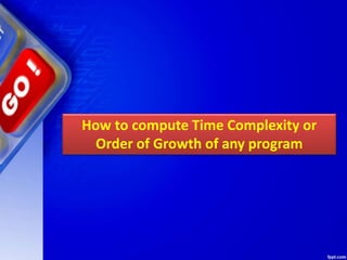
2. O(n)
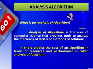
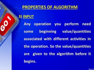
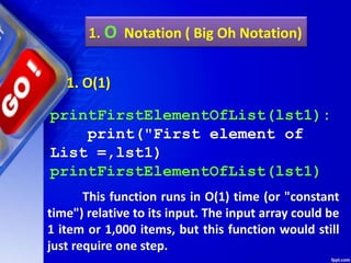
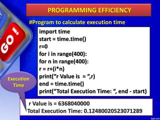
printAllElementOfArray(lst2, size):
for i in range(0,size):
print("n", lst2[i])
printAllElementOfArray(lst2, size)
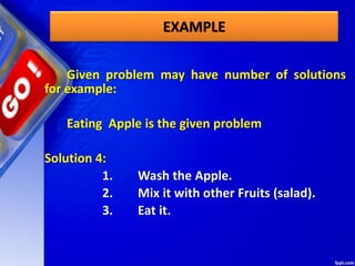
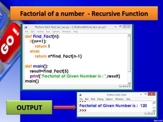
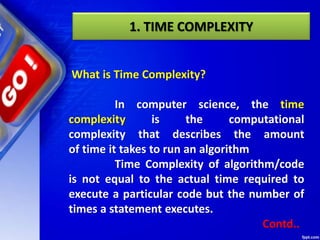
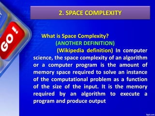
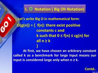
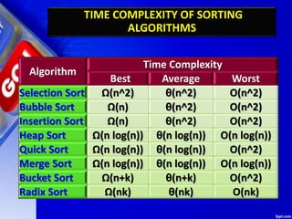
This function runs in O(n) time (or "linear
time"), where n is the number of items in the
array. If the array has 10 items, we have to print
10 times. If it has 1000 items, we have to print
1000 times.

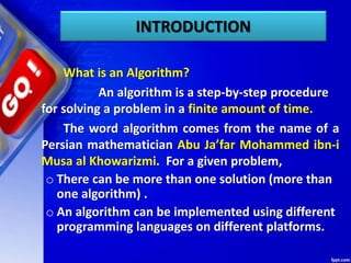
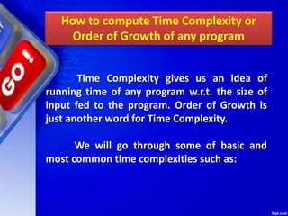
2. O(n)
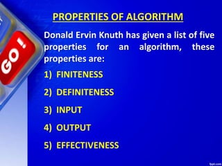
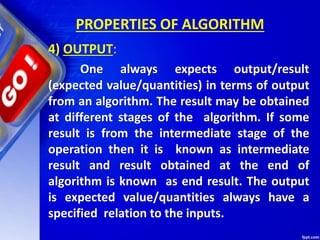
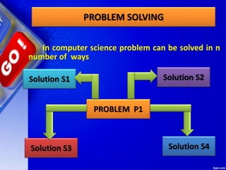
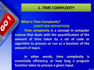
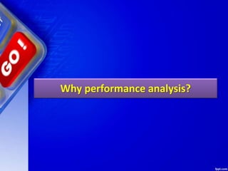
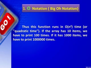
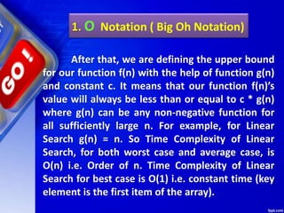
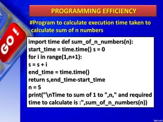
Here we're nesting two loops. If our array
has n items, our outer loop runs n times and our
inner loop runs n times for each iteration of the
outer loop, giving us n2 total prints.
printAllPossibleOrderedPairs(lis2,
size):
for i in range(0,size)
for j in range(0,size):
print("%n", lst2[i], lst2[j])

Thus this function runs in O(n2) time (or
"quadratic time"). If the array has 10 items, we
have to print 100 times. If it has 1000 items, we
have to print 1000000 times.

4. O(2n)
fibonacci(i num):
if (num <= 1): return num;
else:
return fibonacci(num - 2) + fibonacci(num - 1)
An example of an O(2n) function is the recursive
calculation of Fibonacci numbers. O(2n) denotes an
algorithm whose growth doubles with each addition to
the input data set. The growth curve of an O(2n) function
is exponential - starting off very shallow, then rising
meteorically.
1. Big Oh Notation - Ο

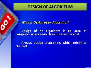
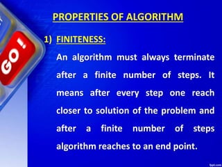
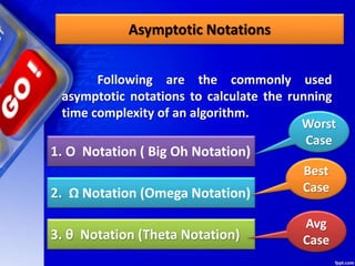
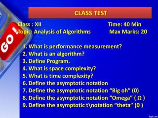
5. Drop the constants
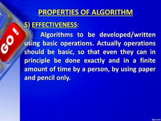
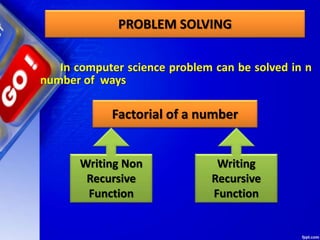
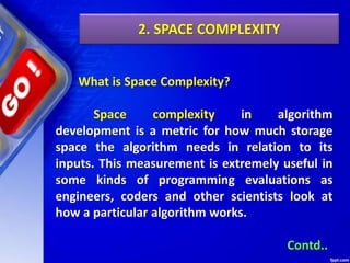
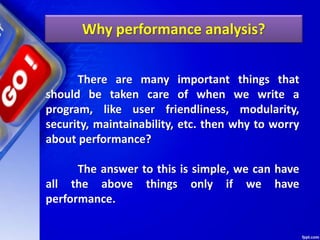
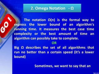
When you're calculating the big O
complexity of something, you just throw out the
constants. Like:
printAllItemsTwice(lst2,size):
print("n", lst2[i])
print(“n", lst2[i])
This is O(2n), which we just call O(n).

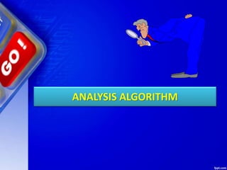
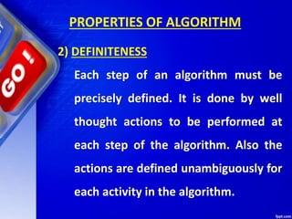
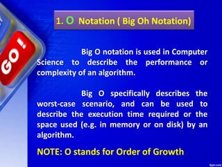
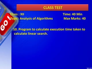
5. Drop the constants
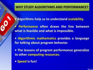
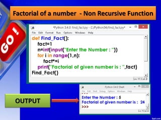
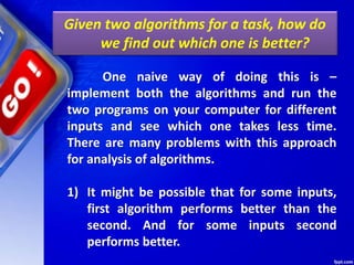
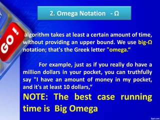
This is O(1 + n/2 + 100), which we just call O(n).
printlist(lst2,size):
print("First element =n",arr[0]);
for i in range(0, size/2):
print("%dn", arr[i]);
for i in range(0,100):
print("Hin")
printlist(lst2,size)
Remember, for big O notation we're looking at
what happens as n gets arbitrarily large. As n gets really
big, adding 100 or dividing by 2 has a decreasingly
significant effect.

6. Drop the less significant terms
printAllNumbersThenAllPairSums(lst2, size):
print(“n", lst2[i])
for j in range(0,size):
print("%dn", lst2[i] + lst2[j])
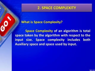
Here our runtime is O(n + n2), which we
just call O(n2).

Big O complexity can be visualized with this
graph:

Let’s write Big O in mathematical form:
O(g(n)) = { f(n): there exist positive
constants c and
k such that 0 ≤ f(n) ≤ cg(n) for
all n ≥ k
}
At first, we have chosen an arbitrary constant
called k as a benchmark for large input means our
input is considered large only when n ≥ k.
Contd..

After that, we are defining the upper bound
for our function f(n) with the help of function g(n)
and constant c. It means that our function f(n)’s
value will always be less than or equal to c * g(n)
where g(n) can be any non-negative function for
all sufficiently large n. For example, for Linear
Search g(n) = n. So Time Complexity of Linear
Search, for both worst case and average case, is
O(n) i.e. Order of n. Time Complexity of Linear
Search for best case is O(1) i.e. constant time (key
element is the first item of the array).

2. Omega Notation - Ω
The notation Ω(n) is the formal way to
express the lower bound of an algorithm's
running time. It measures the best case time
complexity or the best amount of time an
algorithm can possibly take to complete.
OR
Big Ω describes the set of all algorithms that
run no better than a certain speed (it’s a lower
bound)
Sometimes, we want to say that an

algorithm takes at least a certain amount of time,
without providing an upper bound. We use big-Ω
notation; that's the Greek letter "omega.“
For example, just as if you really do have a
million dollars in your pocket, you can truthfully
say "I have an amount of money in my pocket,
and it's at least 10 dollars,“
NOTE: The best case running
time is Big Omega

Let’s write Omega Ω in mathematical form:
For a given function g(n), we denote by
Ω(g(n)) the set of functions.
Ω (g(n)) = {f(n): there exist positive constants c
and n0 such that 0 <= c*g(n) <= f(n) for all n >=
n0}.
Best case performance of an algorithm is
generally not useful, the Omega notation is the
least used notation among all three.

3. Theta Notation - θ
The θ notation describes asymptotic tight bounds

3. Theta Notation - θ
You can use the big-Theta notation to
describe the average-case complexity. But you can
also use any other notation for this purpose. If an
algorithm has the average-casetime complexity of,
say, 3*n^2 - 5n + 13 , then it is true that
its average-case time complexity is Theta(n^2) ,
O(n^2) , and O(n^3)

TIME COMPLEXITY OF SORTING
ALGORITHMS

TIME COMPLEXITY OF SORTING
ALGORITHMS
Algorithm
Time Complexity
Best Average Worst
Selection Sort Ω(n^2) θ(n^2) O(n^2)
Bubble Sort Ω(n) θ(n^2) O(n^2)
Insertion Sort Ω(n) θ(n^2) O(n^2)
Heap Sort Ω(n log(n)) θ(n log(n)) O(n log(n))
Quick Sort Ω(n log(n)) θ(n log(n)) O(n^2)
Merge Sort Ω(n log(n)) θ(n log(n)) O(n log(n))
Bucket Sort Ω(n+k) θ(n+k) O(n^2)
Radix Sort Ω(nk) θ(nk) O(nk)

SPACE COMPLEXITY OF SEARCHING AND
SORTING ALGORITHMS

SPACE COMPLEXITY OF SEARCHING AND
SORTING ALGORITHMS
Algorithm Space complexity
Selection sort O(1)
Merge sort O(N)
Linear search O(1)
Binary search O(1)

TIME COMPLEXITY OF SEARCHING
ALGORITHMS

TIME COMPLEXITY OF SEARCHING ALGORITHMS
Algorithm Best case Average Worst case
Linear search O(1) O(N) O(N)
Binary search O(1) O(log N) O(log N)

PROGRAMMING EFFICIENCY
import time
start = time.time()
r=0
for i in range(400):
for n in range(400):
r = r+(i*n)
print(“r Value is = “,r)
end = time.time()
print(“Total Execution Time: “, end - start)
r Value is = 6368040000
Total Execution Time: 0.12480020523071289
#Program to calculate execution time
Execution
Time

PROGRAMMING EFFICIENCY
import time def sum_of_n_numbers(n):
start_time = time.time() s = 0
for i in range(1,n+1):
s = s + i
end_time = time.time()
return s,end_time-start_time
n = 5
print("nTime to sum of 1 to ",n," and required
time to calculate is :",sum_of_n_numbers(n))
#Program to calculate execution time taken to
calculate sum of n numbers

CLASS TEST
1. What is performance measurement?
2. What is an algorithm?
3. Define Program.
4. What is space complexity?
5. What is time complexity?
6. Define the asymptotic notation
7. Define the asymptotic notation “Big oh” (0)
8. Define the asymptotic notation “Omega” ( Ω )
9. Define the asymptotic tnotation “theta” (θ )
Class : XII Time: 40 Min
Topic: Analysis of Algorithms Max Marks: 20

CLASS TEST
10. Program to calculate execution time taken to
calculate linear search.
Class : XII Time: 40 Min
Topic: Analysis of Algorithms Max Marks: 40

Chapter 09 design and analysis of algorithms

Recommended

Recommended

More Related Content

What's hot

What's hot (20)

Similar to Chapter 09 design and analysis of algorithms

Similar to Chapter 09 design and analysis of algorithms (20)

More from Praveen M Jigajinni

More from Praveen M Jigajinni (20)

Recently uploaded

Recently uploaded (20)

Chapter 09 design and analysis of algorithms