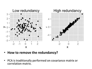
Dimensionality
Reduction
What is Dimensionality Reduction?
• In machine learning we are having too many factors on
which the final classification is done. These factors are
basically, known as variables.
• The higher the number of features, the harder it gets to
visualize the training set and then work on it.
• Sometimes, most of these features are correlated, and
hence redundant. This is where dimensionality reduction
algorithms come into play.
• We are generating a tremendous amount of data daily. In
fact, 90% of the data in the world has been generated in the
last 3-4 years! The numbers are truly mind boggling.
• Below are just some of the examples of the kind of data
being collected:
o Facebook collects data of what you like, share, post,
places you visit, restaurants you like, etc.
o Your smartphone apps collect a lot of personal
information about you
o Amazon collects data of what you buy, view, click, etc.
on their site
o Casinos keep a track of every move each customer
makes
o As data generation and collection keeps increasing,
visualizing it and drawing inferences becomes more and
more challenging.
• Let us understand this with a simple example. Consider the below image:
• Here we have weights of similar objects in Kg (X1) and Pound (X2). If we use both
of these variables, they will convey similar information. So, it would make sense
to use only one variable. We can convert the data from 2D (X1 and X2) to 1D (Y1)
as shown below:
• Similarly, we can reduce p dimensions of the data into a subset of k dimensions
(k<<n). This is called dimensionality reduction.
Components of Dimensionality Reduction
There are two components of dimensionality reduction:
Feature selection
• In this, we need to find a subset of the original set of variables. Also, need a
subset which we use to model the problem. This technique is used for
selecting the features which explain the most of the target variable(has a
correlation with the target variable).This test is ran just before the model is
applied on the data.
• To explain it better let us go by an example: there are 10 feature and 1
target variable, 9 features explain 90% of the target variable and 10 features
together explains 91% of the target variable. So the 1 variable is not making
much of a difference so you tend to remove that before modelling
• Selection of the features with the highest "importance"/influence on the
target variable, from a set of existing features. This can be done with
various techniques: e.g. Linear Regression, Decision Trees, calculation of
"importance" weights (e.g. Fisher score, ReliefF)
Feature Extraction
• We use this, to reduces the data in a high dimensional space
to a lower dimension space, i.e. a space with lesser no. of
dimensions.
• When you don't know anything about the data like no data
dictionary, too many features which means the data is not in
understandable format. Then you try applying this technique
to get some features which explains the most of the data.
Feature extraction involves a transformation of the features,
which often is not reversible because some information is
lost in the process of dimensionality reduction.
 You can apply Feature Extraction on the given data to extract
features and then apply Feature Selection with respect to the
Target Variable to select the subset which can help in making
a good model with good results.
Problems of Dimensionality
• Real world applications usually come with large number
of features – Text in documents is represented using
frequencies of tens of thousands of words – Images are
often represented by extracting local features from a
large number of regions within an image
• Naive intuition: more the number of features, the
better the classification performance? – Not always!
• There are two issues that must be confronted with high
dimensional feature spaces
– How does the classification accuracy depend on the
dimensionality and the number of training samples
– The computational complexity of designing a classifier
Increasing Dimensionality
Gives:
• If a given set of features does not result in
good performance, it is natural to add more
features
• High dimensionality results in increased cost
and complexity for both feature extraction
and classification .
Curse of Dimensionality
• In practice, increasing dimensionality beyond a certain
point in the presence of finite number of training
samples results in worse, rather than better
performance.
• For quick grasp, consider this example: Say, you
dropped a coin on a 100 meter line. How do you find
it? Simple, just walk on the line and search. But what if
it’s 100 x 100 sq. m. field? It’s already getting tough,
trying to search a (roughly) football ground for a single
coin. But what if it’s 100 x 100 x 100 cu.m space?! You
know, football ground now has thirty-story height.
Good luck finding a coin there! That, in essence is
“curse of dimensionality”.
Figure . As the dimensionality increases, the classifier’s
performance increases until the optimal number of
features is reached. Further increasing the dimensionality
without increasing the number of training samples results
in a decrease in classifier performance.
Curse of Dimensionality
• Solutions?
Dimensionality Reduction
- Problems arise when performing recognition in a
high-dimensional space (e.g., curse of
dimensionality).
- Significant improvements can be achieved by first
mapping the data into a lower-dimensionality
space.
Dimensional space Representation
• (1) Higher-dimensional space representation: x = a1v1 + a2v2 + ... +
aN vN v1 , v2 , ..., vN is a basis of the N-dimensional space
• (2) Lower-dimensional space representation: xˆ = b1u1 + b2u2 + ... +
bK uK u1 , u2 , ..., uK is a basis of the K-dimensional space
Why is Dimensionality Reduction required?
Here are some of the benefits of applying dimensionality reduction
to a dataset:
• Space required to store the data is reduced as the number of dimensions comes
down
• Less dimensions lead to less computation/training time
• Some algorithms do not perform well when we have a large dimensions. So
reducing these dimensions needs to happen for the algorithm to be useful.
• It takes care of multi collinearity by removing redundant features. For example,
you have two variables – ‘time spent on treadmill in minutes’ and ‘calories burnt’.
These variables are highly correlated as the more time you spend running on a
treadmill, the more calories you will burn. Hence, there is no point in storing
both as just one of them does what you require.
• It helps in visualizing data. As discussed earlier, it is very difficult to visualize data
in higher dimensions so reducing our space to 2D or 3D may allow us to plot and
observe patterns more clearly
Dimensionality Reduction Methods
for Feature Extraction
Dimensionality Reduction Methods
• The goal for any dimensional reduction method is to reduce the
dimensions of the original data for different purposes such as visualization,
decrease CPU time, ..etc..
• Dimensionality reduction techniques are important in many applications
related to machine learning, data mining, Bioinformatics,biometric and
information retrieval.
• There are following types of dimensionality reduction methods, namely,
supervised and unsupervised.
• PCA
• LDA
• Kernel PCA, etc..
First Method
Principal Component Analysis (PCA)
1. Principal Component Analysis (PCA)
• The main idea of principal component analysis (PCA) is to reduce the dimensionality
of a data set consisting of many variables correlated with each other, either heavily or
lightly, while retaining the variation present in the dataset, up to the maximum
extent.
• “The same is done by transforming the variables to a new set of variables (feature
extraction), which are known as the principal components (or simply, the PCs).”
Or
• “PCA reduces data by geometrically projecting them onto lower dimensions called
principal components (PCs), with the goal of finding the best summary of the data
using a limited number of PCs.”
• Principal Components Analysis (PCA) is arguably one of the most widely used
statistical methods. It has applications in nearly all areas of statistics and machine
learning including clustering, dimensionality reduction, face recognition, signal
processing, image compression, visualisation and prediction.
Let’s understand by an example
1. PCA & Genetics
• The human genome is an incredibly complex system. Our DNA has
approximately 3 billion base pairs, which are inherited from
generation to generation but which are also subject to random (and
not so random) mutation.
• As humans, we share 99.9% of our DNA - that's less than 0.1%
difference between all of us and only 1.5% difference between our
DNA and the DNA of chimpanzees.
• Despite these similarities, the differences in our DNA can be used to
uniquely identify every single one of us.
• There is an incredible amount of variability (both similarities and
dissimilarities) in our DNA - what is perhaps surprising initially, is
that this variability can be strongly linked to geography and it is
these geographical patterns which are picked up by prinicpal
components analysis.
Main purpose of PCA
The main goals of principal component analysis are:
• to identify hidden pattern in a data set
• to reduce the dimensionnality of the data by removing the noise
and redundancy in the data
• to identify correlated variables
• PCA method is particularly useful when the variables within the
data set are highly correlated.
• Correlation indicates that there is redundancy in the data. Due to
this redundancy, PCA can be used to reduce the original variables
into a smaller number of new variables ( = principal components)
explaining most of the variance in the original variables.
• How to remove the redundancy?
• PCA is traditionally performed on covariance matrix or
correlation matrix.
How PCA Works
• Broadly, there are probably two ways to use PCA: the first is simply
for dimensionality reduction, to take data in high dimensions and
create a reduced-representation as is the case with image
compression.
• The second, is to extract meaningful factors from high dimensional
data in a way that helps us interpret the major trends in our data, as
is the case with the genetics example above.
• I want to focus on the second case, being able to extract & explain
structure in your data. To understand the outputs of PCA it's
important to understand how it works.
• The key to PCA is that it exploits the variance of features (columns
in your data) as well as the covariance between features.
• PCA is traditionally performed on covariance matrix or correlation
matrix.
Covariance Matrix Method
• In this method, there are two main steps to
calculate the PCs of the PCA space.
1. The covariance matrix of the data matrix (X)
is calculated.
2. The eigenvalues and eigenvectors of the
covariance matrix are calculated.
• Covariance: A covariance matrix contains the
covariance's between all possible pairs of
variables in the data set
• Eigen values : The numbers on the diagonal of
the diagonaized covariance matrix are called
eigenvalues of the covariance matrix. Large
eigenvalues correspond to large variances.
• Eigenvectors : The directions of the new rotated
axes are called the eigenvectors of the covariance
matrix.
Steps for principal component analysis
• The procedure includes 5 simple steps :
1. Prepare the data :
• Center the data : subtract the mean from each variables. This produces a data set whose mean is
zero.
• Scale the data : If the variances of the variables in your data are significantly different, it’s a good
idea to scale the data to unit variance. This is achieved by dividing each variables by its standard
deviation.
2. Calculate the covariance/correlation matrix
3. Calculate the eigenvectors and the eigenvalues of the covariance matrix
4. Choose principal components : eigenvectors are ordered by eigenvalues from the highest to
the lowest. The number of chosen eigenvectors will be the number of dimensions of the new
data set. eigenvectors = (eig_1, eig_2,…, eig_n)
5. compute the new dataset :
• transpose eigeinvectors : rows are eigenvectors
• transpose the adjusted data (rows are variables and columns are individuals)
• new.data = eigenvectors.transposed X adjustedData.transposed
Disadvantages of Dimensionality Reduction
• Basically, it may lead to some amount of data
loss.
• Although, PCA tends to find linear correlations
between variables, which is sometimes
undesirable.
• Also, PCA fails in cases where mean and
covariance are not enough to define datasets.
• Further, we may not know how many principal
components to keep- in practice, some thumb
rules are applied.

PCA.pptx

  • 1.
  • 2.
    What is DimensionalityReduction? • In machine learning we are having too many factors on which the final classification is done. These factors are basically, known as variables. • The higher the number of features, the harder it gets to visualize the training set and then work on it. • Sometimes, most of these features are correlated, and hence redundant. This is where dimensionality reduction algorithms come into play. • We are generating a tremendous amount of data daily. In fact, 90% of the data in the world has been generated in the last 3-4 years! The numbers are truly mind boggling.
  • 3.
    • Below arejust some of the examples of the kind of data being collected: o Facebook collects data of what you like, share, post, places you visit, restaurants you like, etc. o Your smartphone apps collect a lot of personal information about you o Amazon collects data of what you buy, view, click, etc. on their site o Casinos keep a track of every move each customer makes o As data generation and collection keeps increasing, visualizing it and drawing inferences becomes more and more challenging.
  • 4.
    • Let usunderstand this with a simple example. Consider the below image: • Here we have weights of similar objects in Kg (X1) and Pound (X2). If we use both of these variables, they will convey similar information. So, it would make sense to use only one variable. We can convert the data from 2D (X1 and X2) to 1D (Y1) as shown below: • Similarly, we can reduce p dimensions of the data into a subset of k dimensions (k<<n). This is called dimensionality reduction.
  • 5.
    Components of DimensionalityReduction There are two components of dimensionality reduction: Feature selection • In this, we need to find a subset of the original set of variables. Also, need a subset which we use to model the problem. This technique is used for selecting the features which explain the most of the target variable(has a correlation with the target variable).This test is ran just before the model is applied on the data. • To explain it better let us go by an example: there are 10 feature and 1 target variable, 9 features explain 90% of the target variable and 10 features together explains 91% of the target variable. So the 1 variable is not making much of a difference so you tend to remove that before modelling • Selection of the features with the highest "importance"/influence on the target variable, from a set of existing features. This can be done with various techniques: e.g. Linear Regression, Decision Trees, calculation of "importance" weights (e.g. Fisher score, ReliefF)
  • 6.
    Feature Extraction • Weuse this, to reduces the data in a high dimensional space to a lower dimension space, i.e. a space with lesser no. of dimensions. • When you don't know anything about the data like no data dictionary, too many features which means the data is not in understandable format. Then you try applying this technique to get some features which explains the most of the data. Feature extraction involves a transformation of the features, which often is not reversible because some information is lost in the process of dimensionality reduction.  You can apply Feature Extraction on the given data to extract features and then apply Feature Selection with respect to the Target Variable to select the subset which can help in making a good model with good results.
  • 7.
  • 8.
    Problems of Dimensionality •Real world applications usually come with large number of features – Text in documents is represented using frequencies of tens of thousands of words – Images are often represented by extracting local features from a large number of regions within an image • Naive intuition: more the number of features, the better the classification performance? – Not always! • There are two issues that must be confronted with high dimensional feature spaces – How does the classification accuracy depend on the dimensionality and the number of training samples – The computational complexity of designing a classifier
  • 9.
    Increasing Dimensionality Gives: • Ifa given set of features does not result in good performance, it is natural to add more features • High dimensionality results in increased cost and complexity for both feature extraction and classification .
  • 10.
  • 11.
    Curse of Dimensionality •In practice, increasing dimensionality beyond a certain point in the presence of finite number of training samples results in worse, rather than better performance. • For quick grasp, consider this example: Say, you dropped a coin on a 100 meter line. How do you find it? Simple, just walk on the line and search. But what if it’s 100 x 100 sq. m. field? It’s already getting tough, trying to search a (roughly) football ground for a single coin. But what if it’s 100 x 100 x 100 cu.m space?! You know, football ground now has thirty-story height. Good luck finding a coin there! That, in essence is “curse of dimensionality”.
  • 12.
    Figure . Asthe dimensionality increases, the classifier’s performance increases until the optimal number of features is reached. Further increasing the dimensionality without increasing the number of training samples results in a decrease in classifier performance.
  • 13.
    Curse of Dimensionality •Solutions? Dimensionality Reduction - Problems arise when performing recognition in a high-dimensional space (e.g., curse of dimensionality). - Significant improvements can be achieved by first mapping the data into a lower-dimensionality space.
  • 14.
    Dimensional space Representation •(1) Higher-dimensional space representation: x = a1v1 + a2v2 + ... + aN vN v1 , v2 , ..., vN is a basis of the N-dimensional space • (2) Lower-dimensional space representation: xˆ = b1u1 + b2u2 + ... + bK uK u1 , u2 , ..., uK is a basis of the K-dimensional space
  • 15.
    Why is DimensionalityReduction required? Here are some of the benefits of applying dimensionality reduction to a dataset: • Space required to store the data is reduced as the number of dimensions comes down • Less dimensions lead to less computation/training time • Some algorithms do not perform well when we have a large dimensions. So reducing these dimensions needs to happen for the algorithm to be useful. • It takes care of multi collinearity by removing redundant features. For example, you have two variables – ‘time spent on treadmill in minutes’ and ‘calories burnt’. These variables are highly correlated as the more time you spend running on a treadmill, the more calories you will burn. Hence, there is no point in storing both as just one of them does what you require. • It helps in visualizing data. As discussed earlier, it is very difficult to visualize data in higher dimensions so reducing our space to 2D or 3D may allow us to plot and observe patterns more clearly
  • 16.
  • 17.
    Dimensionality Reduction Methods •The goal for any dimensional reduction method is to reduce the dimensions of the original data for different purposes such as visualization, decrease CPU time, ..etc.. • Dimensionality reduction techniques are important in many applications related to machine learning, data mining, Bioinformatics,biometric and information retrieval. • There are following types of dimensionality reduction methods, namely, supervised and unsupervised. • PCA • LDA • Kernel PCA, etc..
  • 18.
  • 19.
    1. Principal ComponentAnalysis (PCA) • The main idea of principal component analysis (PCA) is to reduce the dimensionality of a data set consisting of many variables correlated with each other, either heavily or lightly, while retaining the variation present in the dataset, up to the maximum extent. • “The same is done by transforming the variables to a new set of variables (feature extraction), which are known as the principal components (or simply, the PCs).” Or • “PCA reduces data by geometrically projecting them onto lower dimensions called principal components (PCs), with the goal of finding the best summary of the data using a limited number of PCs.” • Principal Components Analysis (PCA) is arguably one of the most widely used statistical methods. It has applications in nearly all areas of statistics and machine learning including clustering, dimensionality reduction, face recognition, signal processing, image compression, visualisation and prediction.
  • 20.
  • 21.
    1. PCA &Genetics • The human genome is an incredibly complex system. Our DNA has approximately 3 billion base pairs, which are inherited from generation to generation but which are also subject to random (and not so random) mutation. • As humans, we share 99.9% of our DNA - that's less than 0.1% difference between all of us and only 1.5% difference between our DNA and the DNA of chimpanzees. • Despite these similarities, the differences in our DNA can be used to uniquely identify every single one of us. • There is an incredible amount of variability (both similarities and dissimilarities) in our DNA - what is perhaps surprising initially, is that this variability can be strongly linked to geography and it is these geographical patterns which are picked up by prinicpal components analysis.
  • 22.
    Main purpose ofPCA The main goals of principal component analysis are: • to identify hidden pattern in a data set • to reduce the dimensionnality of the data by removing the noise and redundancy in the data • to identify correlated variables • PCA method is particularly useful when the variables within the data set are highly correlated. • Correlation indicates that there is redundancy in the data. Due to this redundancy, PCA can be used to reduce the original variables into a smaller number of new variables ( = principal components) explaining most of the variance in the original variables.
  • 23.
    • How toremove the redundancy? • PCA is traditionally performed on covariance matrix or correlation matrix.
  • 24.
    How PCA Works •Broadly, there are probably two ways to use PCA: the first is simply for dimensionality reduction, to take data in high dimensions and create a reduced-representation as is the case with image compression. • The second, is to extract meaningful factors from high dimensional data in a way that helps us interpret the major trends in our data, as is the case with the genetics example above. • I want to focus on the second case, being able to extract & explain structure in your data. To understand the outputs of PCA it's important to understand how it works. • The key to PCA is that it exploits the variance of features (columns in your data) as well as the covariance between features. • PCA is traditionally performed on covariance matrix or correlation matrix.
  • 25.
    Covariance Matrix Method •In this method, there are two main steps to calculate the PCs of the PCA space. 1. The covariance matrix of the data matrix (X) is calculated. 2. The eigenvalues and eigenvectors of the covariance matrix are calculated.
  • 26.
    • Covariance: Acovariance matrix contains the covariance's between all possible pairs of variables in the data set • Eigen values : The numbers on the diagonal of the diagonaized covariance matrix are called eigenvalues of the covariance matrix. Large eigenvalues correspond to large variances. • Eigenvectors : The directions of the new rotated axes are called the eigenvectors of the covariance matrix.
  • 27.
    Steps for principalcomponent analysis • The procedure includes 5 simple steps : 1. Prepare the data : • Center the data : subtract the mean from each variables. This produces a data set whose mean is zero. • Scale the data : If the variances of the variables in your data are significantly different, it’s a good idea to scale the data to unit variance. This is achieved by dividing each variables by its standard deviation. 2. Calculate the covariance/correlation matrix 3. Calculate the eigenvectors and the eigenvalues of the covariance matrix 4. Choose principal components : eigenvectors are ordered by eigenvalues from the highest to the lowest. The number of chosen eigenvectors will be the number of dimensions of the new data set. eigenvectors = (eig_1, eig_2,…, eig_n) 5. compute the new dataset : • transpose eigeinvectors : rows are eigenvectors • transpose the adjusted data (rows are variables and columns are individuals) • new.data = eigenvectors.transposed X adjustedData.transposed
  • 28.
    Disadvantages of DimensionalityReduction • Basically, it may lead to some amount of data loss. • Although, PCA tends to find linear correlations between variables, which is sometimes undesirable. • Also, PCA fails in cases where mean and covariance are not enough to define datasets. • Further, we may not know how many principal components to keep- in practice, some thumb rules are applied.