The document discusses various techniques for data pre-processing. It begins by explaining why pre-processing is important for obtaining clean and consistent data needed for quality data mining results. It then covers topics such as data cleaning, integration, transformation, reduction, and discretization. Data cleaning involves techniques for handling missing values, outliers, and inconsistencies. Data integration combines data from multiple sources. Transformation techniques include normalization, aggregation, and generalization. Data reduction aims to reduce data volume while maintaining analytical quality. Discretization includes binning of continuous variables.

1. DATA PRE-PROCESSING
N .JunnububuAsst.Prof

2. Data Preprocessing
 Why preprocess the data?
 Data cleaning
 Data integration and transformation
 Data reduction
 Discretization and concept hierarchy generation
 Summary

3. Why Data Preprocessing?
 Data in the real world is dirty
 incomplete: lacking attribute values, lacking certain attributes of
interest, or containing only aggregate data
 noisy: containing errors or outliers
 inconsistent: containing discrepancies in codes or names
 No quality data, no quality mining results!
 Quality decisions must be based on quality data
 Data warehouse needs consist
 tent integration of quality data
 Required for both OLAP and Data Mining!

4. Data Preprocessing
 Why preprocess the data?
 Data cleaning
 Data integration and transformation
 Data reduction
 Discretization and concept hierarchy generation
 Summary

5. Forms of Data Preprocessing
 Data Cleaning
 Fill in missing values, smooth noisy data, identify or remove outliers,
and resolve inconsistencies.
 Data Integration
 Integration of multiple files, databases, or data cubes.
 Data Transformation
 Normalization and aggregation.
 Data Reduction
 Obtains a reduced representation of data that is much smaller in volume
but produces the same or similar analytical results.
 Data Discretization
 Part of data reduction, especially useful for numerical data.
outliers=exceptions!

7. Data Cleaning
 Data cleaning tasks
◦ Fill in missing values
◦ Identify outliers and smooth out noisy data
◦ Correct inconsistent data

8. Missing Values
 Ignore Record
◦ Usually done when class label is missing (in a classification task)
◦ Not effective when the missing values per attribute vary considerably
 Fill in Missing Value Manually
◦ Time-consuming and tedious
◦ Sometimes infeasible
 Fill in Automatically with
◦ A global constant (e.g. “unknown”)
 Can lead to mistakes in DM results
◦ Attribute mean
 e.g. the average income is $56,000, then use this value to replace missing values of income
◦ Attribute mean for all samples belonging to the same class (smarter)
 e.g. the average income is $56,000 for customers with “good credit”, then use this value to replace missing values
of income for those with “good credit”
◦ The most probable value
 Regression
 Inference-based (e.g. Bayesian formula or decision tree induction)
 Uses the most information from the data to predict missing values

9. How to Handle Missing Data?
Age Income job Gender
23 24,200 clerk M
39 ? manager F
45 45,390 ? F
Fill missing values using aggregate functions (e.g., average) or probabilistic
estimates on global value distribution
E.g., put the average income here, or put the most probable income based
on the fact that the person is 39 years old
E.g., put the most frequent job here

10. Noisy Data
 Noise
 Random error or variance in a measured variable
 Smoothing Techniques
 Binning (example)
 First sort data and partition into (usually equal-frequency) bins
 Data in each bin are smoothed by bin means, bin median, or bin
boundaries (the minimum and maximum values)
 Regression (example)
 Smooth by fitting the data into regression functions
 Clustering (example)
 Detect and remove outliers
 Similar values are organized into clusters and thus values that fall
outside the clusters may be outliers

11. Discretization Methods: Binning
 Equal-width (distance) partitioning:
◦ It divides the range into N intervals of equal size: uniform grid
◦ if A and B are the lowest and highest values of the attribute, the width of
intervals will be: W = (B-A)/N.
◦ The most straightforward
◦ But outliers may dominate presentation
◦ Skewed data is not handled well.
 Equal-depth (frequency) partitioning:
◦ It divides the range into N intervals, each containing approximately
same number of samples
◦ Good data scaling – good handing of skewed data

12. 12
Discretization Methods: Binning
Example: customer ages
0-10 10-20 20-30 30-40 40-50 50-60 60-70 70-80
Equi-width
binning:
number
of values
0-22 22-31
44-4832-38
38-44 48-55
55-62
62-80
Equi-width
binning:

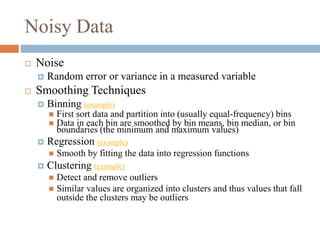
13. Smoothing using Binning Methods
 * Sorted data for price (in dollars): 4, 8, 9, 15, 21, 21, 24,
25, 26, 28, 29, 34
 * Partition into (equi-depth) bins:
 - Bin 1: 4, 8, 9, 15
 - Bin 2: 21, 21, 24, 25
 - Bin 3: 26, 28, 29, 34
 * Smoothing by bin means:
 - Bin 1: 9, 9, 9, 9
 - Bin 2: 23, 23, 23, 23
 - Bin 3: 29, 29, 29, 29
 * Smoothing by bin boundaries: [4,15],[21,25],[26,34]
 - Bin 1: 4, 4, 4, 15
 - Bin 2: 21, 21, 25, 25
 - Bin 3: 26, 26, 26, 34

14. Regression
x
y
y = x + 1
X1
Y1
(salary)
(age)
Example of linear regression

15. Cluster Analysis
cluster
outlier
salary
age

16. 16
Inconsistent Data
 Inconsistent data are handled by:
◦ Manual correction (expensive and tedious)
◦ Use routines designed to detect inconsistencies and manually
correct them. E.g., the routine may use the check global
constraints (age>10) or functional dependencies
◦ Other inconsistencies (e.g., between names of the same attribute)
can be corrected during the data integration process

17. 17
Data Preprocessing
 Why preprocess the data?
 Data cleaning
 Data integration and transformation
 Data reduction
 Discretization and concept hierarchy generation
 Summary

18. Data Integration
 Data integration
◦ combines data from multiple sources into a coherent store
 Schema integration
◦ integrate metadata from different sources
 metadata: data about the data (i.e., data descriptors)
◦ Entity identification problem: identify real world entities from multiple data
sources, e.g., A.cust-id  B.cust-#
 Detecting and resolving data value conflicts
◦ for the same real world entity, attribute values from different sources are
different (e.g., J.D.Smith and Jonh Smith may refer to the same person)
◦ possible reasons: different representations, different scales, e.g., metric vs.
British units (inches vs. cm)

19. Handling Redundant Data in Data
Integration
 Redundant data occur often when integration of multiple
databases
◦ The same attribute may have different names in different databases
◦ One attribute may be a “derived” attribute in another table, e.g., annual
revenue
 Redundant data may be able to be detected by correlation
analysis
 Careful integration of the data from multiple sources may help
reduce/avoid redundancies and inconsistencies and improve
mining speed and quality

20. 20
Pearson’s Product Moment Coefficient of Numerical Attributes A and B
BA
i
N
i=
i
BA
i
N
i
i
σNσ
BA)-Nb(a
σσN
BbAa
BAr
∑
=
∑
= 11=
)-)(-(
,
N: number of records in each attribute
ai, bi (i=1,2,..,N): the ith value of attributes A and B, respectively
σA, σB: the standard deviation of attributes A and B, respectively
BA, : the average values of attributes A and B, respectively
(Eq. 1)

21. 21
Chi-Square Test of Categorical Attributes A and B
A
A1 A2 … Ap
B
B1 A1B1 A2B1 … ApB1
B2 A1B2 A2B2 … ApB2
… … … … …
Bq A1Bq A2Bq … ApBq
Cell (Ai, Bj) represents the joint
event that A= Ai and B= Bj
∑∑
1= 1=
)-(2
2
=1))-1)(-((
p
i
q
j
e
eo
ij
ijij
qpχ : statistic test of the hypothesis
that A and B are independent
2
χ
oij (i=1,2,..,p;j=1,2,…,q): the observed frequency (i.e. actual count) of the joint event (Ai, Bj)
eij (i=1,2,..,p;j=1,2,…,q): the expected frequency of the joint event (Ai, Bj)
N
BBcountAAcount
ij
ji
e
)=(×)=(
=
N: number of records in each attribute
Count(A=Ai): the observed frequency of the event A=Ai
Count(B=Bj): the observed frequency of the event B=Bj
(Eq. 2)
(Eq. 3)

22. Gender Row
Marginmale female
Preferred_
Reading
fiction 250 200 450
non-fiction 50 1000 1050
Column Margin 300 1200 N=1500
90=== 1500
450×300)fiction(×)male(
11 N
countcount
e
210=== 1500
1050×300)fiction-non(×)male(
12 N
countcount
e
360=== 1500
450×1200)fiction(×)female(
21 N
countcount
e
840=== 1500
1050×1200)fiction-non(×)female(
22 N
countcount
e
22

23. 23
Gender Row
Marginmale female
Preferred_
Reading
fiction 250(90) 200(360) 450
non-fiction 50(210) 1000(840) 1050
Column Margin 300 1200 N=1500
840
840)-1000(
360
360)-200(
210
210)-50(
1= 1=
90
90)-250()-(2
22222
+++== ∑∑
p
i
q
j
e
eo
ij
ijij
χ
= 284.44 + 121.90 + 71.11 + 30.48 = 507.93
dof = (2-1)*(2-1)=1
828.10=)1(001.0
2
χ
Conclusion: Gender and Preferred_Reading are strongly correlated!
P< 0.001

24.  Detection and Resolution of Data Value Conflicts
 Attribute values from different sources may be different
 Possible reasons
 Different representations
 e.g. “age” and “birth date”
 Different scaling
 e.g., metric vs. British units
24
Data Integration (Cont.)

25. Data Transformation
 Smoothing: remove noise from data
 Aggregation: summarization, data cube construction
 Generalization: concept hierarchy climbing
 Normalization: scaled to fall within a small, specified range
◦ min-max normalization
◦ z-score normalization
◦ normalization by decimal scaling
 Attribute/feature construction
◦ New attributes constructed from the given ones

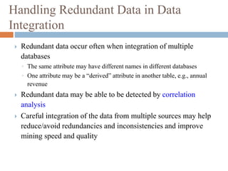
26.  Min-Max Normalization26
Data Normalization
Suppose that the minA and maxA are the minimum and maximum values of an
attribute A. Min-max normalization maps a value, v, of A to v’ in the new range
[new_minA, new_maxA] by computing
AA
A
min-max
min-
='
v
v (new_maxA – new_minA) + new_minA
Suppose the minimum and maximum values for the attribute income are $12,000 and $98,000,
respectively. We would like to map income to the range [0.0, 1.0]. By min-max normalization, a
value of $73,600 for income will be transformed to
716.0=0+)0.0-0.1(12,000-8,0009
12,000-3,6007
(Eq.4 )

27.  Z-Score Normalization
◦ The values of attribute A are normalized based on the mean and
standard deviation of A
27
Data Normalization(Cont.)
A
-
=' σ
Av
v
A value, v, of A is normalized to v’ by computing
:A
σA: the standard deviation of A
Mean of A
Suppose the mean and standard deviation of the values the attribute income are $54,000 and
$16,000, respectively. With z-score normalization, a value of $73,600 for income is transformed
to
225.1=6,0001
54,000-3,6007
(Eq. 5)

28.  Normalization by Decimal Scaling
 Normalize by moving the decimal point of values of attribute A
28
Data Normalization(Cont.)
j
v
v 10
='
A value, v, of A is normalized to v’ by computing
j: the smallest integer such that max(|v’|)<1
Suppose that the recorded values of A range from -986 to 917. The maximum
absolute value of A is 986.
To normalize by decimal scaling, we divide each value by 1,000 (j=3). As a result,
the normalized values of A range from -0.986 to 0.917.
(Eq. 6)

29. Data Preprocessing
 Why preprocess the data?
 Data cleaning
 Data integration and transformation
 Data reduction
 Discretization and concept hierarchy generation
 Summary

30.  Purpose
◦ Obtain a reduced representation of the dataset that is much
smaller in volume, yet closely maintains the integrity of the original
data
 Strategies
◦ Data cube aggregation
 Aggregation operations are applied to construct a data cube
◦ Attribute subset selection
 Irrelevant, weakly relevant, or redundant attributes are detected and
removed
◦ Data compression
 Data encoding or transformations are applied so as to obtain a reduced
or “compressed” representation of the original data
◦ Numerosity reduction
 Data are replaced or estimated by alternative, smaller data
representations (e.g. models)
◦ Discretization and concept hierarchy generation
30
Data Reduction

31.  Purpose
◦ Select a minimum set of attributes (features) such that
the probability distribution of different classes given
the values for those attributes is as close as possible
to the original distribution given the values of all
features
◦ Reduce the number of attributes appearing in the
discovered patterns, helping to make the patterns
easier to understand
 Heuristic Methods
◦ An exhaustive search for the optimal subset of
attributes can be prohibitively expensive .
◦ Stepwise forward selection
◦ Stepwise backward elimination
◦ Combination of forward selection and backward
elimination
◦ Decision-tree induction
31
Attribute/Feature Selection

32.  Stepwise Forward (Example)
◦ Start with an empty reduced set
◦ The best attribute is selected first and added to the
reduced set
◦ At each subsequent step, the best of the remaining
attributes is selected and added to the reduced set
(conditioning on the attributes that are already in the set)
 Stepwise Backward (Example)
◦ Start with the full set of attributes
◦ At each step, the worst of the attributes in the set is
removed
 Combination of Forward and Backward
◦ At each step, the procedure selects the best attribute and
adds it to the set, and removes the worst attribute from the
set
◦ Some attributes were good in initial selections but may not
be good anymore after other attributes have been included
in the set
32
Stepwise Selection

33.  Decision Tree
◦ A mode in the form of a tree structure
◦ Decision nodes
 Each denotes a test on the corresponding attribute which is the
“best” attribute to partition data in terms of class distributions at the
point
 Each branch corresponds to an outcome of the test
◦ Leaf nodes
 Each denotes a class prediction
◦ Can be used for attribute selection
33
Decision Induction

34. 34
Stepwise and Decision Tree Methods for Attribute Selection

35.  Purpose
◦ Apply data encoding or transformations to obtain a
reduced or “compressed” representation of the original
data
 Lossless Compression
◦ The original data can be reconstructed from the
compressed data without any loss of information
◦ e.g. some well-tuned algorithms for string compression
 Lossy Compression
◦ Only an approximation of the original data can be
constructed from the compressed data
◦ e.g. wavelet transforms and principal component
analysis (PCA)
35
Data Compression

36.  Purpose
◦ Reduce data volume by choosing alternative, smaller data
representations
 Parametric Methods
◦ A model is used to fit data, store only the model parameters
not original data (except possible outliers)
◦ e.g. Regression models and Log-linear models
 Non-Parametric Methods
◦ Do not use models to fit data
◦ Histograms
 Use binning to approximate data distributions
 A histogram of attribute A partitions the data distribution of A into
disjoint subsets, or buckets
◦ Clustering
 Use cluster representation of the data to replace the actual data
◦ Sampling
 Represent the original data by a much smaller sample (subset) of
the data
36
Numerosity Reduction

37.  Equal-Width (Example)
◦ The width of each bucket range is the same
 Equal-Frequency (Equal-Depth) (Example)
◦ The number of data samples in each bucket is (about) the same
 V-Optimal (Example)
◦ Bucket boundaries are placed in a way that minimizes the cumulative
weighted variance of the buckets
◦ Weight of a buckle is proportional to the number of samples in the buckle
 MaxDiff (Example)
◦ A MaxDiff histogram of size h is obtained by putting a boundary between
two adjacent attribute values vi and vi+1 of V if the difference between
f(vi+1)·σi+1 and f(vi)·σi is one of the (h − 1) largest such differences (where
σi denotes the spread of vi). The product f(vi)· σi is said the area of v. σi =
vi+1-vi
 V-Optimal and MaxDiff tend to be more accurate and practical than
equal-width and equal-frequency histograms
37
Histogram

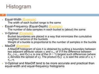
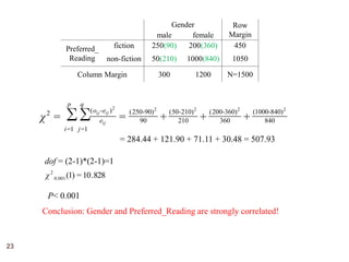
38. 38
Suppose we have the following data:
1, 3, 4, 7, 2, 8, 3, 6, 3, 6, 8, 2, 1, 6, 3, 5, 3, 4, 7, 2, 6, 7, 2, 9
Create a three-bucket histogram
Sorted (24 data samples in total)
1 1 2 2 2 2 3 3 3 3 3 4 4 5 6 6 6 6 7 7 7 8 8 9
Value 1 2 3 4 5 6 7 8 9
Frequenc
y
2 4 5 2 1 4 3 2 1
Bucket Frequency
[1,3] 11
[4,6] 7
[7,9] 6
Histogram
0
2
4
6
8
10
12
[1,3] [4,6] [7,9]
Bucket
Frequency
Equal-Width Histogram

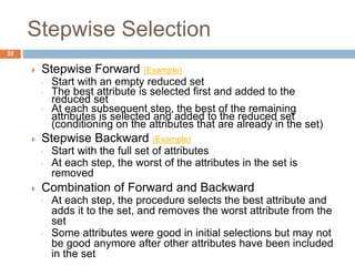
39. 39
Value 1 2 3 4 5 6 7 8 9
Frequenc
y
2 4 5 2 1 4 3 2 1
Bucket Frequency
[1,2] 6
[3,5] 8
[6,9] 10
Equal-Depth Histogram
Histogram
0
2
4
6
8
10
12
[1,2] [3,5] [6,9]
Bucket
Frequency

40. 40
Bucket avg
[1,2] 3
[3,5] 2.67
[6,9] 2.5
V-Optimal Histogram
Value 1 2 3 4 5 6 7 8 9
Frequenc
y
2 4 5 2 1 4 3 2 1
∑
=
2
)-)((
i
i
ub
lbj
iavgjfFor the ith bucket, its weighted variance SSEi =
Suppose the three buckets are [1,2], [3,5], and [6,9]
ubi: the max. value in the ith bucket
lbi: the min. value in the ith bucket
f(j) (j=lbi,…,ubi): the frequency of jth value in the ith bucket
avgi: the average frequency in the ith bucket
2=3)-4(+)3-2(= 22
1SSE
67.8=2.67)-1(+2.67)-2(+).672-5(= 222
2SSE
5=2.5)-1(+2.5)-2(+2.5)-3(+).52-4(= 2222
3SSE
Accumulated weight variance SSE ∑=
i
iSSE
67.15=5+67.8+2=SSE

41. 41
Value 1 2 3 4 5 6 7 8 9
Frequen
cy
2 4 5 2 1 4 3 2 1
Bucket Frequency
[1,3] 11
[4,5] 3
[6,9] 10
MaxDiff Histogram
Histogram
0
2
4
6
8
10
12
[1,3] [4,5] [6,9]
Bucket
Frequency

42.  Simple Random Sampling without Replacement
(SRSWOR)
◦ Draw s of the N records from dataset D (s<N), with no record
can be drawn more than once
 Simple Random Sampling with Replacement (SRSWR)
◦ Each time a record is drawn from D, it is recorded and then
placed back to D, so it may be drawn more than once
 Cluster Sampling
◦ Records in D are first divided into groups or clusters, and a
random sample of these clusters is then selected (all records
in the selected clusters are included in the sample)
 Stratified Sampling
◦ Records in D are divided into subgroups (or strata), and
random sampling techniques are then used to select sample
members from each stratum
42
Sampling

43. 43
Raw Data
Stratified Sampling Cluster Sampling

44.  Discretization
◦ Reduce the number of values for a given continuous attribute
by dividing the range of the attribute into intervals
◦ Interval labels can then be used to replace actual data values
◦ Supervised versus unsupervised
 Supervised discretization process uses class information
 Unsupervised discretization process does not use class information
◦ Techniques
 Binning (unsupervised)
 Histogram (unsupervised)
 Clustering (unsupervised)
 Entropy-based discretization (supervised)
 Concept Hierarchies
◦ Reduce the data by collecting and replacing low level
concepts by higher level concepts
44
Discretization and Concept
Hierarchy

45. 45
Concept Hierarchy for Attribute Price

46.  Entropy (“Self-Information”)
◦ A measure of the uncertainty associated with a random
variable in information theory
46
Entropy-Based Discretization
Given m classes, c1, c2, …, cm, in dataset D, the entropy
of D is
∑
1=
2 )(log-=
m
i
ii ppH(D)
pi: the probability of class ci in D, calculated as:
pi= (# of records of ci) /
|D|
|D|: # of records in D

47. 47
A dataset has 64 records, among which 16 records
belong to c1 and 48 records belong to c2
p(c1) = 16/64 =0.25
p(c2) = 48/64 = 0.75
H(D) = -[0.25·log2(0.25) + 0.75·log2(0.75)] = 0.811

48.  Given a dataset D, if D is discretized into two intervals
D1 and D2 using boundary T, the entropy after
partitioning is
48
Entropy-Based Discretization
(Cont.)
)(+)(=),( 2||
||D
1||
||D 21
DHDHTDH DD
 The boundary that minimizes the entropy function over all
possible boundaries is selected as a binary discretization.
 The process is recursively applied to partitions obtained until
some stopping criterion is met
 e.g.H(D) – H(D,T) < δ
|D1|, |D2|: # of records in D1 and D2, respectively
H(D1), H(D2): entropy of D1 and D2, respectively

49. 49
A dataset D has 64 records, among which 16 records belong to c1 and 48
records belong to c2
(1) D is divided into two intervals: D1 has 45 records (2 belonging to c1 and 43
belonging to c2) and D2 has 19 records (14 belonging to c1 and 5 belonging
to c2)
(2) D is divided into two intervals: D3 has 40 records (10 belonging to c1 and 30
belonging to c2) and D4 has 24 records (6 belonging to c1 and 18 belonging
to c2)(1)
H(D1) = -[2/45*log2(2/45)+43/45*log2(43/45)] =
0.2623
H(D2) = -[14/19*log2(14/19)+5/19*log2(5/19)] =
0.8315
H(D,T1) = (45/64)*0.2623+(19/64)*0.8315 = 0.4313
(2)
H(D3) = -[10/40*log2(10/40)+30/40*log2(30/40)] =
0.8113
H(D4) = -[6/24*log2(6/24)+18/24*log2(18/24)] =
0.8113
H(D,T2) = (40/64)*0.8113+(24/64)*0.8113 = 0.8113
H(D,T1) < H(D,T2), so T1 is better than T2