Interconnections of hybrid systems

Interconnections of hybrid systems
Michael Kosmykov
3. February 2012, Fachhochschule Erfurt

Centre for
Industrial Mathematics
Outline
1 Motivation
2 Hybrid system
3 Extension of hybrid time domain
4 Conclusion and outlook
2 / 40Motivation Hybrid system Hybrid domain Summary

Centre for
Logistics network as hybrid system from PhD thesis:
3 production sites (D, F, E) for
Liquidring-Vaccum (LRVP), Industrial (IND)
and Side-channel (SC) pumps
5 distribution centers (D, NL, B, F, E)
33 ﬁrst and second-tier suppliers for the
production of pumps
90 suppliers for components that are needed
for the assembly of pump sets
More than 1000 customers

Centre for
Logistics network as hybrid system from PhD thesis:
Instability leads to:
High inventory costs
Large number of unsatisﬁed orders
Loss of customers

Centre for
Analysis steps:
1 Mathematical modelling
2 Model reduction, if the model size is large
3 Stability analysis

Centre for
Modelling approaches
Discrete system:
Decentralized supply chain
Re-entrant/queueing
system
”Bucket brigade”
Continuous system:
Ordinary differential equations
- Damped oscillator model
Multilevel network
Partial differential equations
Hybrid model:
Hybrid system
Switched system
Stochastic system:
Stochastic system
Queueing/fluid network

Centre for
Hybrid system
xi - state of logistics location Σi (stock level)
u - external input (customer orders, raw material)
State xi changes continuously during production.
Σi
t0
xi (0)
xi (t)
xi

Centre for
Hybrid system
When a truck picks up ﬁnished material, state xi ”jumps”.
Σi
t0
xi (0)
xi (t)
t1
xi

Centre for
Hybrid system
After the jump state xi changes again continuously.
Σi
t0
xi (0)
xi (t)
t1
xi

Centre for
Hybrid system
Hybrid dynamics of location Σi :
˙xi = fi (x1, . . . , xn, u), (x1, . . . , xn, u)∈Ci production
x+
i = gi (x1, . . . , xn, u), (x1, . . . , xn, u)∈Di transportation
Σi
t0
xi (0)
xi (t)
t1 t2 t3
xi

Centre for
Hybrid system
The whole network Σ is given by interconnection of individual
locations:
Hybrid dynamics of the whole logistics network Σ:
˙x = ?, (x1, . . . , xn, u) ∈ C =? overall production
x+ = ?, (x1, . . . , xn, u) ∈ D =? overall transportation

Centre for
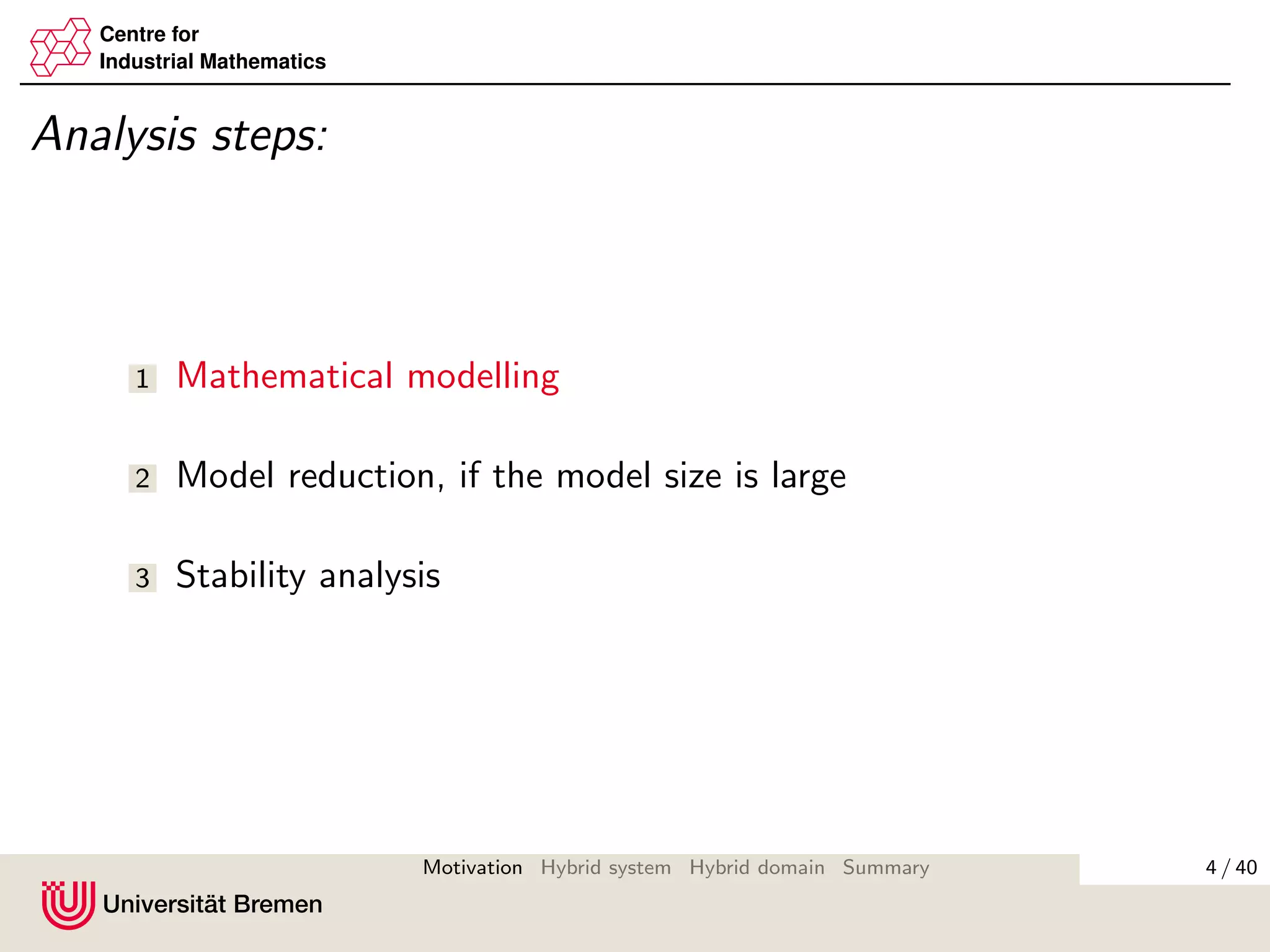
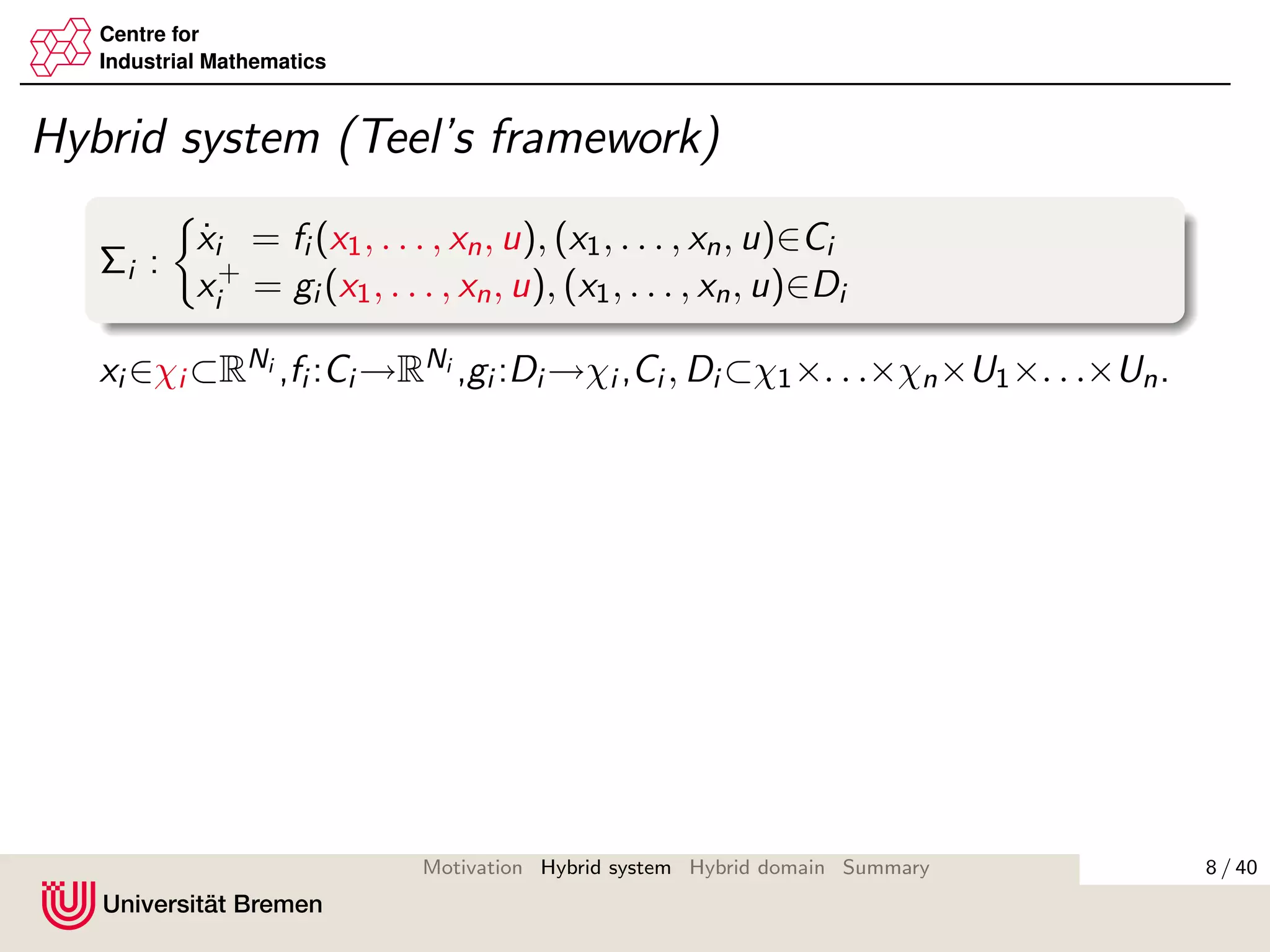
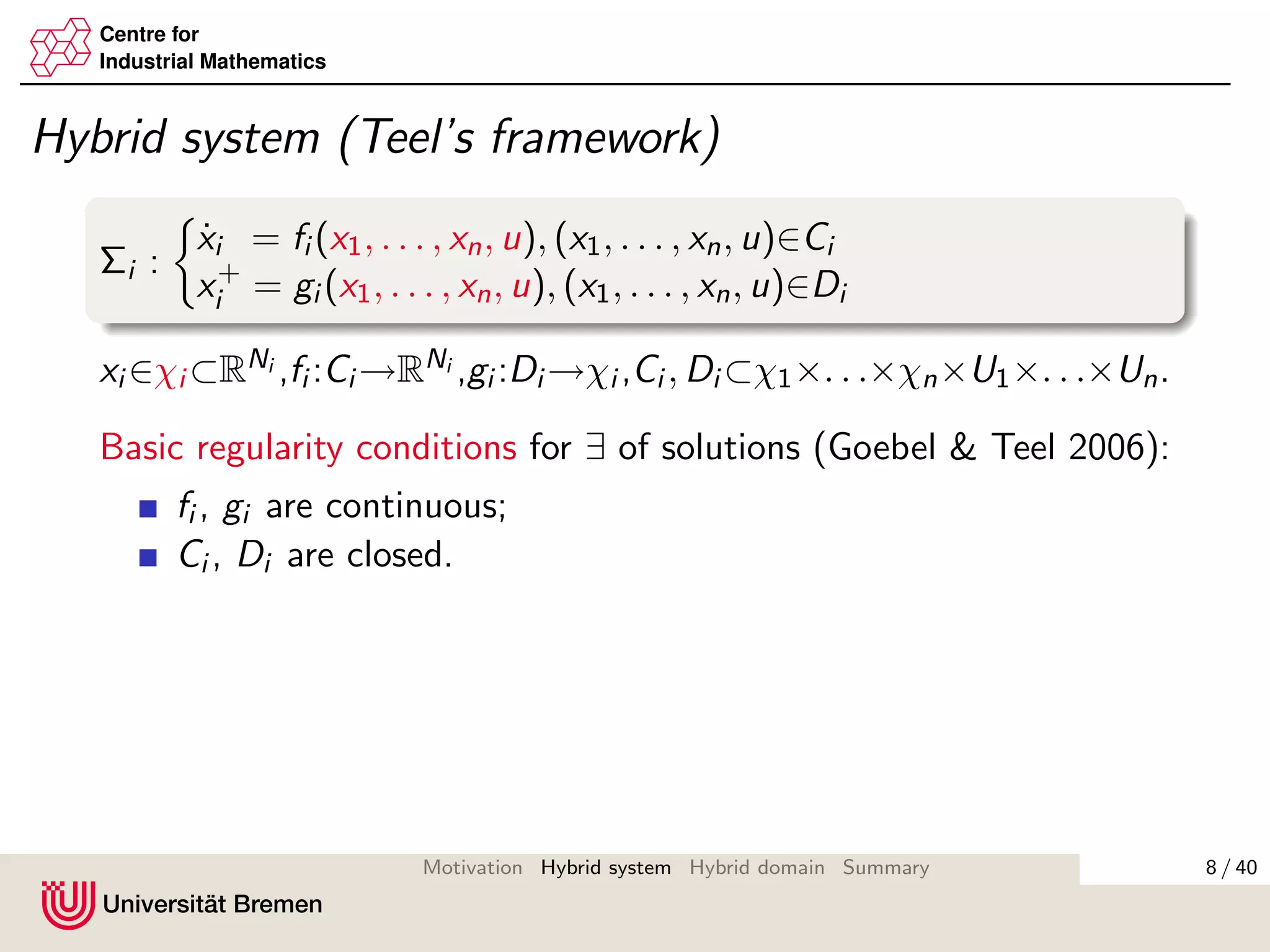
Hybrid system (Teel’s framework)
Σi :
˙xi = fi (x1, . . . , xn, u), (x1, . . . , xn, u)∈Ci
x+
i = gi (x1, . . . , xn, u), (x1, . . . , xn, u)∈Di
xi ∈χi ⊂RNi ,fi :Ci →RNi ,gi :Di →χi ,Ci , Di ⊂χ1×. . .×χn×U1×. . .×Un.

Centre for
Σi :
˙xi = fi (x1, . . . , xn, u), (x1, . . . , xn, u)∈Ci
x+
i = gi (x1, . . . , xn, u), (x1, . . . , xn, u)∈Di
Basic regularity conditions for ∃ of solutions (Goebel & Teel 2006):
fi , gi are continuous;
Ci , Di are closed.

Centre for
Σi :
˙xi = fi (x1, . . . , xn, u), (x1, . . . , xn, u)∈Ci
x+
i = gi (x1, . . . , xn, u), (x1, . . . , xn, u)∈Di
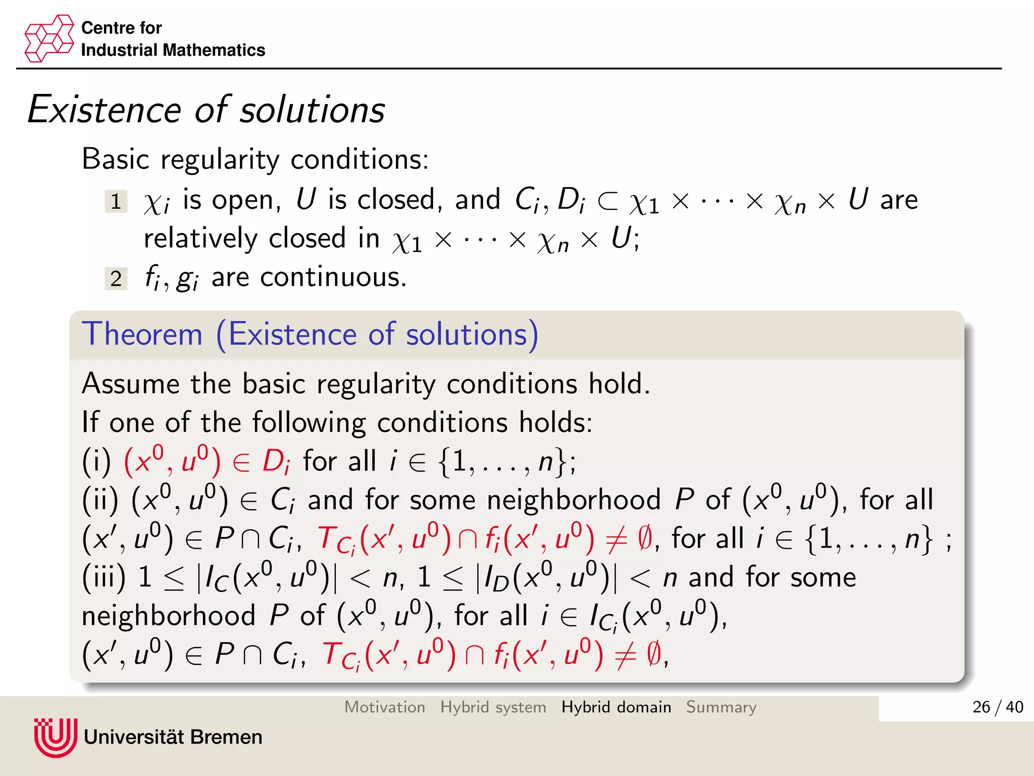
Basic regularity conditions for ∃ of solutions (Goebel & Teel 2006):
fi , gi are continuous;
Ci , Di are closed.
Solution xi (t, k) is deﬁned on hybrid time domain:
dom xi := ∪[tk, tk+1]×{k}
t is time and k is number of the last jump.

Centre for
Stability notions
Global stability (GS)
Hybrid system is called globally stable (GS), if there exists σ ∈ K∞
such that any solution x satisﬁes
|x(t, k)| ≤ σ(|x0|), ∀(t, k) ∈ dom x.
Global attractivity (GA)
Hybrid system is called globally attractive (GA), if for each > 0
and r > 0 there exists T > 0 such that, for any solution x,
|x(0, 0)| ≤ r, (t, k) ∈ dom, x, and t + k ≥ T imply |x(t, k)| ≤ .
Global asymptotical stability (GAS)
Hybrid system is called globally asymptotically stable (GAS), if it is
both GS and GA.

Centre for
Example: Bouncing ball
˙x=
x2
−γ
=:f (x), x∈C,
x+=
x1
−λx2
=:g(x), x∈D.
x1 - height
x2 - velocity
C := {(x, u) ∈ R2 × U : x1 ≥ 0},
D := {(x, u) ∈ R2 × U : x1 =
0, x2 ≤ 0},
γ - gravitation force,
λ ∈ (0, 1) - restitution coeﬃcient

Centre for
Example: Bouncing ball
Figure: Trajectory of the
bouncing ball.
Figure: Time domain of the
bouncing ball.

Centre for
Zeno solutions
Definition (Ames et. al. 2006)
The solution (x, u) possesses:
chattering Zeno behaviour, if there exists a finite K ≥ 0 such
that (t, k), (t, k + 1) ∈ dom x for all k ≥ K;
genuinely Zeno behaviour, if there exists a finite T ≥ 0 such
that for all (s, k), (t, k + 1) ∈ dom x, s < t < T.
Bouncing ball possesses the genuinely Zeno behaviour with
T = tmax = 2h
γ + 2λ
1−λ
2h
γ .
Furthermore, it is GAS (Sanfelice and Teel 2008).

Centre for
Interconnection of hybrid systems
Σ:
˙x = f (x, u), (x, u)∈C
x+ = g(x, u), (x, u)∈D
χ:=χ1×. . .×χn, x:=(xT
1 , . . ., xT
n )T ∈χ⊂RN, N:= Ni , C:= ∩ Ci ,
D:= ∪ Di , f :=(f T
1 , . . ., f T
n )T , g:=(gT
1 , . . ., gT
n )T with
gi (x, u) :=
gi (x, ui ), if (x, u) ∈ Di ,
xi , otherwise .

Centre for
Example of interconnection of hybrid systems
two bouncing balls with states x1 ∈ R2 and x2 ∈ R2
respectively.
they are interconnected by an elastic elastic coeﬃcient k ≥ 0
horizontal distance between the balls is neglected
the balls do not hit each other.
The interaction force due to the elastic spring is given by
±k(x1
1 − x2
1 ).

Centre for
Their dynamics is given by:
First ball
˙x1
=
x1
2
−γ − k(x1
1 − x2
1 )
, (x1
, x2
) ∈ C1
={(x1
, x2
) ∈ R4
: x1
1 ≥ 0},
x1+
=
x1
1
−λx1
2
, (x1
, x2
) ∈ D1
={(x1
, x2
) ∈ R4
: x1
1 = 0, x1
2 ≤ 0},
Second ball
˙x2
=
x2
2
−γ + k(x1
1 − x2
1 )
, (x1
, x2
) ∈ C2
={(x1
, x2
) ∈ R4
: x2
1 ≥ 0},
x2+
=
x2
1
−λx2
2
, (x1
, x2
) ∈ D2
={(x1
, x2
) ∈ R4
: x2
1 = 0, x2
2 ≤ 0},

Centre for
Dynamics of interconnection
˙z = f (z), z ∈ C := C1 ∩ C2,
z+ = g(z), z ∈ D := D1 ∪ D2 ∈ R4,
where z := (x1T
, x2T
)T , f (z) := (f 1T , f 2T )T ,
g(z) := (g1T , g2T )T ,
gi
(z) = gi
(x1
, x2
) :=
gi (x1, x2), if (x1, x2) ∈ Di ,
xi , otherwise .

Centre for
Drawback
Taking x1
1 (0) = x1
2 (0) = 0 and x2
1 (0) = h > 0, x2
2 (0) = v ∈ R the
hybrid arc
x1
1 (t, j) = x1
2 (t, j) = 0, x2
1 (t, j) = h, x2
2 (t, j) = v
is a solution with hybrid time domain {(0, j)}∞
j=0.
Thus tmax = 0 and the system jumps inﬁnitely many times from a
non-zero state to the same state ⇒ the solution possesses
chattering Zeno solution ⇒ No physical meaning! and furthermore
is no more GAS.

Centre for
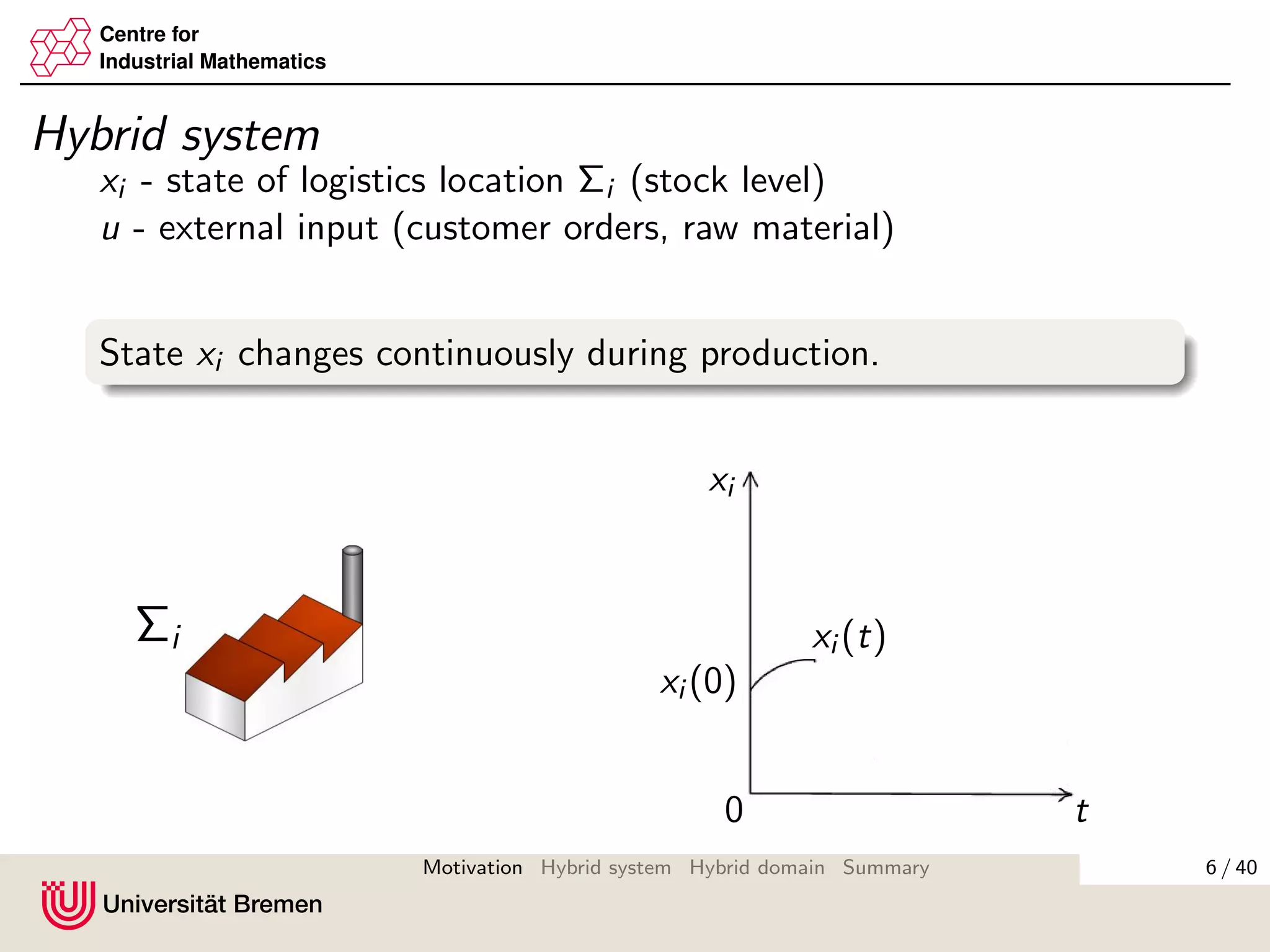
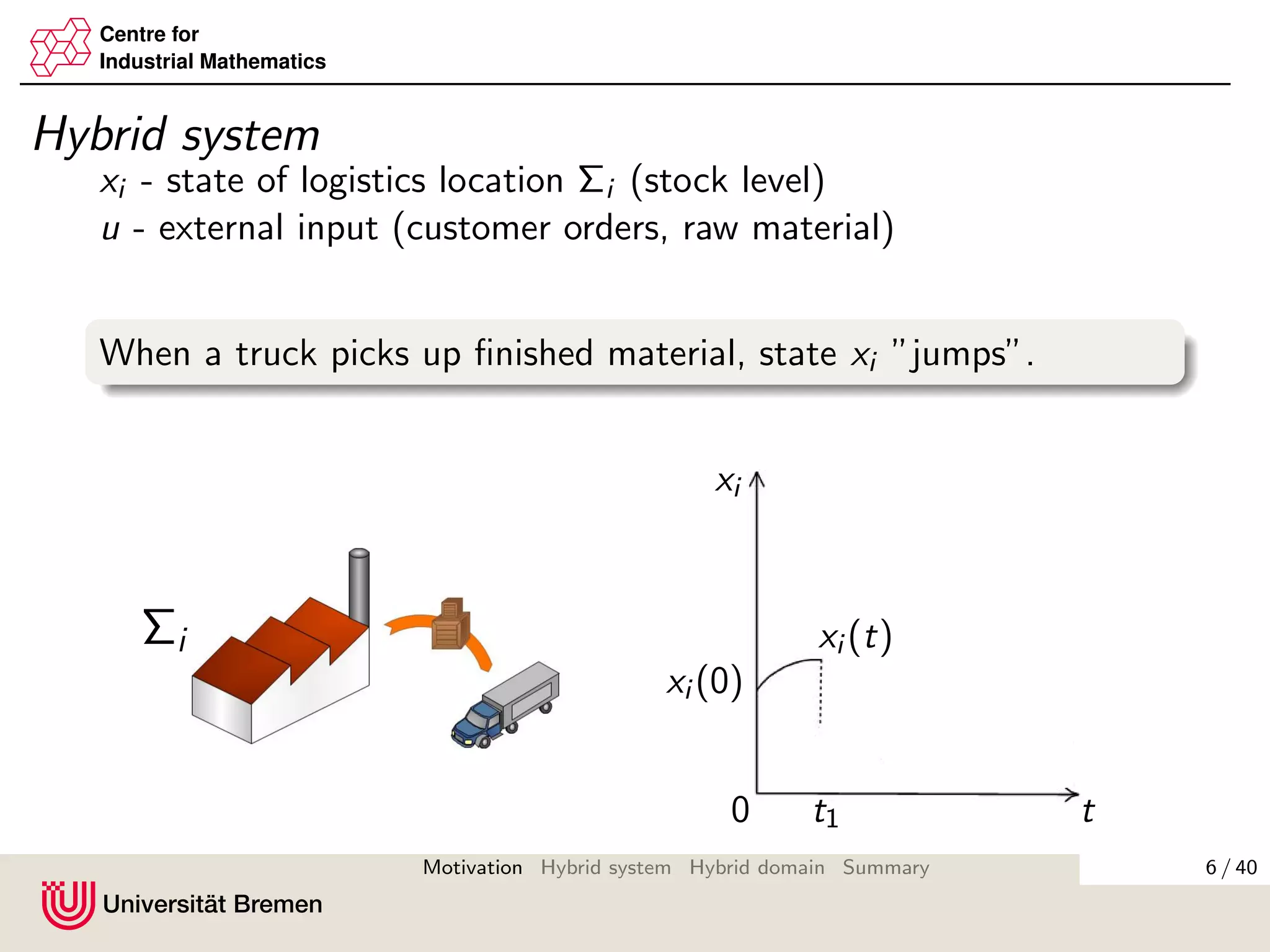
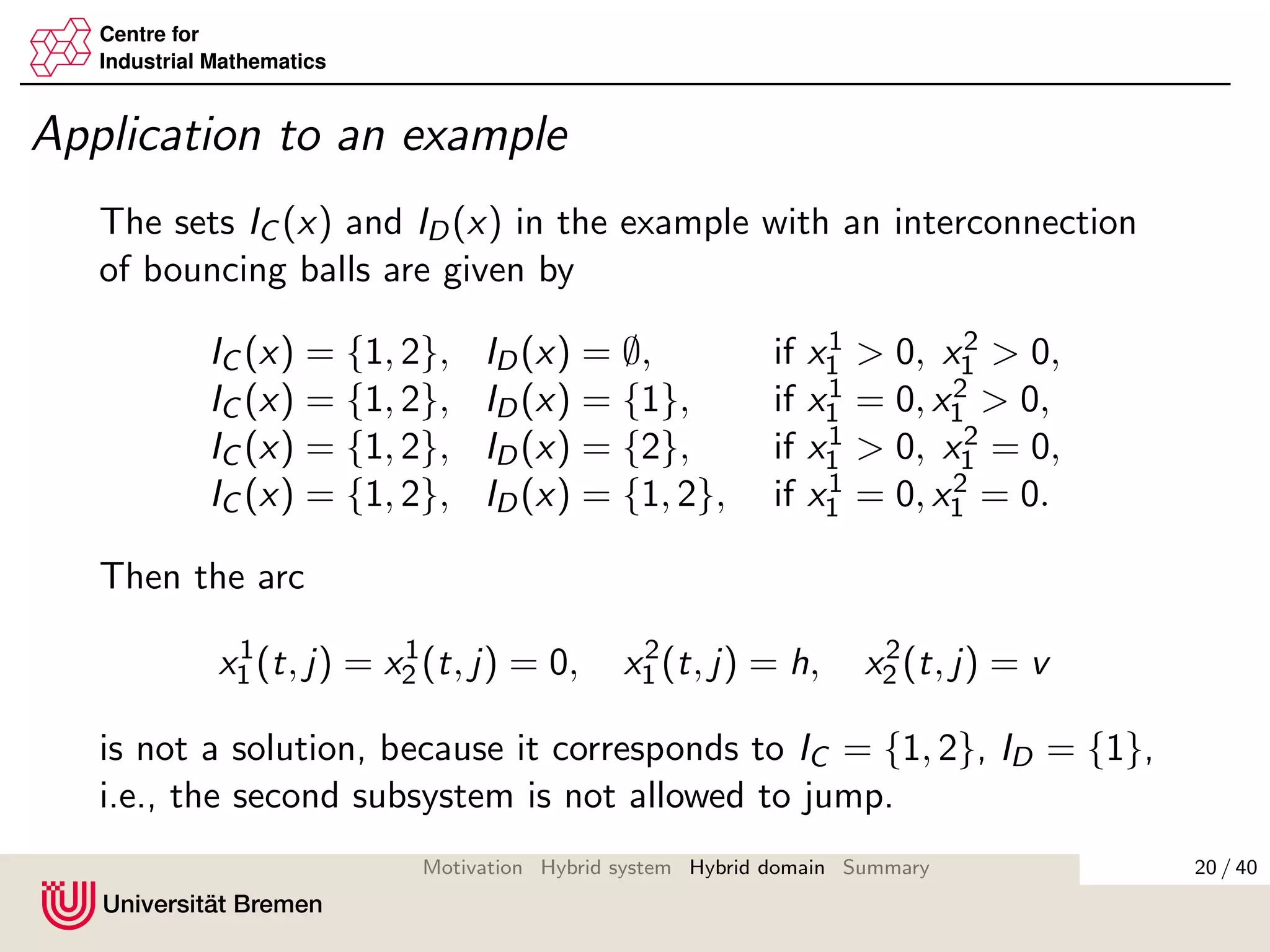
Our approach
We take into account which of the system can jump by:
IC (x, u):={i : (x, u) ∈ Ci }, ID(x, u):={i : (x, u) ∈ Di }.
Then dynamics is given by
˙xi = fi (x, u), i ∈ IC (x, u),
x+
i = gi (x, u), i ∈ ID(x, u).
Hybrid time domain considers the jumps of the subsystems
separately:
domk1,...,kn := ∪[tk, tk+1] × {k1, . . . , kn} ⊂ R+ × Nn
+,
where k = k1 + · · · + kn and ki ∈ N+ calculates the jumps of
the ith subsystem.
ti
max

Centre for
Solution
(i) (x(0, 0), u(0, 0)) ∈ Ci ∪ Di , ∀i
(ii) for i ∈ IC (x1
1 (t, k), . . . , xn(t, k), u(t, k)),
˙xi (t, k)=fi (x1
1 (min{t, t1
max}, k), . . ., xn(min{t, tn
max}, k), u(t, k))
(iii) for all (t, k) ∈ domk x with (t, k + p) ∈ domk x p ≥ 1
for i ∈ ID(x1
1 (t, k), . . . , xn(t, k), u(t, k),
x+
i (min{t, tk
max}, k+p) =
gi (x1
1 (min{t, t1
max}, k), . . . , xn(min{t, tn
max}, k), u(t, k))
k = (k1, . . . , kn) ∈ Nn
+

Centre for
Application to an example
The sets IC (x) and ID(x) in the example with an interconnection
of bouncing balls are given by
IC (x) = {1, 2}, ID(x) = ∅, if x1
1 > 0, x2
1 > 0,
IC (x) = {1, 2}, ID(x) = {1}, if x1
1 = 0, x2
1 > 0,
IC (x) = {1, 2}, ID(x) = {2}, if x1
1 > 0, x2
1 = 0,
IC (x) = {1, 2}, ID(x) = {1, 2}, if x1
1 = 0, x2
1 = 0.
Then the arc
x1
1 (t, j) = x1
2 (t, j) = 0, x2
1 (t, j) = h, x2
2 (t, j) = v
is not a solution, because it corresponds to IC = {1, 2}, ID = {1},
i.e., the second subsystem is not allowed to jump.

Centre for
GAS
Adaptation of Matrosov’s theorem
Let a hybrid system be GS. Then, it is GAS if ∃m∈N, and for each
0 < δ < ∆,
a number µ > 0,
continuous wc,j : (∪i
¯Ci ) ∩ ΩIC (x)(δ, ∆) → R,
wd,j : (∪i
¯Di ) ∩ ΩID (x)(δ, ∆) → R, j ∈ {1, . . . , m},
Vj : RN 0 → R, j ∈ {1, . . . , m} are C1 on an open set
containing (∪i
¯Ci ) ∩ ΩIC (x)(δ, ∆),

Centre for
GAS
Adaptation of Matrosov’s theorem (continued)
such that, for each j ∈ {1, . . . , m}
i) |Vj (x)| ≤ µ ∀x ∈ (∪i
¯Ci )∪(∪i Di ) ∪ (∪i gi (Di ))∩Ω(δ, ∆)
ii) Vj (x)IC
, (f T
1 , . . ., f T
n )T
IC
≤wc,j (x), ∀x∈(∪i Ci )∩ΩIC (x)(δ, ∆)
iii)Vj ((gT
1 , . . . , gT
n )T
(˜x))−Vj (˜x)≤wd,j (x), ∀x∈(∪i Di )∩ΩID (x)(δ, ∆)
and with wc,0, wd,0 : RN → {0} and wc,m+1, wd,m+1 : RN → {1}
such that for each l ∈ {0, . . . , m},
1) if x ∈ (∪i
¯Ci ) ∩ Ω(δ, ∆) and wc,j (x) = 0 for all j ∈ {0, . . . , l}
then wc,l+1(x) ≤ 0,
2) if x ∈ (∪i
¯Di ) ∩ Ω(δ, ∆)ID (x) and wd,j (x) = 0 for all
j ∈ {0, . . . , l} then wd,l+1(x) ≤ 0.

Centre for
Application of Matrosov’s theorem to an interconnection
of bouncing balls
System is GS (Sanfelice and Teel 2008).
Deﬁne z := (x1, x2)T and
V1(z) := V1(x1, x2) := 1
2(x1
2
2
+ x2
2
2
) + γx1
1 + γx2
1 + k
2 (x2
1 − x1
1 )2
V2(z) := V2(x1, x2) = γx1
2 + γx2
2 .
Consider the following four cases:
both components of the state ﬂow continuously:
˙V1(z) = x1
2 (−kx1
1 + kx2
1 − γ) + x2
2 (kx1
1 − kx2
1 − γ) + γx1
2 +
γx2
2 + k(x2
1 − x1
1 )(x2
2 − x1
2 ) = 0,
˙V2(z) = −2γ2

Centre for
Application of Matrosov’s theorem to an interconnection
of bouncing balls
both components of the state jump:
V1(z+) − V1(z) = −1
2(1 − λ2)x1
2
2
− 1
2(1 − λ2)x2
2
2
,
V2(z+) − V2(z) = −(1 + λ)γ(x1
2 + x2
2 )
the first component of the state jumps and the second flows
continuously:
V1(z+) − V1(z) = −1
2(1 − λ2)x1
2
2
,
V2(z+) − V2(z) = −(1 + λ)γx1
2
the first component of the state flows continuously and the
second jumps:
V1(z+) − V1(z) = −1
2(1 − λ2)x2
2
2
,
V2(z+) − V2(z) = −(1 + λ)γx2
2
Then the interconnected system is GAS.

Centre for
Trajectories
Figure: Trajectories two bouncing
balls connected by a spring.
Figure: Time domain of two
interconnected balls.

Centre for
Existence of solutions
Basic regularity conditions:
1 χi is open, U is closed, and Ci , Di ⊂ χ1 × · · · × χn × U are
relatively closed in χ1 × · · · × χn × U;
2 fi , gi are continuous.
Theorem (Existence of solutions)
Assume the basic regularity conditions hold.
If one of the following conditions holds:
(i) (x0, u0) ∈ Di for all i ∈ {1, . . . , n};
(ii) (x0, u0) ∈ Ci and for some neighborhood P of (x0, u0), for all
(x , u0) ∈ P ∩ Ci , TCi
(x , u0) ∩ fi (x , u0) = ∅, for all i ∈ {1, . . . , n} ;
(iii) 1 ≤ |IC (x0, u0)| < n, 1 ≤ |ID(x0, u0)| < n and for some
neighborhood P of (x0, u0), for all i ∈ ICi
(x0, u0),
(x , u0) ∈ P ∩ Ci , TCi
(x , u0) ∩ fi (x , u0) = ∅,

Centre for
Theorem (Existence of solutions, continued)
then there exists a solution pair (x, u) for hybrid system with
(t, ¯k) ∈ domx for some t > 0 or ¯k ≡ (0, . . . , 0)T ∈ Nn
+.
Furthermore, if for all i ∈ {1, . . . , n}, gi (Di ) ∈ Ci ∪ Di , then there
exists a solution with t > 0, ¯k ∈ Nn
+ such that
(x(t, ¯k), u(t, ¯k)) ∈ Ci ∪ Di .
Proof
We consider all the cases separately and construct solutions for
them explicitly.

Centre for
Another problem (semi-genuinely Zeno solution)
Example:
two balls with masses m1 and m2 such that m2 > m1.
the ﬁrst ball was launched at an angle 0 < θ < π
2 to the
horizontal line and then bounces with initial velocity v1
towards the second ball
the second balls rolls with constant velocity v2 towards the
ﬁrst ball.

Centre for
Dynamics in C
For
(x1, y1, v1, x2, y2, v2, q)∈C={(x1, y1, v1, x2, y2, v2, q)∈R7 : y1 ≥ 0}:



˙x1 =
v1 cos θ, if q = 0,
−v1, if q = 1
˙y1 =
v1 sin θ − gt, if q = 0,
0, if q = 1
˙v1 = 0



˙x2 =
−v2, if q = 0,
v2, if q = 1
˙y2 = 0
˙v2 = 0
˙q = 0
q - logical variable that determines, whether they have already
collided.

Centre for
Dynamics in D = D1 ∪ D2
At the bounce in
(x1, y1, v1, x2, y2, v2, q)∈D1={(x1, y1, v1, x2, y2, v2, q)∈R7 : y1 =
0, v1 ≥ 0, q = 0}: 


x+
1 = x1
y+
1 = y1
v+
1 = µv1



x+
2 = x1
y+
2 = y1
v+
2 = v2
q+
= q

Centre for
Dynamics in D = D1 ∪ D2
At the collision in (x1, y1, v1, x2, y2, v2, q) ∈ D2 =
{(x1, y1, v1, x2, y2, v2, q) ∈ R7 : x1 = x2, v1 ≥ 0, q = 0}:



x+
1 = x1
y+
1 = y1
v+
1 = v1 = 2m2
m1+m2
v2



x+
2 = x1
y+
2 = y1
v+
2 = v2 = m2−m1
m1+m2
v2
q+
= 1

Centre for
Trajectories
Figure: Trajectories before the stop of the ﬁrst ball.
The ﬁrst ball ”stops” earlier due to the loss of energy, i.e. at
t1
max < t2
max

Centre for
Trajectories
Figure: Trajectories before the collision.
After some time the second ball reaches the ﬁrst, i.e. at
(x1, y1, v1, x2, y2, v2, q) ∈ D2 and they collide.

Centre for
Trajectories
Figure: Trajectories after the collision.
As m2 > m1, the ﬁrst ball begins to move again in opposite
direction to the second ball.
Thus hybrid time domain of the ﬁrst ball is extended beyond t1
max!

Centre for
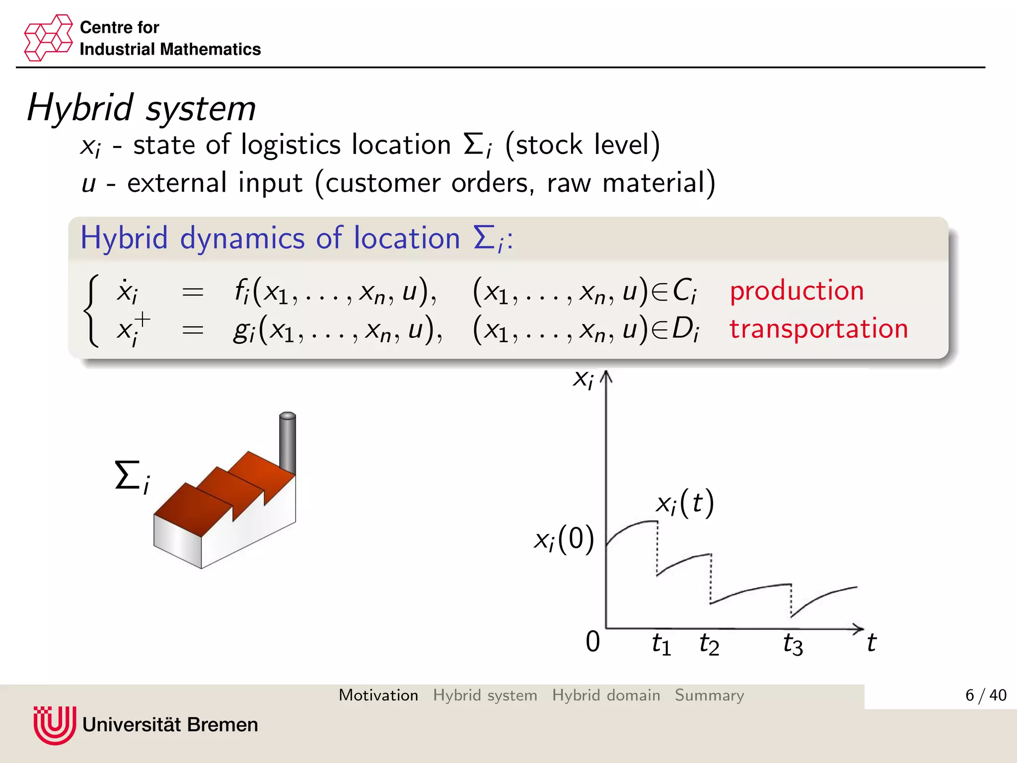
Possible solution
Instead of considering min{t, ti
max}, we consider intervals
[ti,ki
min, ti,ki
max], ki = 0, 1, 2, . . .
where system i is ”active”, and intervals
[ti,ki
max, ti,ki +1
min ],
where system i is ”passive” (in physical sense).
θi (t) :=
t, ti,ki
min < t < ti,ki
max
ti,ki
max, ti,ki
max < t < ti,ki +1
min
identiﬁes, whether at time t the system i is ”active” or ”passive”.

Centre for
Deﬁnition of solution
Hybrid arc x and hybrid input u are a solution pair, if
(i) (x(0, 0), u(0, 0)) ∈ Ci ∪ Di , ∀i
(ii) for i ∈ IC (x1
1 (t, k), . . . , xn(t, k), u(t, k)),
˙xi (t, k) = fi (x1
1 (θ1(t), k), . . . , xn(θn(t), k), u(t, k));
(iii) for all (t, k) ∈ domk x with (t, k + p) ∈ domk x where p ≥ 1
for i ∈ ID(x1
1 (t, k), . . . , xn(t, k), u(t, k),
x+
i (θi (t), k + p) = gi (x1
1 (θ1(t), k), . . . , xn(θn(t), k), u(t, k)).
k := (k1, . . . , kn) ∈ Nn
+

Centre for
Application to an example
1 The second ball is always ”active” ⇒ k2 = 0, t2,k2
min = 0,
t2,k2
max = ∞.
2 The first ball first bounces from t1,0
min = 0 till t1,0
max.
3 Then it lies on the floor.
4 At t1,1
min the two balls collide
5 And the first ball flows till t1,1
max = ∞ ⇒ Thus k1 = 1.

Centre for
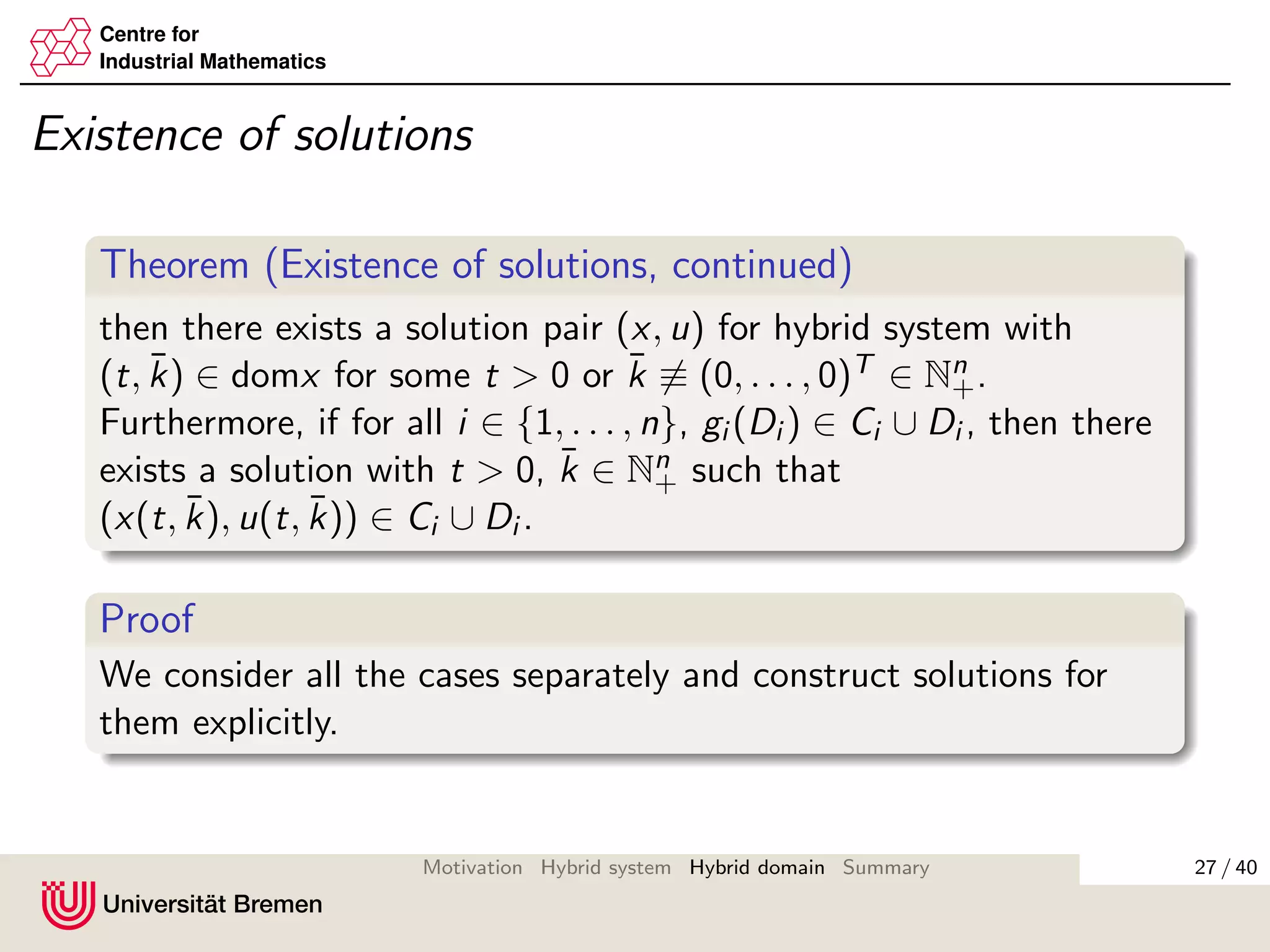
Theorem (Existence of solutions, continued)
then there exists a solution pair (x, u) for hybrid system with
(t, ¯k) ∈ domx for some t > 0 or ¯k ≡ (0, . . . , 0)T ∈ Nn
+.
Furthermore, if for all i ∈ {1, . . . , n}, gi (Di ) ∈ Ci ∪ Di , then there
exists a solution with t > 0, ¯k ∈ Nn
+ such that
(x(t, ¯k), u(t, ¯k)) ∈ Ci ∪ Di .
Proof
For each interval [ti,ki
min, ti,ki +1
min ] we consider all the cases separately
and construct solutions for them explicitly. Then we concatenate
the solutions on the intervals.

Centre for
Conclusion
Hybrid systems allow to describe complex dynamics like
behaviour of logistics networks
Hybrid systems may possess solutions with no physical
meaning (Zeno behaviour) ⇒ hybrid systems have to be used
very carefully
If subsystems in interconnections of hybrid systems possess
Zeno behaviour, one can extend the notion of time domain to
exclude such solutions

Centre for
Thank you for your attention!

Interconnections of hybrid systems

More Related Content

What's hot

Viewers also liked

Similar to Interconnections of hybrid systems

Recently uploaded

Interconnections of hybrid systems