Download as PDF, PPTX
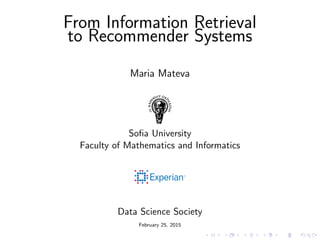


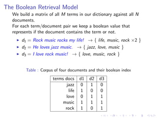
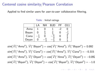
![The Inverted Index and the Vector-Space Model
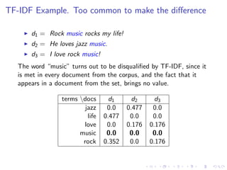
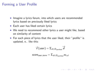
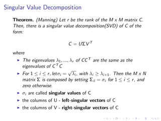
Term-document matrix C[MxN]for M terms and N documents.
Table : We need weights for each term-document couple
terms docs d1 d2 ... dN
t1 w1,1 w1,2 ... w1,N
t2 w2,1 w2,2 ... w2,N
... ... ... ... ...
tM wM,1 wM,2 ... wM,N](https://image.slidesharecdn.com/informationretrievaltorecommendersystems-150519143029-lva1-app6891/85/Information-retrieval-to-recommender-systems-13-320.jpg)


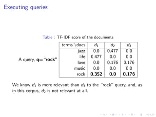


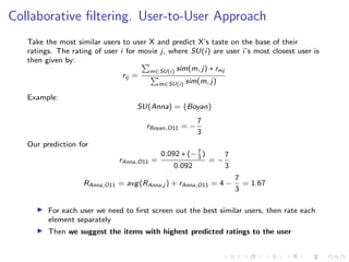


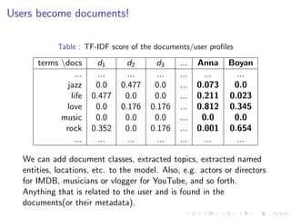
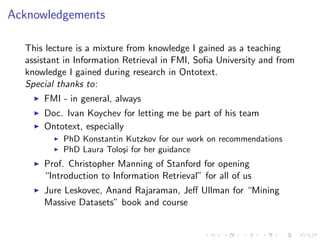
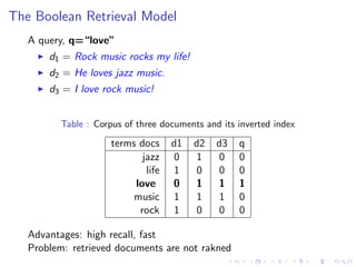
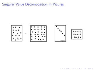
![The problem with dimensionality and sparsity
Imagine...
N = 10,000,000 users
200, 000 items
in a vector-space of M = 1,000,000 terms
how do we use our sparse matrix C[NxM]?](https://image.slidesharecdn.com/informationretrievaltorecommendersystems-150519143029-lva1-app6891/85/Information-retrieval-to-recommender-systems-41-320.jpg)
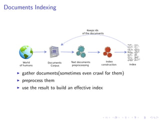
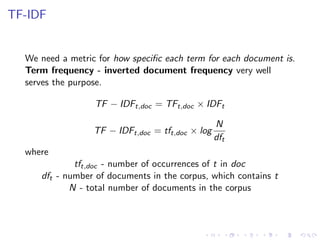
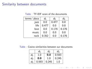
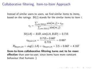
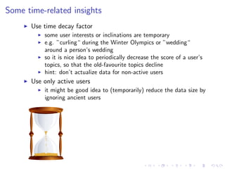
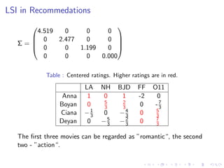
![The problem with dimensionality and sparsity
Imagine...
N = 10,000,000 users
200, 000 items
in a vector-space of M = 1,000,000 terms
how do we use our sparse matrix C[NxM]?
OMG!!! This is big data!!!
;)](https://image.slidesharecdn.com/informationretrievaltorecommendersystems-150519143029-lva1-app6891/85/Information-retrieval-to-recommender-systems-42-320.jpg)


This document provides an introduction to information retrieval and recommender systems. It begins with defining information retrieval as finding documents that satisfy an information need from large collections. It then discusses how documents are indexed and preprocessed, including tokenization, stopwords removal, and lemmatization. Boolean and vector space retrieval models are introduced. The document also defines recommender systems as systems that suggest items of interest to users based on their preferences. It describes collaborative filtering and content-based recommender approaches.


![[系列活動] 人工智慧與機器學習在推薦系統上的應用](https://cdn.slidesharecdn.com/ss_thumbnails/merged-161217165734-thumbnail.jpg?width=640&height=640&fit=bounds)


![[Data Meetup] Data Science in Finance - Building a Quant ML pipeline](https://cdn.slidesharecdn.com/ss_thumbnails/buildingaquantmlpipeline-191009091209-thumbnail.jpg?width=640&height=640&fit=bounds)


![[Data Meetup] Data Science in Finance - Factor Models in Finance](https://cdn.slidesharecdn.com/ss_thumbnails/factormodelsinfinance-metodinikolov-191009091837-thumbnail.jpg?width=640&height=640&fit=bounds)
![[Data Meetup] Data Science in Journalism - Tanbih, QCRI and MIT](https://cdn.slidesharecdn.com/ss_thumbnails/dsspreslavnakov2019-08-222-190901181352-thumbnail.jpg?width=640&height=640&fit=bounds)


![[DSC Europe 25] Dragan Jerosimovic - The Anatomy of a Narrative Simulation.pdf](https://cdn.slidesharecdn.com/ss_thumbnails/vzputuprdqr6zwbrwdcw-1-dragan-jerosimovic-the-anatomy-of-a-narrative-simulation-260114111931-9d04fba2-thumbnail.jpg?width=640&height=640&fit=bounds)


![[DSC Europe 25] Elena Menshikova - AI-Powered Operational Excellence: Revolut...](https://cdn.slidesharecdn.com/ss_thumbnails/es6nholbqy3zaao2c2yd-2-elena-menshikova-data-ai-in-decision-making-260115093812-4fba8b38-thumbnail.jpg?width=640&height=640&fit=bounds)


![[DSC Europe 25] Ivica Milaric - The Future of Gaming and AI Tools.pptx](https://cdn.slidesharecdn.com/ss_thumbnails/tijgzsmgse2kj2y5pzzp-5-ivica-milaric-the-future-of-gaming-x-ai-tools-260114111931-87c2b3ac-thumbnail.jpg?width=640&height=640&fit=bounds)
![[DSC Europe 25] Ivan Lukovic & Marija Djukic - From Data to Value: Why Maturi...](https://cdn.slidesharecdn.com/ss_thumbnails/ahrfps8xr6knowwhacxh-1-ivan-marija-dsc-2025-ld-v1-presentation-260115093812-be21adfc-thumbnail.jpg?width=640&height=640&fit=bounds)
