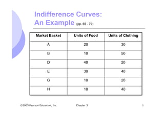
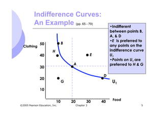
The document describes indifference curves and how they relate to consumer preferences between combinations of goods. It provides examples of indifference curves for clothing and food. Indifference curves show combinations of goods a consumer is indifferent between, and slope downward to the right since more is preferred to less. Their shape indicates how willing a consumer is to substitute one good for another. The marginal rate of substitution measures this willingness to substitute and captures the slope of the indifference curve. Perfect substitutes have a constant marginal rate of substitution, while perfect complements have right-angle shaped indifference curves. Utility and utility functions are also introduced to numerically represent satisfaction from market baskets. Budget constraints limit the combinations of goods that are affordable.

1. Chapter 3 1©2005 Pearson Education, Inc.
Indifference Curves:
An Example (pp. 65 - 79)
4010H
2010G
4030E
2040D
5010B
3020A
Units of ClothingUnits of FoodMarket Basket

2. Chapter 3 2©2005 Pearson Education, Inc.
Indifference Curves:
An Example (pp. 65 - 79)
Graph the points with one good on the x-
axis and one good on the y-axis
Plotting the points, we can make some
immediate observations about
preferences
The more, the better

3. Chapter 3 3©2005 Pearson Education, Inc.
The consumer prefers
A to all combinations
in the yellow box, while
all those in the pink
box are preferred to A.
Indifference Curves:
An Example (pp. 65 - 79)
Food
10
20
30
40
10 20 30 40
Clothing 50
G
A
EH
B
D

4. Chapter 3 4©2005 Pearson Education, Inc.
Indifference Curves:
An Example (pp. 65 - 79)
Points such as B & D have more of one
good but less of another compared to A
Need more information about consumer
ranking
Consumer may decide they are
indifferent between B, A and D
We can then connect those points with an
indifference curve

5. Chapter 3 5©2005 Pearson Education, Inc.
•Indifferent
between points B,
A, & D
•E is preferred to
any points on the
indifference curve
U1
•Points on U1 are
preferred to H & G
Indifference Curves:
An Example (pp. 65 - 79)
Food
10
20
30
40
10 20 30 40
Clothing
50
U1G
D
A
E
H
B

6. Chapter 3 6©2005 Pearson Education, Inc.
Indifference Curves (pp. 65 - 79)
Any market basket lying northeast of an
indifference curve is preferred to any
market basket that lies on the
indifference curve
Points on the curve are preferred to
points southwest of the curve

7. Chapter 3 7©2005 Pearson Education, Inc.
Indifference Curves (pp. 65 - 79)
Indifference curves slope downward to
the right
If they sloped upward, they would violate the
assumption that more is preferred to less

8. Chapter 3 8©2005 Pearson Education, Inc.
Indifference Curves (pp. 65 - 79)
To describe preferences for all
combinations of goods/services, we have
a set of indifference curves – an
indifference map
Each indifference curve in the map shows
the market baskets among which the person
is indifferent

9. Chapter 3 9©2005 Pearson Education, Inc.
U2
U3
Indifference Map (pp. 65 - 79)
Food
Clothing
U1
AB
D
Market basket A
is preferred to B.
Market basket B is
preferred to D.

10. Chapter 3 10©2005 Pearson Education, Inc.
Indifference Maps (pp. 65 - 79)
Indifference maps give more information
about shapes of indifference curves
Indifference curves cannot cross
Violates assumption that more is better
Why? What if we assume they can cross?

11. Chapter 3 11©2005 Pearson Education, Inc.
Indifference Maps (pp. 65 - 79)
Food
Clothing
•B is preferred to D
•A is indifferent to B & D
•B must be indifferent to
D but that can’t be if B is
preferred to D. A
contradiction
•Other example:
On a map, two
contours never cross
each other.
U1
U1
U2
U2
A
B
D

12. Chapter 3 12©2005 Pearson Education, Inc.
Indifference Curves (pp. 65 - 79)
The shapes of indifference curves
describe how a consumer is willing to
substitute one good for another
A to B, give up 6 clothing to get 1 food
D to E, give up 2 clothing to get 1 food
The more clothing and less food a person
has, the more clothing they will give up to
get more food

13. Chapter 3 13©2005 Pearson Education, Inc.
A
B
D
E
G
-1
-6
1
1
-4
-2
1
1
Observation: The amount
of clothing given up for
1 unit of food decreases
from 6 to 1
Indifference Curves (pp. 65 - 79)
Food
Clothing
2 3 4 51
2
4
6
8
10
12
14
16

14. Chapter 3 14©2005 Pearson Education, Inc.
Indifference Curves (pp. 65 - 79)
We measure how a person trades one
good for another using the marginal rate
of substitution (MRS)
It quantifies the amount of one good a
consumer will give up to obtain more of
another good, or the individual terms of trade
From a geometric viewpoint, it is measured
by the slope of the indifference curve

15. Chapter 3 15©2005 Pearson Education, Inc.
Marginal Rate of Substitution (pp. 65
- 79)
Food
2 3 4 51
Clothing
2
4
6
8
10
12
14
16 A
B
D
E
G
-6
1
1
1
1
-4
-2
-1
MRS = 6
MRS = 2
F
CMRS
Δ
Δ−=

16. Chapter 3 16©2005 Pearson Education, Inc.
Marginal Rate of Substitution (pp. 65
- 79)
From A to B, give up 6 clothing to get 1 food.
That is,
ΔF=2-1=1, ΔC=10-16 =-6; MRS=- ΔC / ΔF=6
From D to E, , give up 2 clothing to get 1 food;
ΔF=4-3=1, ΔC=4-6 =-2; MRS =- ΔC / ΔF= 2

17. Chapter 3 17©2005 Pearson Education, Inc.
Marginal Rate of Substitution (pp. 65
- 79)
Indifference curves are convex
As more of one good is consumed, a consumer would
prefer to give up fewer units of a second good to get
additional units of the first one. As food becomes less
scarce, he/she would give up less of clothing for an
additional food.
Consumers generally prefer a balanced market
basket (preference for varieties; the Doctrine of
the Mean in a Chinese classic)

18. Chapter 3 18©2005 Pearson Education, Inc.
Marginal Rate of Substitution (pp. 65
- 79)
The MRS decreases as we move down
the indifference curve
Along an indifference curve there is a
diminishing marginal rate of substitution.
The MRS went from 6 to 4 to 1

19. Chapter 3 19©2005 Pearson Education, Inc.
Marginal Rate of Substitution (pp. 65
- 79)
Indifference curves with different shapes
imply a different willingness to substitute
[That is, an indifference map is a concept
to represent one’s preference for market
baskets.]
Two polar cases are of interest
Perfect substitutes
Perfect complements

20. Chapter 3 20©2005 Pearson Education, Inc.
Marginal Rate of Substitution (pp. 65
- 79)
Perfect Substitutes
Two goods are perfect substitutes when the
marginal rate of substitution of one good for
the other is constant
Example: a person might consider apple
juice and orange juice perfect substitutes
They would always trade 1 glass of OJ for 1
glass of Apple Juice
Find your own examples.

21. Chapter 3 21©2005 Pearson Education, Inc.
Consumer Preferences (pp. 65 - 79)
Orange Juice
(glasses)
Apple
Juice
(glasses)
2 3 41
1
2
3
4
0
Perfect
Substitutes

22. Chapter 3 22©2005 Pearson Education, Inc.
Consumer Preferences (pp. 65 - 79)
Perfect Complements
Two goods are perfect complements when
the indifference curves for the goods are
shaped as right angles
Example: If you have 1 left shoe and 1 right
shoe, you are indifferent between having
more left shoes only
Must have one right for one left. That’s why we
always get a pair of shoes, not one by one.
Find your own examples.

23. Chapter 3 23©2005 Pearson Education, Inc.
Consumer Preferences (pp. 65 - 79)
Right Shoes
Left
Shoes
2 3 41
1
2
3
4
0
Perfect
Complements

24. Chapter 3 24©2005 Pearson Education, Inc.
Consumer Preferences:
An Application (pp. 65 - 79)
In designing new cars, automobile
executives must determine how much
time and money to invest in restyling
versus increased performance
Higher demand for car with better styling and
performance
Both cost more to improve

25. Chapter 3 25©2005 Pearson Education, Inc.
Consumer Preferences:
An Application (pp. 65 - 79)
An analysis of consumer preferences
would help to determine where to spend
more on change: performance or styling
Some consumers will prefer better styling
and some will prefer better performance
In recent years we have seen more and
more SUVs on our roads. Certainly more
owners/drivers prefer SUVs to other
styles.

26. Chapter 3 26©2005 Pearson Education, Inc.
Consumer Preferences (pp. 65 - 79)
The theory of consumer behavior does
not required assigning a numerical value
to the level of satisfaction. Can you tell
the level of satisfaction from your monthly
basket?
Although ranking of market baskets is
good, sometimes numerical value is
useful

27. Chapter 3 27©2005 Pearson Education, Inc.
Consumer Preferences (pp. 65 - 79)
Utility
A numerical score (concept) representing the
satisfaction that a consumer gets from a
given market basket. The concept of utility was
born before that of consumer preference.
If buying 3 copies of Microeconomics makes
you happier than buying one shirt, then we
say that the books give you more utility than
the shirt

28. Chapter 3 28©2005 Pearson Education, Inc.
Utility (pp. 65 - 79)
Utility function
Formula that assigns a level of utility to
individual market baskets
If the utility function is
U(F,C) = F + 2C
A market basket with 8 units of food and 3 units of
clothing gives a utility of
14 = 8 + 2(3)

29. Chapter 3 29©2005 Pearson Education, Inc.
Utility - Example (pp. 65 - 79)
4 + 2(4) = 1244C
6 + 2(4) = 1446B
8 + 2(3) = 1438A
UtilityClothingFoodMarket
Basket
Consumer is indifferent between A & B and
prefers both to C.

30. Chapter 3 30©2005 Pearson Education, Inc.
Utility - Example (pp. 65 - 79)
Baskets for each level of utility can be
plotted to get an indifference curve
To find the indifference curve for a utility of
14, we can change the combinations of food
and clothing that give us a utility of 14

31. Chapter 3 31©2005 Pearson Education, Inc.
Utility - Another Example (pp. 65 - 79)
Food
10 155
5
10
15
0
Clothing
U1 = 25
U2 = 50
U3 = 100A
B
C
Basket U = FC
C 25 = 2.5(10)
A 25 = 5(5)
B 25 = 10(2.5)

32. Chapter 3 32©2005 Pearson Education, Inc.
Utility (pp. 65 - 79)
Although we numerically rank baskets and
indifference curves, numbers are ONLY for
ranking
A utility of 4 is not necessarily twice as good as
a utility of 2. A umber assigned to a utility level
DOES NOT have any meaning.
There are two types of rankings
Ordinal ranking; Ordinal Utility Function
Think of a number on your ticket when you are in a
waiting line.
Cardinal ranking; Cardinal Utility Function
Think of the total number of students in this class.

33. Chapter 3 33©2005 Pearson Education, Inc.
Budget Constraints (pp. 79 - 83)
Preferences do not explain all of
consumer behavior
Budget constraints limit an individual’s
ability to consume in light of the prices
they must pay for various goods and
services

34. Chapter 3 34©2005 Pearson Education, Inc.
Budget Constraints (pp. 79 - 83)
The Budget Line (Constraint)
Indicates all combinations of two
commodities for which total money spent
equals total income
We assume only 2 goods are consumed, so
we do not consider savings

35. Chapter 3 35©2005 Pearson Education, Inc.
The Budget Line (pp. 79 - 83)
Let F equal the amount of food
purchased, and C is the amount of
clothing
Price of food = PF and price of
clothing = PC
Then PFF is the amount of money spent
on food, and PCC is the amount of money
spent on clothing

36. Chapter 3 36©2005 Pearson Education, Inc.
ICPFP CF =+
The Budget Line (pp. 79 - 83)
The budget line then can be written:
All income is allocated to food (F) and/or clothing
(C)

37. Chapter 3 37©2005 Pearson Education, Inc.
The Budget Line (pp. 79 - 83)
Different choices of food and clothing can
be calculated that use all income
These choices can be graphed as the budget
line
Example:
Assume income of $80/week, PF = $1 and PC
= $2

38. Chapter 3 38©2005 Pearson Education, Inc.
Budget Constraints (pp. 79 - 83)
$80080G
$801060E
$802040D
$803020B
$80400A
Income
I = PFF + PCC
Clothing
PC = $2
Food
PF = $1
Market
Basket

39. Chapter 3 39©2005 Pearson Education, Inc.
C
F
P
P
F
C
Slope -
2
1
- ==
Δ
Δ
=
The Budget Line (pp. 79 - 83)
10
20
A
B
D
E
G
(I/PC) = 40
Food
40 60 80 = (I/PF)20
10
20
30
0
Clothing

40. Chapter 3 40©2005 Pearson Education, Inc.
The Budget Line (pp. 79 - 83)
As consumption moves along a budget
line from the intercept, the consumer
spends less on one item and more on the
other
The slope of the line measures the
relative cost of food and clothing
The slope is the negative of the ratio of
the prices of the two goods

41. Chapter 3 41©2005 Pearson Education, Inc.
The Budget Line (pp. 79 - 83)
The slope indicates the rate at which the
two goods can be substituted without
changing the amount of money spent
It represents exchange ratio or terms of
trade in market places.
We can rearrange the budget line
equation to make this more clear

42. Chapter 3 42©2005 Pearson Education, Inc.
The Budget Line (pp. 79 - 83)
YX
P
P
P
I
YPXPI
YPXPI
Y
X
Y
YX
YX
=−
=−
+=