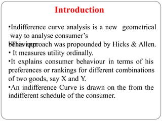
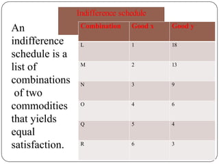
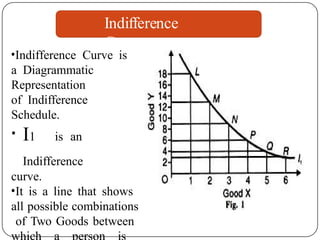
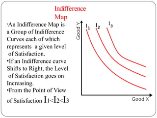
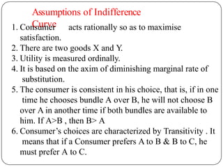
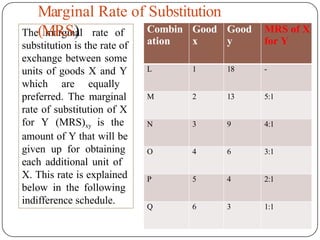
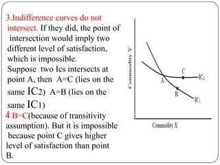
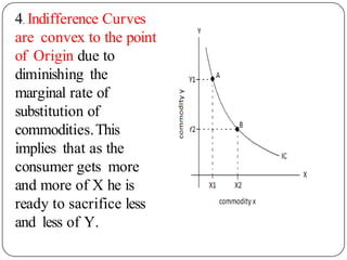
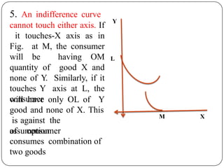
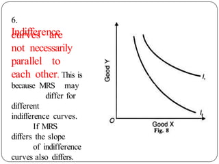
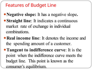
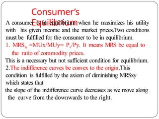
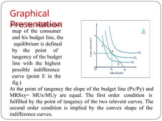
Indifference curve analysis, developed by Hicks and Allen, examines consumer behavior by representing preferences for combinations of two goods, measuring utility ordinally. An indifference curve is created from an indifference schedule, indicating all combinations that yield the same satisfaction, while properties include a negative slope, non-intersecting curves, and convexity due to diminishing marginal rate of substitution. Consumers achieve equilibrium when they maximize utility under a budget constraint, represented by the tangency of the budget line with the highest indifference curve.

1. Indifference Curve Analysis

2. Introduction
geometrical
•Indifference curve analysis is a new
way to analyse consumer’s
behaviour.
•This approach was propounded by Hicks & Allen.
• It measures utility ordinally.
•It explains consumer behaviour in terms of his
preferences or rankings for different combinations
of two goods, say X and Y.
•An indifference Curve is drawn on the from the
indifferent schedule of the consumer.

3. Indifference schedule
An
indifference
schedule is a
list of
combinations
of two
commodities
that yields
equal
satisfaction.
Combination Good x Good y
L 1 18
M 2 13
N 3 9
O 4 6
Q 5 4
R 6 3

4. Indifference
Curve
•Indifference Curve is
a Diagrammatic
Representation
of Indifference
Schedule.
• I1 is an
Indifference
curve.
•It is a line that shows
all possible combinations
of Two Goods between

5. Indifference
Map
•An Indifference Map is
a Group of Indifference
Curves each of which
represents a given level
of Satisfaction.
•If an Indifference curve
Shifts to Right, the Level
of Satisfaction goes on
Increasing.
•From the Point of View
of Satisfaction I1<I2<I3

6. Assumptions of Indifference
Curve
1. Consumer acts rationally so as to maximise
satisfaction.
2. There are two goods X and Y.
3. Utility is measured ordinally.
4. It is based on the axim of diminishing marginal rate of
substitution.
5. The consumer is consistent in his choice, that is, if in one
time he chooses bundle A over B, he will not choose B
over A in another time if both bundles are available to
him. If A>B , then B> A
6. Consumer’s choices are characterized by Transitivity . It
means that if a Consumer prefers A to B & B to C, he
must prefer A to C.

7. The marginal rate of
substitution is the rate of
exchange between some
units of goods X and Y
which are equally
preferred. The marginal
rate of substitution of X
for Y (MRS)xy is the
amount of Y that will be
given up for obtaining
each additional unit of
X. This rate is explained
below in the following
indifference schedule.
Marginal Rate of Substitution
(MRS) Combin
ation
Good
x
Good
y
MRS of X
for Y
L 1 18 -
M 2 13 5:1
N 3 9 4:1
O 4 6 3:1
P 5 4 2:1
Q 6 3 1:1

8. To have the combination M and yet to be at the same level of
satisfaction, the consumer is prepared to forgo 5 units of Y for
obtaining an extra unit of X. The marginal rate of substitution of X
for Y is 5:1. The rate of substitution will then be the number of
units of Y for which one unit of X is a substitute. As the consumer
proceeds to have additional units of X, he is willing to give away
less and less units of Y so that the marginal rate of substitution falls
from 5:1 to 1:1 in the sixth combination (Col. 4). In Fig. 8.4 above
at point M on the indifference curve I1, the consumer is willing to
give up 5 units of Y to get an additional unit of X.As he moves
along the curve form M to R, the consumer acquires more of X and
less of Y. The amount of Y he is prepared to give up to get
additional units of X becomes smaller and smaller. This behaviour
of the consumer is known as the principle of diminishing marginal
rate of substitution.

9. The marginal rate of
substitution is in fact the
slope of the curve at a
point on the indifference
curve. Thus, M.R.S. x y =
Δ Y / Δ X, on any point
on the indifference curve.
MRS Keeps on
Declining since
Consumer has more &
more units of one Good,
he gives up Less Units of
Other Good

10. Properties of Indifference
Curve
1. An Indifference Curve has a negative slope. It
denotes that if the quantity of one commodity (y)
decreases, the quantity of the other (X)
increases, if the consumer is to stay on the same
level of satisfaction. If the quantity of good X is
increased in the combination, while the quantity
of good Y remains unchanged, the new
combination will be preferable to the original
one and the two combinations will not therefore
lie on the same indifference curve provided more
of a commodity gives more satisfaction.

11. 2. A higher indifference
Curve to the right of
another represents a
higher level of
satisfaction. Here in the
fig, IC2gives more
level of satisfaction
than IC1
. This is because IC2
contains more units of
at least one
commodity

12. 3.Indifference curves do not
intersect. If they did, the point of
intersection would imply two
different level of satisfaction,
which is impossible.
Suppose two Ics intersects at
point A, then A=C (lies on the
same IC2) A=B (lies on the
same IC1)
 B=C(because of transitivity
assumption). But it is impossible
because point C gives higher
level of satisfaction than point
B.

13. 4. Indifference Curves
are convex to the point
of Origin due to
diminishing the
marginal rate of
substitution of
commodities.This
implies that as the
consumer gets more
and more of X he is
ready to sacrifice less
and less of Y.

14. 5. An indifference curve
cannot touch either axis. If
it touches-X axis as in
Fig. at M, the consumer
will be having OM
quantity of good X and
none of Y. Similarly, if it
touches Y axis at L, the
consumer
will have only OL of Y
good and none of X. This
is against the
assumption
of consumer
consumes combination of
two goods
X
L
M
Y

15. 6.
Indifference
curves are
not necessarily
parallel to
each other. This is
because MRS may
differ for
different
indifference curves.
If MRS
differs the slope
of indifference
curves also differs.

16. Exceptions of Indifference
Curve
Exception:1 If MRS of
X for Y or Y for X is
constant, the
indifference Curve will
be a straight line
sloping downwards to
the right at 45° angle to
either axis as shown in
fig. If MRS of X for Y
or Y for X is increases,
instead of diminishes,
the indifference curve
will be a concave
curve.

17. Exception:2 Perfect Complementary Goods have L-shaped
Indifference
Curves
Indifference curve of perfect
complements, as shown in Fig. A is
L-shaped (Right Angle). Perfect
complementary goods are those which
are used simultaneously in the
definite ratio for instance, right shoe
and left shoe are perfect complement
because one is useless without the
other. When consumer has its
minimum number then there is no
rate at which one shoe be substituted
for another. In case of ordinary
complementaries which have a low
rate of substitution on or near the
curvature of the curve as shown in fig
B

18. Exception 3:
Horizontal
Indifference Curve – Goods that
give zero satisfaction: When any
product yields zero satisfaction
then the consumer will not want
to sacrifice even the last quantity
of the other product to get a
single unit of that product. For
instance, indifference curve of
cigarettes for a non-smoker, as
shown in Fig., will be a straight
line. Indifference curve of that
product which yields zero
satisfaction, will be parallel to
OX (at which product yielding
zero satisfaction is shown).
O X
Y
I
C

19. Exception 4: U-Shaped
Indifference Curve Goods
that give Negative utility: If
consumption of any
product
will result in negative utility
after a certain limit, then its
indifference curve, as shown
in Fig. will be U shaped.
For instance, at point Q, the
consumer gets the quantity
of goods which are needed.
After point Q, slope of
indifference curve becomes
positive.
o x
y
I
c

20. Budget
Line
A budget line is a line which shows all combinations of two goods
that a consumer can afford with a given income and prices of
commodities It is also known as price line, consumption possibility
line, and line of attainable combinations.
Example of Budget Line
Suppose a consumer has an income of Rs.50, and it will be used to
buy commodities X andY
.To derive maximum utility from the said
income, only the following options are available.

21. Combination Goods X
(Rs 10
each)
Goods Y
(Rs 5
each)
Income (budget
allocation)
A 0 10 (10×0)+(5×10)=50
B 1 8 (10×1)+(5×8)=50
C 2 6 (10×2)+(5×6)=50
D 3 4 (10×3)+(5×4)=50
E 4 2 (10×4)+(5×2)=50
F 5 0 (10×5)+(5×0)=50

22. required
The
budget line
is obtained
by
plotting
the above
against
budget
the
following
graph. In the
graph, the X-
axis represents
commodity
X, and Y-
axis represents

23. Features of Budget Line
⚫Negative slope: It has a negative slope.
⚫Straight line: It indicates a continuous
market rate of exchange in individual
combinations.
⚫Real income line: It denotes the income and
the spending amount of a customer.
⚫Tangent to indifference curve: It is the
point when the indifference curve meets the
budget line. This point is known as the
consumer’s equilibrium.

24. Consumer’s
Equilibrium
A consumer is in equilibrium when he maximizes his utility
with his given income and the market prices.Two conditions
must be fulfilled for the consumer to be in equilibrium.
1. MRSx
y =MUx/MUy= Px/Py. It means MRS be equal to
the ratio of commodity prices.
This is a necessary but not sufficient condition for equilibrium.
2.The indifference curves be convex to the origin.This
condition is fulfilled by the axiom of diminishing MRSxy
which states that
the slope of the indifference curve decreases as we move along
the curve from the downwards to the right.

25. Graphical
Presentation
Given the indifference
map of the consumer
and his budget line, the
equilibrium is defined
by the point of
tangency of the budget
line with the highest
possible indifference
curve (point E in the
fig.)
At the point of tangency the slope of the budget line (Px/Py) and
MRSxy= MUx/MUy are equal. The first order condition is
fulfilled by the point of tangency of the two relevent curves. The
second order condition is implied by the convex shape of the
indifference curves.