IMAGE PROCESSING

1. EE 7730
Image Enhancement

2. Bahadir K. Gunturk 2
Image Enhancement
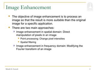
 The objective of image enhancement is to process an
image so that the result is more suitable than the original
image for a specific application.
 There are two main approaches:
 Image enhancement in spatial domain: Direct
manipulation of pixels in an image
 Point processing: Change pixel intensities
 Spatial filtering
 Image enhancement in frequency domain: Modifying the
Fourier transform of an image

3. Bahadir K. Gunturk 3
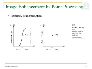
Image Enhancement by Point Processing
 Intensity Transformation

4. Bahadir K. Gunturk 4
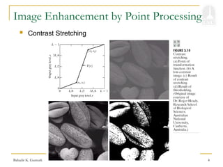
Image Enhancement by Point Processing
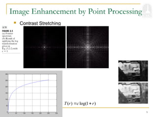
 Contrast Stretching

5. Bahadir K. Gunturk 5
Image Enhancement by Point Processing
 Contrast Stretching
( ) log(1 )
T r c r
 

6. Bahadir K. Gunturk 6
Image Enhancement by Point Processing
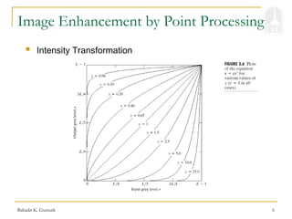
 Intensity Transformation

7. Bahadir K. Gunturk 7
Image Enhancement by Point Processing
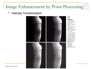
 Intensity Transformation

8. Bahadir K. Gunturk 8
Image Enhancement by Point Processing
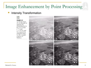
 Intensity Transformation

9. Bahadir K. Gunturk 9
Image Enhancement by Point Processing
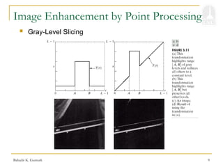
 Gray-Level Slicing

10. Bahadir K. Gunturk 12
Image Enhancement by Point Processing
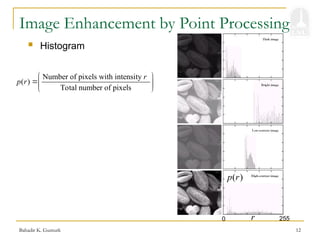
 Histogram
0 255
Number of pixels with intensity
( )
Total number of pixels
r
p r
 
 
 
( )
p r
r

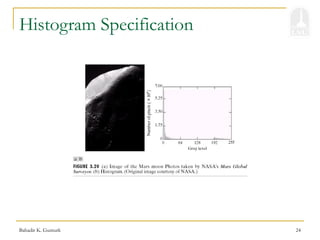
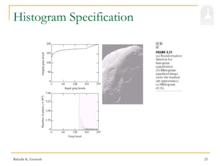
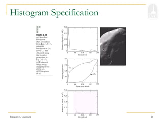
11. Bahadir K. Gunturk 13
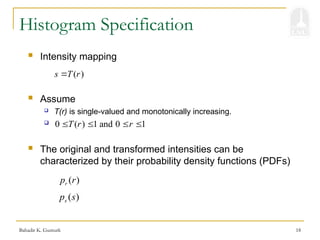
Histogram Specification
( )
s T r

 Intensity mapping
 Assume
 T(r) is single-valued and monotonically increasing.

 The original and transformed intensities can be
characterized by their probability density functions (PDFs)
0 ( ) 1 and 0 1
T r r
   
( )
r
p r
( )
s
p s

12. Bahadir K. Gunturk 14
Histogram Specification
1
( )
( ) ( )
s r
r T s
dr
p s p r
ds 

 
 
 
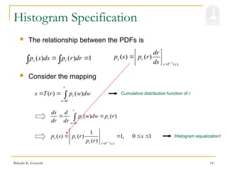
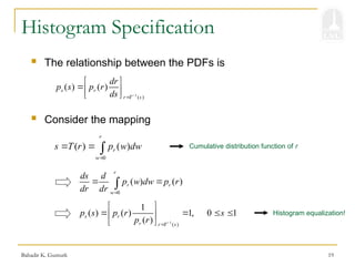
 The relationship between the PDFs is
0
( ) ( )
r
r
w
s T r p w dw

  
0
( ) ( )
r
r r
w
ds d
p w dw p r
dr dr 
 

 Consider the mapping
Cumulative distribution function of r
1
( )
1
( ) ( ) 1, 0 1
( )
s r
r r T s
p s p r s
p r 

 
   
 
 
Histogram equalization!
( ) ( ) 1
s r
p s ds p r dr
 
 

13. Bahadir K. Gunturk 15
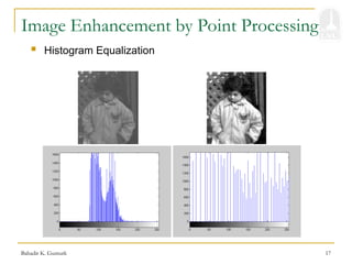
Image Enhancement by Point Processing
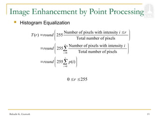
 Histogram Equalization
Number of pixels with intensity
( ) 255
Total number of pixels
i r
T r round
 

  
 
0 255
r
 
0
255 ( )
r
i
round p i

 
  
 

0
Number of pixels with intensity
255
Total number of pixels
r
i
i
round

 
  
 


14. Bahadir K. Gunturk 16
Image Enhancement by Point Processing
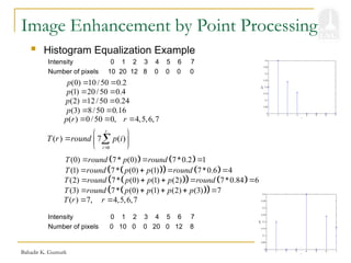
 Histogram Equalization Example
Intensity 0 1 2 3 4 5 6 7
Number of pixels 10 20 12 8 0 0 0 0
Intensity 0 1 2 3 4 5 6 7
Number of pixels 0 10 0 0 20 0 12 8
(0) 10/50 0.2
p  
(1) 20/50 0.4
p  
(2) 12/50 0.24
p  
(3) 8/50 0.16
p  
( ) 0/50 0, 4,5,6,7
p r r
  
0
( ) 7 ( )
r
i
T r round p i

 
  
 

   
(0) 7* (0) 7*0.2 1
T round p round
  
 
   
(1) 7* (0) (1) 7*0.6 4
T round p p round
   
 
   
(2) 7* (0) (1) (2) 7*0.84 6
T round p p p round
    
 
 
(3) 7* (0) (1) (2) (3) 7
T round p p p p
    
( ) 7, 4,5,6,7
T r r
 

15. Bahadir K. Gunturk 17
Image Enhancement by Point Processing
 Histogram Equalization

16. Bahadir K. Gunturk 18
Histogram Specification
( )
s T r

 Intensity mapping
 Assume
 T(r) is single-valued and monotonically increasing.

 The original and transformed intensities can be
characterized by their probability density functions (PDFs)
0 ( ) 1 and 0 1
T r r
   
( )
r
p r
( )
s
p s

17. Bahadir K. Gunturk 19
Histogram Specification
1
( )
( ) ( )
s r
r T s
dr
p s p r
ds 

 
 
 
 The relationship between the PDFs is
0
( ) ( )
r
r
w
s T r p w dw

  
0
( ) ( )
r
r r
w
ds d
p w dw p r
dr dr 
 

 Consider the mapping
Cumulative distribution function of r
1
( )
1
( ) ( ) 1, 0 1
( )
s r
r r T s
p s p r s
p r 

 
   
 
 
Histogram equalization!

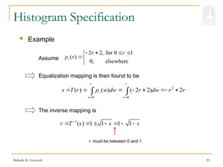
18. Bahadir K. Gunturk 20
Histogram Specification
2 2, for 0 1
( )
0, elsewhere
r
r r
p r
   



 Example
2
0 0
( ) ( ) ( 2 2) 2
r r
r
w w
s T r p w dw r dw r r
 
      
 
Assume
Equalization mapping is then found to be
1
( ) 1 1 1 1
r T s s s

      
The inverse mapping is
r must be between 0 and 1

19. Bahadir K. Gunturk 21
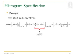
Histogram Specification
 Example
Check out the new PDF is
1
2 1 s

   
1
( ) 1 1
1
( ) ( ) ( 2 2) 1 1 2 1 1
2 1
s r
r T s r s
dr d
p s p r r s s
ds ds s

   
 
   
        
 
    
     

20. Bahadir K. Gunturk 22
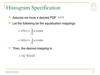
Histogram Specification
 Assume we have a desired PDF
 Let the following be the equalization mappings
( )
z
p z
0
( ) ( )
r
r
w
s T r p w dw

  
0
( ) ( )
z
z
w
v G z p w dw

  
 Then, the desired mapping is
 
1
( )
z G T r



21. Bahadir K. Gunturk 23
Histogram Specification

22. Bahadir K. Gunturk 24
Histogram Specification

23. Bahadir K. Gunturk 25
Histogram Specification

24. Bahadir K. Gunturk 26
Histogram Specification

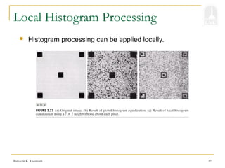
25. Bahadir K. Gunturk 27
Local Histogram Processing
 Histogram processing can be applied locally.

26. Bahadir K. Gunturk 28
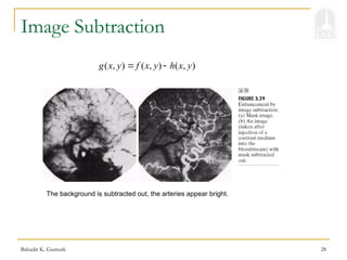
Image Subtraction
The background is subtracted out, the arteries appear bright.
( , ) ( , ) ( , )
g x y f x y h x y
 

27. Bahadir K. Gunturk 29
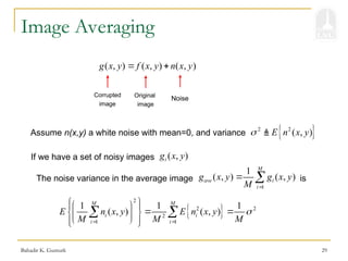
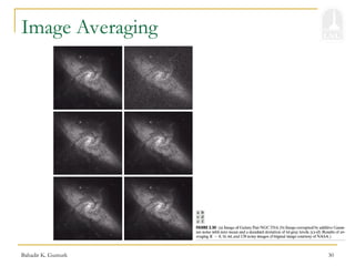
Image Averaging
( , ) ( , ) ( , )
g x y f x y n x y
 
Original
image
Noise
Corrupted
image
Assume n(x,y) a white noise with mean=0, and variance  
2 2
( , )
E n x y
 
If we have a set of noisy images ( , )
i
g x y
The noise variance in the average image is
1
1
( , ) ( , )
M
ave i
i
g x y g x y
M 
 
 
2
2 2
2
1 1
1 1 1
( , ) ( , )
M M
i i
i i
E n x y E n x y
M M M

 
 
 
 
 
 
 
 
 
 
 

28. Bahadir K. Gunturk 30
Image Averaging

29. Bahadir K. Gunturk 31
Spatial Filtering
1 1 1
1
1 1 1
9
1 1 1
 
 
 
 
 
1 1 1
1 8 1
1 1 1
 
 

 
 
 
A low-pass filter
A high-pass filter

30. Bahadir K. Gunturk 32
Spatial Filtering
 Median Filter
10 20 10
25 10 75
90 85 100
 
 
 
 
 
Sort: (10 10 10 20 25 75 85 90 100)
100 100 100 100 10 10 10 10 10
 Example
Original signal:
100 103 100 100 10 9 10 11 10
Noisy signal:
101 101 70 40 10 10 10
Filter by [ 1 1 1]/3:
100 100 100 10 10 10 10
Filter by 1x3
median filter:

31. Bahadir K. Gunturk 33
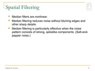
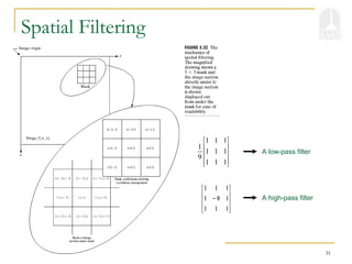
Spatial Filtering
 Median filters are nonlinear.
 Median filtering reduces noise without blurring edges and
other sharp details.
 Median filtering is particularly effective when the noise
pattern consists of strong, spikelike components. (Salt-and-
pepper noise.)

32. Bahadir K. Gunturk 34
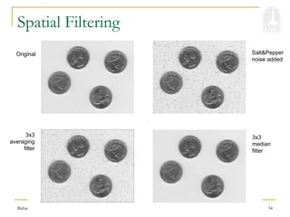
Spatial Filtering
Original
3x3
averaging
filter
Salt&Pepper
noise added
3x3
median
filter

33. Bahadir K. Gunturk 35
Spatial Filtering

34. Bahadir K. Gunturk 36
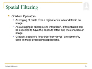
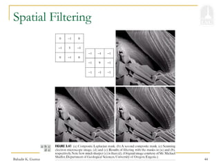
Spatial Filtering
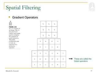
 Gradient Operators
 Averaging of pixels over a region tends to blur detail in an
image.
 As averaging is analogous to integration, differentiation can
be expected to have the opposite effect and thus sharpen an
image.
 Gradient operators (first-order derivatives) are commonly
used in image processing applications.

35. Bahadir K. Gunturk 37
Spatial Filtering
 Gradient Operators
These are called the
Sobel operators

36. Bahadir K. Gunturk 38
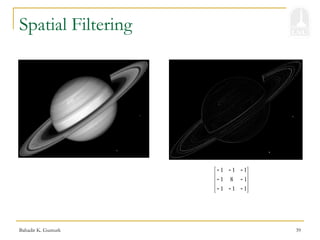
Spatial Filtering
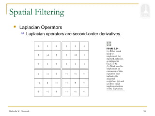
 Laplacian Operators
 Laplacian operators are second-order derivatives.

37. Bahadir K. Gunturk 39
Spatial Filtering
1 1 1
1 8 1
1 1 1
  
 
 
 
 
 
  
 

38. Bahadir K. Gunturk 40
Spatial Filtering
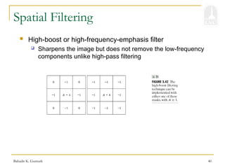
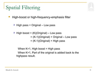
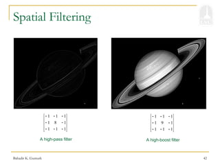
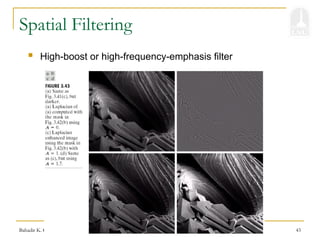
 High-boost or high-frequency-emphasis filter
 Sharpens the image but does not remove the low-frequency
components unlike high-pass filtering

39. Bahadir K. Gunturk 41
Spatial Filtering
 High-boost or high-frequency-emphasis filter
 High pass = Original – Low pass
 High boost = (K)(Original) – Low pass
= (K-1)(Original) + Original – Low pass
= (K-1)(Original) + High pass
When K=1, High boost = High pass
When K>1, Part of the original is added back to the
highpass result.

40. Bahadir K. Gunturk 42
Spatial Filtering
1 1 1
1 8 1
1 1 1
  
 
 
 
 
 
  
 
A high-pass filter A high-boost filter
1 1 1
1 9 1
1 1 1
  
 
 
 
 
 
  
 

41. Bahadir K. Gunturk 43
Spatial Filtering
 High-boost or high-frequency-emphasis filter

42. Bahadir K. Gunturk 44
Spatial Filtering