enhancement

1. EE 4780
Image Enhancement (Frequency Domain)

2. Bahadir K. Gunturk 2
Frequency-Domain Filtering
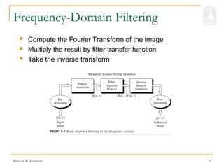
 Compute the Fourier Transform of the image
 Multiply the result by filter transfer function
 Take the inverse transform

3. Bahadir K. Gunturk 3
Frequency-Domain Filtering

4. Bahadir K. Gunturk 4
Frequency-Domain Filtering
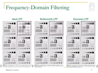
 Ideal Lowpass Filters
1, for and
( , )
0, otherwise
u v
u D v D
H u v
 



>> [f1,f2] = freqspace(256,'meshgrid');
>> H = zeros(256,256); d = sqrt(f1.^2 + f2.^2) < 0.5;
>> H(d) = 1;
>> figure; imshow(H);
Separable
Non-separable
>> [f1,f2] = freqspace(256,'meshgrid');
>> H = zeros(256,256); d = abs(f1)<0.5 & abs(f2)<0.5;
>> H(d) = 1;
>> figure; imshow(H);
2 2
0
1, for
( , )
0, otherwise
u v D
H u v

  




5. Bahadir K. Gunturk 5
Frequency-Domain Filtering
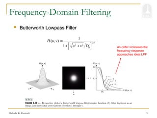
 Butterworth Lowpass Filter
2
2 2
0
1
( , )
1
n
H u v
u v D

 
 
  As order increases the
frequency response
approaches ideal LPF

6. Bahadir K. Gunturk 6
Frequency-Domain Filtering
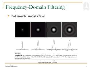
 Butterworth Lowpass Filter
Approach to a sinc function.

7. Bahadir K. Gunturk 7
Frequency-Domain Filtering
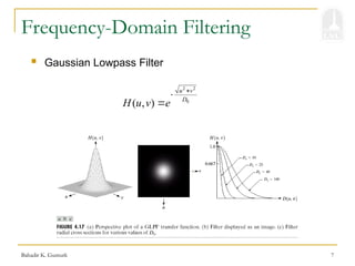
 Gaussian Lowpass Filter
2 2
0
( , )
u v
D
H u v e




8. Bahadir K. Gunturk 8
Frequency-Domain Filtering
Ideal LPF Butterworth LPF Gaussian LPF

9. Bahadir K. Gunturk 9
Example

10. Bahadir K. Gunturk 10
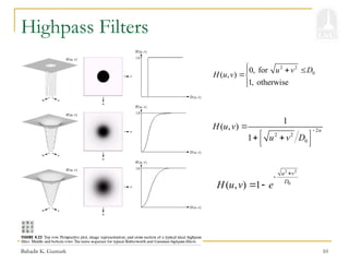
Highpass Filters
2
2 2
0
1
( , )
1
n
H u v
u v D


 
 
 
2 2
0
( , ) 1
u v
D
H u v e


 
2 2
0
0, for
( , )
1, otherwise
u v D
H u v

  




11. Bahadir K. Gunturk 11
Example

12. Bahadir K. Gunturk 12
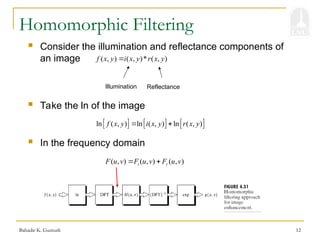
Homomorphic Filtering
 Consider the illumination and reflectance components of
an image ( , ) ( , )* ( , )
f x y i x y r x y

Illumination Reflectance
     
ln ( , ) ln ( , ) ln ( , )
f x y i x y r x y
 
 Take the ln of the image
 In the frequency domain
( , ) ( , ) ( , )
i r
F u v F u v F u v
 

13. Bahadir K. Gunturk 13
Homomorphic Filtering
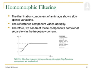
 The illumination component of an image shows slow
spatial variations.
 The reflectance component varies abruptly.
 Therefore, we can treat these components somewhat
separately in the frequency domain.
1
With this filter, low-frequency components are attenuated, high-frequency
components are emphasized.

14. Bahadir K. Gunturk 14
Homomorphic Filtering
0.5
2.0
L
H



