Ijeet 06 08_007

http://www.iaeme.com/IJEET/index.asp 63 editor@iaeme.com
International Journal of Electrical Engineering & Technology (IJEET)
Volume 6, Issue 8, Sep-Oct, 2015, pp.63-76, Article ID: IJEET_06_08_007
Available online at
http://www.iaeme.com/IJEETissues.asp?JType=IJEET&VType=6&IType=8
ISSN Print: 0976-6545 and ISSN Online: 0976-6553
© IAEME Publication
___________________________________________________________________________
REDUCTION OF SWITCHING LOSS IN
GRID-CONNECTED INVERTERS USING A
VARIABLE SWITCHING CYCLE
Tran Quang-Tho, Le Thanh-Lam, and Truong Viet-Anh
Faculty of Electrical and Electronics Engineering
Hochiminh City University of Technology and Education, Vietnam
ABSTRACT
Distributed generations (DGs) converting renewable energy sources such
as solar, wind power, and biomass into grid systems have become very
popular in the world recently. The DG using power inverter injects significant
harmonics into the grid and can cause instability of the system. Thus, the
stringent grid standards are imposed by utility companies to maintain the grid
stability. These lead to requirement of reducing current harmonics of grid-
connected inverters to achieve compliance with such grid codes. Increasing
the switching frequency of the sinusoidal pulse-width modulation (SPWM) of
inverters is a common method for reducing the total harmonic distortion
(THD) of the current; however, this increases switching losses. This paper is
to propose an SPWM technique, with a variable switching cycle in each half of
the fundamental period, for reducing the switching losses in grid-connected
inverters without increasing current harmonics. The simulation results also
validate the performance of the proposed technique compared to those of the
total demand distortion based technique and the constant ripple technique.
Key words: Electromagnetic Interference (EMI), Sinusoidal Pulse-Width
Modulation (SPWM), Switching Loss, Total Demand Distortion (TDD), Total
Harmonic Distortion (THD).
Cite this Article: Tran Quang-Tho, Le Thanh-Lam, And Truong Viet-Anh,
Reduction of Switching Loss In Grid-Connected Inverters Using A Variable
Switching Cycle. International Journal of Electrical Engineering &
Technology, 6(8), 2015, pp. 63-76.
http://www.iaeme.com/IJEET/issues.asp?JType=IJEET&VType=6&IType=8
1. INTRODUCTION
The application of DGs using renewable energy leads to a rapid development of grid-
connected inverter systems [1] toward achieving sustainable development with its
enormous potential [2]. However, grid-connected inverters insert significant current
harmonics into the power network and adversely affect the power quality of the

Tran Quang-Tho, Le Thanh-Lam, And Truong Viet-Anh
system. Thus, to meet the stringent IEEE standards 929-2000 [3] and 1547-2009 [4],
[5], harmonic reduction is considered as a primary task of engineers who design
inverter systems.
Grid-connected inverters using SPWM are widely used in renewable energy
converters [6]-[9]. Increasing an inductance of the filter is one of the popular methods
for reducing the output current harmonics; however, the size and cost of the inverters
increase as a result. Increasing the switching frequency is another method but results
in higher switching loss and the overheating of components [10].
An SPWM-based variable switching frequency technique, proposed in [11] for
reducing the switching loss of inverter, requires an accurate model of the ripple
current; additionally, the complicated calculations result in issues with robustness and
a low dynamic response. Moreover, the high ripple caused by the very low switching
frequency of the near zero current is a big drawback to digital electronic devices and
electric motors. Besides, a very high range of switching frequencies (16-90 kHz) is
not suitable for the real power semiconductor switches of grid-connected inverters
due to the limit of maximum switching frequency. Further, the performance in a grid-
connected system was also not considered in this work. Another technique using a
variable switching frequency, proposed in [12], is based on the estimated model of the
TDD. However, the filter parameter requirement and the computation time render the
performance of the method as poor in terms of the dynamic response and robustness.
A method in [13] uses an SPWM technique in which selective harmonics are
injected into the modulating signal to provide a large amount of sinusoidal
information in areas of greater sampling. Then, the modulating wave is compared to a
triangular carrier with a variable frequency over a period of the modulator. However,
the switching loss has not considered in this method. It thus is impossible to optimize
the grid-connected inverters.
Multilevel inverters in [14]-[15] are also adopted to reduce the harmonic content,
but controlling them is complicated during modulation. In addition, the excessive
numbers of power switches and DC sources increase the cost, and such equipment
suffers from problems related to capacitor voltage balance, etc. A technique proposed
in [16] to reduce the switching loss and the current THD depends on the measured
current errors and current sensors. Therefore, this method also has poor robustness.
Moreover, variable switching frequency PWM methods are usually not analyzed
quantitatively or rigorously in terms of the switching loss compared to constant
switching frequency PWM [17]-[19]. To maintain a constant root-mean-square (rms)
ripple current and to reduce the EMI noise, the switching frequency of every sector of
the space vector PWM (SVPWM) in [18] is redistributed in a nonlinearity based on
the current ripple prediction. In contrast, that of [19] is linearly increased and
decreased in each half of a sector to spread an acoustic noise spectrum and reduce
magnitudes of the dominant noise components. However, the switching loss and
application for SPWM have not been considered quantitatively.
Recently, as alternative methods instead of solving nonlinear transcendental
equations, many heuristic methods [20], such as particle swarm optimization (PSO)
[21]-[22], ant colony optimization (ACO) [23], an artificial bee colony algorithm [24],
and a genetic algorithm [25] have been proposed for eliminating selective harmonics
in SPWM; however, the switching loss has not been considered in these methods.
This paper proposes an SPWM technique, with a variable switching cycle, for
reducing the switching loss of inverters. In the proposed technique, the optimal
switching cycle of the inverter in every half of a fundamental period is determined

Reduction of Switching Loss In Grid-Connected Inverters Using A Variable Switching Cycle
improving a spread of noise spectrum in [19] for reducing the switching loss under the
constraint of current THD being equal to that of the constant switching cycle method.
The results of the implementation of a grid-connected inverter system using the
proposed method are also compared to those of the TDD method in [12] and the
constant ripple method (the hysteresis control) in [26]-[27].
2. CURRENT RIPPLE AND SWITCHING LOSS ANALYSIS
Both the current THD and switching loss of the inverter depend on the switching
frequency. In conventional SPWM techniques with a constant switching frequency, a
higher switching frequency leads to a higher switching loss and a lower current THD
and vice versa [28]. Therefore, selecting the optimal switching frequency to reduce
the switching loss without increasing the current THD of the inverter is a difficult
problem of SPWM.
To test the proposed technique, an H-bridge, grid-connected, single-phase inverter
with unipolar SPWM as in Fig. 1 is used. To analyze the current ripples, the
assumptions are made: the switching frequency of the inverter is much higher than
that of the modulated signal and the effect of dead time is negligible. The losses of the
IGBTs and diodes produce conduction, switching, and other losses. It is also assumed
that the conduction loss is not dependent on the switching frequency of the inverter
and that the switching loss linearly depends on the switched instantaneous current and
switching frequency of one switching cycle.
+
-
Vdc
~VgVi
Lf LgiL
S11
S12
S21
S22
Figure 1 H-bridge grid-connected inverter.
The inverter output current includes the fundamental current and the ripple current
based on the superposition principle.
The output current of the inverter increases in every positive half of the switching
cycle of the carrier wave and decreases in the negative half, as seen from the
waveforms in Fig. 2. In the positive half cycle of the carrier cycle, the increase in the
peak-to-peak current ripple iL1 can be calculated as
 
dc
s
f
L V
T
td
L
td
i
2
)(
)(1
1


(1)
where Lf is the inductance of the output filter of the inverter, Vdc is the DC input
voltage value of the inverter, d(t) is the duty cycle, and Ts is the cycle of the carrier
wave.
The decrease in the current ripple iL2 can be similarly calculated as
  dc
s
f
L V
T
td
L
td
i
2
)(
)(1
2 


(2)
Adding (1) and (2) for both the positive and negative half cycles of d(t) yields the
peak-to-peak current ripple as

 
dc
s
f
P V
T
td
L
td
i
2
)(
)(1

(3)
The output current waveform of the unipolar, H-bridge, single-phase inverter is
shown in Fig. 3.
Vc
t
t
t
-d
V1
iL1 iL2
ip
d
Vdc
VL Ts
Vdc-V1
-V1
i
Figure 2 Carrier wave, voltage ripple, and ripple current.
The rms value of the current ripple in each switching cycle can be defined as
)(
.32
)(1
.
3
td
L
td
VT
i
I
f
dcs
p
p




(4)
Assuming that the phase angle is ignored in this analysis. Then, the modulated signal
is expressed as
)sin(.)( tmtd  (5)
where m is the modulation index of the amplitude and  is the angular frequency of
the grid source.
Substituting (5) for d(t) into (4) yields the rms value of current ripple as
    tmtm
L
VT
I
f
dcs
p  sin..sin.1
32
.

(6)
The rms value of the current ripple in half of the fundamental period is calculated as
 




0
21
tdII p
(7)
Figure 3 Output current of inverter (m=0.97). (a) Output current and fundamental
current. (b) Current ripple.
0 0.01 0.02
-1
-0.5
0
0.5
1
(a)
(pu)
0 0.01 0.02
-0.2
0
0.2
(b)
Time (s)
(pu)
Output current
Fundamental current

The current THD has the following relation to the rms current ripple:
1I
I
THD

 (8)
where I1 is the rms value of the fundamental current.
For a constant frequency carrier wave, the switching loss is expressed as
s
sw
T
tiCP
1
.)(. 11 (9)
where the constant C1 depends on the DC voltage Vdc and i(t) is the value of the
instantaneous current flowing in the power switches. The average switching loss in
half of the fundamental period is considered to depend linearly on the switched
instantaneous fundamental current i1(t) and switching frequency in one switching
cycle. Then, the average switching loss in half of the fundamental period Psw can be
approximated as






0
1
1 )(
)sin(2
. td
T
tI
CP
s
sw (10)
3. THE PROPOSED TECHNIQUE
As mentioned above, the spread of acoustic noise spectrum in [19] for SVPWM is
used to reduce amplitude of individual harmonics. The switching cycle linearly
increases and decreases in each half of sector of SVPWM as (11) and Fig. 4, where Ts
is the fixed switching cycle. The switching frequency changes between two-third and
two of the fixed frequency in each half of sector. Fraction k is proposed to be constant
as 0.5 for all sectors.


































36
;
12
31
6
0;
12
11
)(










kT
kT
T
s
s
s
(11)
Figure 4 Switching cycle change in every sector (Ts=50s).
However, this method has not been quantitatively considered in term of switching
loss of a grid-connected inverter system. In addition, it is applied for SVPWM, not for
SPWM.
Based on the ripple description in (6), this paper proposes to improve the variable
switching cycle Tss in [19] to be suitable for the SPWM as given by (12). An
illustration for the constant frequency of 1 kHz and the fraction C3=0.5 is shown in
Fig. 5.

In (12), Tsc is a constant switching cycle, and C3 is a fraction. To improve the
performance, both Tsc and C3 are adjusted to match the load level to achieve a current
THD similar to that of the TDD method.
 












































tort
t
CT
tCT
tort
t
CT
tT
sc
sc
sc
ss
6
5
6
2
6
;
12
31
6
4
6
2
;1
6
5
6
4
6
0;
12
11
)(
3
3
3
(12)
Figure 5 Switching cycle distribution in half the fundamental period
(Tsc=1000 s; C3=0.5).
(a) Cycle. (b) Frequency.
4. SIMULATION RESULTS
The grid-connected inverter system of Fig. 1 is implemented in MATLAB/Simulink
with the parameters in Table I and the control diagram in Fig. 6. The active power
reference P_ref is stepwise varied from 3.0 kW to 1.5 kW at time t=0.2 s. The reactive
power reference Q_ref is also stepwise varied 0.0 kVar to 1.0 kVar at time t=0.35 s.
The constant C1 is defined as 2.49433x10-4
according to determination of [29].
TABLE I THE PARAMETERS OF THE SYSTEM
0 0.002 0.004 0.006 0.008 0.01
0
1
2
x 10
-3
Cycle(s)
(a)
0 0.002 0.004 0.006 0.008 0.01
0
1000
2000
(b)
Time (s)
Frequency(Hz)
Parameter Symbol Value
Inductance of filter Lf 2.5 mH
Resistance of Lf Rf 0.2 
Inductance of grid source Lg 0.01 mH
Resistance of Lg Rg 0.01 
DC voltage value Vdc 350 V
Grid source voltage Vac 220 V
Constant C1 2.494x10-4
Capacitor of filter Cf 1 µF
Fundamental frequency f 50 Hz

Figure 6 The control circuit diagram
1. The Fixed Switching Frequency of 10 kHz
Figure 7 Responses of the active and reactive powers.
Figure 8 Responses of the grid voltage and current.
I_ref
PR current controller (Kp=30&Ki=2000)
|u|2
sq1
|u|2
sq
-1
gain2
2
gain
I_error
Vdc
W
V_ref
controller
cos
Trigonometric
Function2
sin
Trigonometric
Function1
Product4
Product3
Product2
Product1
Control_signal
Carrier
S11
S21
Modulation
s21
I_error
s11
Ig
[w]
wt
I_error
Vg_max
Divide1
Car_out
Carrier
3
Vdc
2
P_ref
1
Q_ref
0 0.05 0.1 0.15 0.2 0.25 0.3 0.35 0.4 0.45 0.5
0
500
1000
1500
2000
2500
3000
3500
Power
Time (s)
Active power (W)
Reactive power (Var)
0 0.05 0.1 0.15 0.2 0.25 0.3 0.35 0.4 0.45 0.5
-30
-20
-10
0
10
20
30
Fixed cycle
Gridvoltage&current
Time (s)
Voltage/10 (V)
Current (A)

Figure 9 Switching loss and THD for the fixed cycle technique. (a) Instantaneous and
average switching loss. (b) Current THD.
2. The TDD-Based Variable Switching Frequency
Figure 10 The TDD technique. (a) Instantaneous and average switching loss. (b)
Current THD.
(a)
(b)
(c )
Fig. 11. The THD of the TDD.
(a) For t<0.2 s. (b) For 0.2<t<0.35 s.(c) For
0.35<t<0.5 s.
(a)
(b)
(c)
Fig. 12. The constant ripple THD.
(a) For t<0.2 s. (b) For 0.2<t<0.35 s.
(c) For 0.35<t<0.5 s.
0 0.05 0.1 0.15 0.2 0.25 0.3 0.35 0.4 0.45 0.5
0
10
20
30
40
50
Fixed frequency (10 kHz)
Switchingloss(W)
(a)
0 0.05 0.1 0.15 0.2 0.25 0.3 0.35 0.4 0.45 0.5
0
5
10
CurrentTHD(%) (b)
Time (s)
Inst
Aver
4.575.58
2.68
18.4515.37
30.71
0 0.05 0.1 0.15 0.2 0.25 0.3 0.35 0.4 0.45 0.5
0
20
40
TDD
Switchingloss(W)
(a)
0 0.05 0.1 0.15 0.2 0.25 0.3 0.35 0.4 0.45 0.5
0
5
10
CurrentTHD(%)
(b)
Time (s)
Inst
Aver
4.73 4.78 4.6
15.35 17.53 18.34
5 kHz 11.4 kHz 9.95 kHz
0 0.05 0.1 0.15 0.2 0.25 0.3 0.35 0.4 0.45 0.5
-10
0
10
Selected signal: 25 cycles. FFT window (in red): 1 cycles
Time (s)
0 1 2 3 4 5 6 7 8
x 10
4
0
0.5
1
1.5
2
Frequency (Hz)
Fundamental (50Hz) = 19.3 , THD= 4.73%
Mag(%ofFundamental)
0 0.05 0.1 0.15 0.2 0.25 0.3 0.35 0.4 0.45 0.5
-10
0
10
Time (s)
0 1 2 3 4 5 6 7 8
x 10
4
0
0.5
1
1.5
2
2.5
Frequency (Hz)
Mag(%ofFundamental)
0 0.05 0.1 0.15 0.2 0.25 0.3 0.35 0.4 0.45 0.5
-10
0
10
Time (s)
0 1 2 3 4 5 6 7 8
x 10
4
0
0.5
1
1.5
2
2.5
Frequency (Hz)
Mag(%ofFundamental)
0 0.05 0.1 0.15 0.2 0.25 0.3 0.35 0.4 0.45 0.5
-10
0
10
Time (s)
0 1 2 3 4 5 6 7 8
x 10
4
0
0.5
1
1.5
Frequency (Hz)
Mag(%ofFundamental)
0 0.05 0.1 0.15 0.2 0.25 0.3 0.35 0.4 0.45 0.5
-10
0
10
Time (s)
0 1 2 3 4 5 6 7 8
x 10
4
0
0.5
1
1.5
Frequency (Hz)
Mag(%ofFundamental)
0 0.05 0.1 0.15 0.2 0.25 0.3 0.35 0.4 0.45 0.5
-10
0
10
Time (s)
0 1 2 3 4 5 6 7 8
x 10
4
0
0.5
1
Frequency (Hz)
Mag(%ofFundamental)

3. The Constant Ripple
In the constant ripple method [26]-[27] (the hysteresis current control), the switching
cycle Ts is defined by replacing the peak-to-peak current ripple in (6) with the
constant current ripple Ip-const and solving for Ts:
    tmtmV
LI
T
dc
fconstp
s


sin..sin.1
32.



(13)
Figure 13 The constant ripple. (a) Instantaneous and average switching loss. (b)
Current THD.
4. The Proposed Technique
In the proposed technique, the switching cycle Ts and the fraction C3 are optimally
adjusted to obtain the similar current THDs to those of the TDD in the three intervals,
respectively.
In the first interval 0<t<0.2 s, the switching cycle Ts and the fraction C3 are
chosen as 200 s and 0.5, respectively. In the second interval 0.2<t<0.35 s, Ts and C3
are adjusted as 87 s and 0.25, respectively. In the last interval 0.35<t<0.5 s, Ts and
C3 are also adjusted as 98 s and 0.53, respectively.
Figure 14 The proposed technique. (a) Instantaneous and average switching loss. (b)
Current THD.
0 0.05 0.1 0.15 0.2 0.25 0.3 0.35 0.4 0.45 0.5
0
20
40
Constant ripple
Switchingloss(W)
(a)
0 0.05 0.1 0.15 0.2 0.25 0.3 0.35 0.4 0.45 0.5
0
5
10
CurrentTHD(%)
(b)
Time (s)
Inst
Aver
14.21 16.917.1
4.71 4.74 4.6
0 0.05 0.1 0.15 0.2 0.25 0.3 0.35 0.4 0.45 0.5
0
20
40
60
Proposed cycle
Switchingloss(W)
(a)
0 0.05 0.1 0.15 0.2 0.25 0.3 0.35 0.4 0.45 0.5
0
5
10
CurrentTHD(%)
(b)
Time (s)
Inst
Aver
4.71 4.79 4.71
13.65 16.14 16.8

(a)
(b)
(c )
Fig. 15. The proposed THD.
(a) For t<0.2 s. (b) For 0.2<t<0.35 s.
(c) For 0.35<t<0.5 s.
Fig. 16. The zoomed switching cycle and
loss. (a) Switching cycle. (b) For 0.19-0.2s.
(c) For 0.49-0.5s.
TABLE II SWITCHING LOSS AND CURRENT THD
Switching 0<t<0.2s 0.2s<t<0.35s 0.35s<t<0.5s
cycle Switching THD Switching THD Switching THD
Loss (W) (%) loss (W) (%) loss (W) (%)
Constant 30.71 2.68 15.37 5.58 18.45 4.57
TDD 15.35 4.73 17.53 4.78 18.34 4.60
Constant ripple 14.21 4.71 17.10 4.74 16.90 4.60
Proposed 13.65 4.71 16.14 4.79 16.80 4.71
5. DISCUSSIONS
The simulation results of the grid-connected inverter system are shown in Figs. 7-16
and Table II. The responses of the active and reactive powers are shown in Fig. 7 for
the fixed switching frequency of 10 kHz. The responses of the grid voltage and
current in Fig. 8 show that the current lags behind the voltage when both the active
and reactive powers are injected into the grid. In the first interval (0-0.2 s), with an
active power of 3 kW, the higher current results in the higher average switching loss
of 30.71 W in Fig. 9(a) and the lower current THD of 2.68% in Fig. 9(b). Conversely,
in the second interval (0.2-0.35 s), with an active power of 1.5 kW, the lower current
leads to a lower switching loss of 15.37 W and a higher current THD of 5.58% which
0 0.05 0.1 0.15 0.2 0.25 0.3 0.35 0.4 0.45 0.5
-20
-10
0
10
20
Time (s)
0 0.5 1 1.5 2 2.5 3 3.5 4 4.5 5
x 10
4
0
0.5
1
Frequency (Hz)
Mag(%ofFundamental)
0 0.05 0.1 0.15 0.2 0.25 0.3 0.35 0.4 0.45 0.5
-20
-10
0
10
20
Time (s)
0 1 2 3 4 5 6 7 8
x 10
4
0
0.5
1
Frequency (Hz)
Mag(%ofFundamental)
0 0.05 0.1 0.15 0.2 0.25 0.3 0.35 0.4 0.45 0.5
-20
0
20
Time (s)
0 1 2 3 4 5 6 7 8
x 10
4
0
0.5
1
1.5
Frequency (Hz)
Mag(%ofFundamental)
0 0.2*pi 0.4*pi 0.6*pi 0.8*pi pi
1
2
3
4
5
x 10
-4
Cycle(s)
Half of the fundamental period
(a)
Switching cycle
TDD
Constant ripple
Proposed
0.19 0.195 0.2
0
5
10
15
20
25
30
Switchingloss(W)
Time (s)
(b)
TDD
Constant ripple
Proposed
Instantaneous switching loss
Average switching loss
0.49 0495 0.5
0
10
20
30
40
50
60Switchingloss(W)
Time (s)
(c)
TDD
Constant
Proposed
Instantaneous switching loss
Average switching loss

exceeds the standard limit [4]. The reactive power of 1.0 kVar injected into the grid in
the last interval (0.35-0.5 s) causes the current to increase and the current THD to
decrease to 4.57%, which is lower than the limit; however, this increases the
switching loss to 18.45 W.
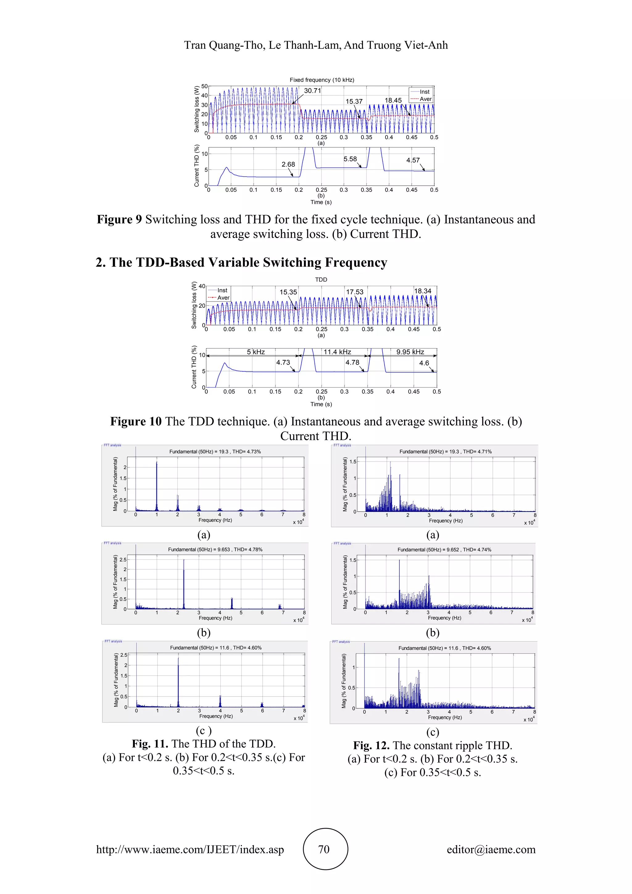
For the TDD-based variable switching frequency, the carrier frequency is changed
to reduce the switching loss in Fig. 10(b) while meeting the TDD limit (5%) specified
in [4]. To reduce the average switching loss from 30.71 W to 15.35 W to improve
efficiency in the first interval, the TDD technique must decrease the carrier frequency
from 10 kHz to 5 kHz, and the THD of 4.73% in Fig. 10(b) continues to meet the
requirement. On the other hand, the switching frequency is increased from 10 kHz to
11.4 kHz in the second interval to decrease the THD from 5.58% to 4.78%, therein
causing the switching loss to increase from 15.37 W to 17.53 W. Similarly, to reduce
the switching loss from 18.45 W to 18.34 W in the third interval, the switching
frequency is also decreased from 10 kHz to 9.95 kHz; however, this also increases the
THD from 4.57% to 4.6%. Moreover, the current spectrum in Fig. 11 shows that some
individual harmonics are still significantly high (up to 2.5%), although the THD
remains below the limit. Therefore, these harmonics can also cause some noise in
communications. In this paper, the switching loss of the TDD is chosen as the
benchmark to compare to the constant ripple technique and the proposed technique.
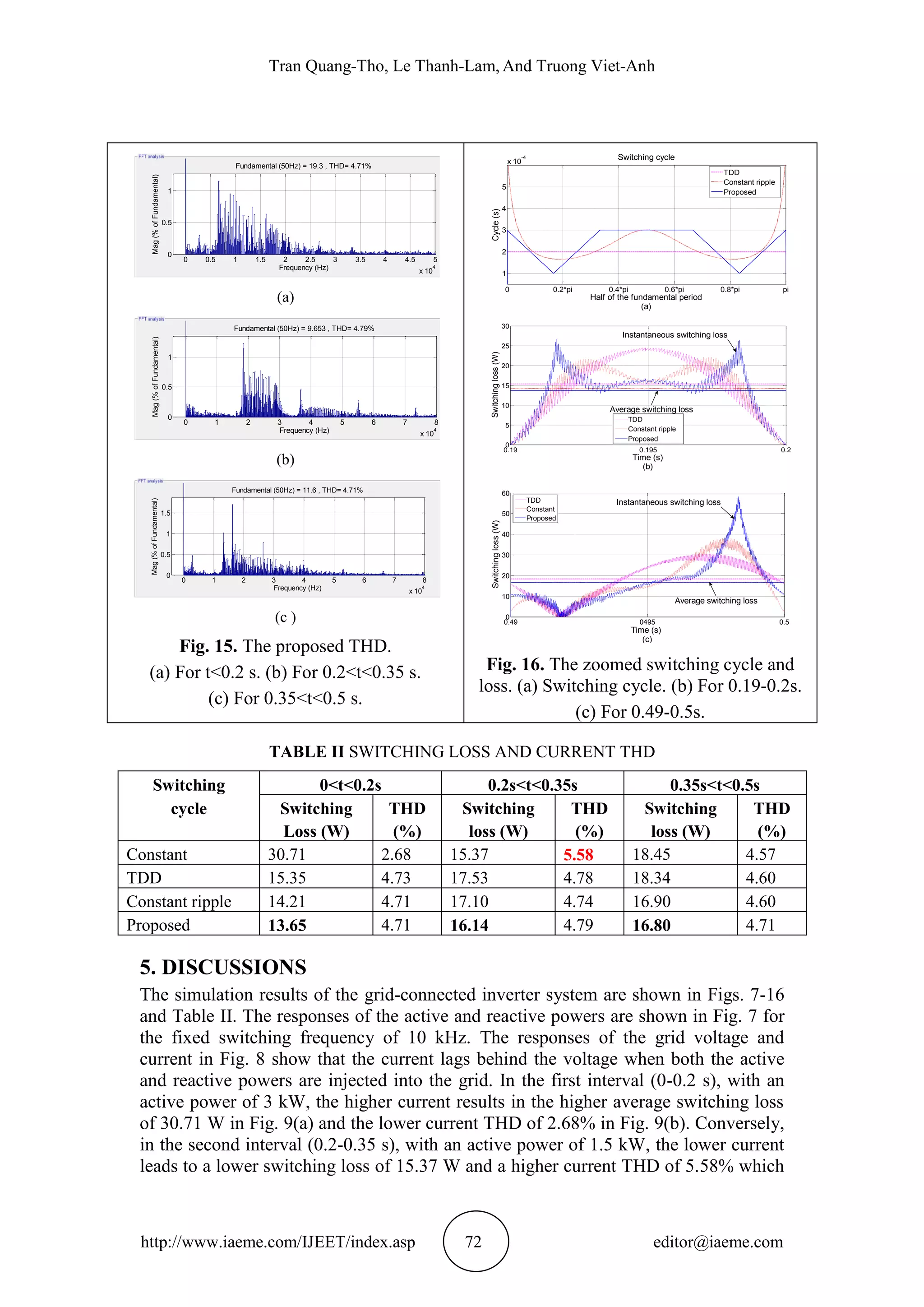
To obtain the current THDs in Fig. 13(b) similar to those of the TDD technique,
the switching loss of the constant ripple in Fig. 13(a) is equal to 14.21 W, 17.1 W, and
16.9 W in the three intervals, respectively. The spectrum of the constant ripple in Fig.
12 covers in a wide range and this leads to reducing individual harmonic amplitude
significantly.
The results of the proposed technique are shown in Figs. 14-15. With the similar
current THDs compared to those of the TDD, the average switching loss in Fig. 14(a)
is 13.65 W, 16.14 W, and 16.8 W for the three intervals, respectively. These mean
that the switching loss of the proposed technique in Table II is lower than that of the
TDD technique for the first, second, and third intervals, respectively. For the case of
unity power factor (resistance load or active power only), the instantaneous and
average switching losses in half of the fundamental period are shown in Fig. 16(b).
Similarly, for the case of non-unity power factor (R-L load or active and reactive
power), the losses are also shown in Fig. 16(c).
For the third interval, the slightly higher THD of the proposed 4.71% in Fig.15(c)
results in the slightly lower switching loss of the proposed compared to that of the
constant ripple in Table II.
The switching cycle near zero current, t=0.15, and t=0.85 of the proposed
method in Fig. 16(a) is much lower than that of the constant ripple cycle. This causes
the current ripples to be greatly reduced near zero current, whereas the instantaneous
switching loss in Figs. 16(b) and 16(c) see minimal increases. Similarly, the switching
cycle near the peak current (t=0.5), is also higher than that of the constant ripple
method. This also leads to the significant reduction in the instantaneous switching
loss, whilst the current ripples increase insignificantly. The low switching frequency
near the high instantaneous current of the proposed also contributes to increasing the
lifetime of the semiconductor devices.
6. CONCLUSIONS
Reducing the current THD of grid-connected inverters is a pressing requirement for
meeting stringent grid codes. Selecting the optimal switching cycle by striking a

balance between the switching loss and current THD is a difficult and complicated
problem.
The authors improved the spread of acoustic noise spectrum technique in [19] for
space vector PWM to SPWM to enable a suitable comparison with under the same
conditions. It is observed that by using the SPWM technique with a variable switching
cycle in every half of the fundamental period, the average switching loss can be
significantly decreased compared to what can be achieved with a constant switching
cycle. The performance of the proposed method is outstanding compared to the TDD
and constant ripple techniques, although the current THDs remain equal in all cases.
In addition, the low switching frequency of the semiconductor switches near the
peak current can help decrease the thermal stress, thus increasing the inverter’s
lifetime. The current ripple, which is significantly reduced near zero output current,
also helps improve the power quality. This enables the use of grid-connected devices
that use phase-lock loops, such as digital electronic meters and synchronization
detectors, for the recognition of phase angle and frequency to ensure proper operation.
To address the changing load currents under practical conditions, the cycle Tsc and
fraction C3 can be prepared offline for various current levels using the lookup table in
MATLAB.
The simulation results were implemented to verify the theory. For a grid-
connected inverter, operation at a non-unity power factor was also verified by
injecting the reactive power into the grid.
With the proposed technique, the current THD can be significantly reduced for the
same given switching loss. In addition, this approach can be applied to three-phase
inverters and other PWM techniques.
ACKNOWLEDGMENTS
The authors acknowledge the instrument support of Power Electronics Lab D406 and
Power System & Renewable Energy Lab C201 of HCMC University of Technology
and Education to this research project.
REFERENCES
[1] F. Blaabjerg, Z. Chen, and S. B. Kjaer, Power electronics as efficient interface in
dispersed power generation systems, IEEE Trans. Power Electron, 2004, 19(5),
1184-1194.
[2] E. Liu, and J. Bebic, Distribution system voltage performance analysis for high-
penetration photovoltaics, in GE Global Res., Niskayuna, NY, Rep. NREL/SR-
581-42298, 2008.
[3] IEEE, Recommended Practice for Utility Interface of Photovoltaic (PV) Systems,
IEEE Standard 929, 2000.
[4] IEEE, Standard for Interconnecting Distributed Resources with Electric Power
Systems, IEEE Application Guide for IEEE Standard 1547™, 2009.
[5] A. Woyte, K. De Brabandere, D. Van Dommelen, R. Belmans, and J. Nijs,
International harmonization of grid connection guidelines: adequate requirements
for the prevention of unintentional islanding, Prog. Photovolt: Res. Appl, 2003,
11(6), 407-424.
[6] T. G. Habetler and R. G. Harley, Power electronic converter and system control,
Proc. IEEE, 2001, 89(6), 913-925.

[7] Y. Sozer and D. A. Torrey, Modeling and control of utility interactive inverters,
IEEE Trans. Power Electron, 2009, 24(11), 2475-2483.
[8] L. Wu, Z. Zhao, and J. Liu, A single-stage three-phase grid-connected
photovoltaic system with modified MPPT method and reactive Power
compensation, IEEE Trans. Energy Convers, 2007, 22(4), 881-886.
[9] Z. Chen, J. M. Guerrero, and F. Blaabjerg, A review of the state of the art of
power electronics for wind turbines, IEEE Trans. Power Electron, 2009, 24(8),
1859-1875.
[10] J. H. Lee and B. H. Cho, Large time-scale electro-thermal simulation for loss and
thermal management of power MOSFET, Proc. IEEE Power Electron. Spec.
Conf, 2003, 112–117.
[11] X. Mao, R. Ayyanar, H. K. Krishnamurthy, and K. Harish, Optimal variable
switching frequency scheme for reducing switching loss in single-phase inverters
based on Time-domain ripple analysis, IEEE Trans. Power Electron, 2009, 24(4),
991-1001.
[12] B. Cao and L. Chang, A variable switching frequency algorithm to improve the
Total efficiency of single-phase grid-connected inverters, Proc. IEEE, 2013,
2310-2315.
[13] F. Perez-Hidalgo, F. Vargas-Merino, J. Heredia-Larrubia, M. Meco-Gutierrez,
and A. Ruiz-Gonzalez, Pulse width modulation technique parameter selection
with harmonic injection and frequency-modulated triangular carrier, IET Power
Electron, 2013, 6(5), 954-962.
[14] H. Iman-Eini, M. Bakhshizadeh, and A. Moeini. 2014, Selective harmonic
mitigation-pulse-width modulation technique with variable DC-link voltages in
single and three-phase cascaded H-bridge inverters, IET Power Electron, 2014,
7(4), 924–932.
[15] I. Colak, E. Kabalci, and R. Bayindir, Review of multilevel voltage source
inverter topologies and control schemes, Energ. Convers. Manag, 2011, 52(2),
1114–1128.
[16] C. Xiaoju, Z. Hang, and Z. Jianrong, A new improvement strategy based on
hysteresis space vector control of grid-connected inverter, in Proc. Int. Conf. on
Advanced Power System Automation and Protection, 2011, 1613-1617.
[17] K. Kim, Y. Jung, and Y. Lim, A new hybrid random PWM scheme, IEEE Trans.
Power Electron, 2009, 24(1), 192–200.
[18] D. Jiang and F. Wang, Variable switching frequency PWM for three-phase
converters based on current ripple prediction, IEEE Trans. Power Electron, 2013,
28(11), 4951–4961.
[19] A. C. Binojkumar and G. Narayanan, Variable switching frequency PWM
technique for induction motor drive to spread acoustic noise spectrum with
reduced current ripple, Proc. IEEE, 2014, 1-6.
[20] A. Amjad and Z. Salam, A review of soft computing methods for harmonics
elimination PWM for inverters in renewable energy conversion systems,
Renewable Sustain. Energ. Rev, 2014, 33, 141–153.
[21] R. N. Ray, D. Chatterjee, and S. K. Goswami, A PSO based optimal switching
technique for voltage harmonic reduction of multilevel inverter, Expert Syst.
Appl, 2010, 37(12), 7796–7801.
[22] T. Shindo, T. Kurihara, H. Taguchi, and K. Jin’no, Particle swarm optimization
for single phase PWM inverters, in Proc. Evolutionary Computation (CEC)-IEEE
Congress, 2011, 2501-2505.

[23] K. Sundareswaran, K. Jayant, and T. N. Shanavas, Inverter harmonic elimination
through a colony of continuously exploring ants, IEEE Trans. Ind. Electron,
2007, 54(5), 2558–2565.
[24] A. Kavousi, B. Vahidi, R. Salehi, M. K. Bakhshizadeh, N. Farokhnia, and S. H.
Fathi, Application of the bee algorithm for selective harmonic elimination
strategy in multilevel inverters, IEEE Trans. Power Electron, 2012, 27(4), 1689–
1696.
[25] K. L. Shi and H. Li, Optimized PWM strategy based on genetic algorithms, IEEE
Trans. Ind. Electron, 2005, 52(5), 1458–1461.
[26] J. Holtz, Pulse width modulation-a survey, IEEE Trans. Ind. Electron, 1992,
39(5), 410–420.
[27] F. Zare and A. Nami, A new random current control technique for a single-phase
inverter with bipolar and unipolar modulations, Proc. IEEE, 2007, 149–156.
[28] R. Seyezhai and B. L. Mathur, Performance evaluation of inverted Sine PWM
technique for an asymmetric cascaded multilevel inverter, J. Theor. Appl. Inf.
Technol, 2009, 9(2), 91-98.
[29] T. Q. Tho, L. T. Lam, T. N. Trieu, and T. V. Anh, PWM Technique Using
Variable Switching Frequency To Reduce Current THD In Grid-Connected
Inverters, Mitteilungen Klosterneuburg, 2015, 65(4), 354-367.
[30] Haider M. Husen , Laith O. Maheemed, Prof. D.S. Chavan, Enhancement of
Power Quality In Grid-Connected Doubly Fed Wind Turbines Induction
Generator. International Journal of Electrical Engineering & Technology, 3(1),
2012, pp. 182 - 196.
[31] Tran Quang Tho, Truong Viet Anh, Three-Phase Grid-Connected Inverter Using
Current Regulator. International Journal of Electrical Engineering &
Technology, 4(2), 2013, pp. 293 – 304.

Ijeet 06 08_007

More Related Content

What's hot

Viewers also liked

Similar to Ijeet 06 08_007

More from IAEME Publication

Recently uploaded

Ijeet 06 08_007