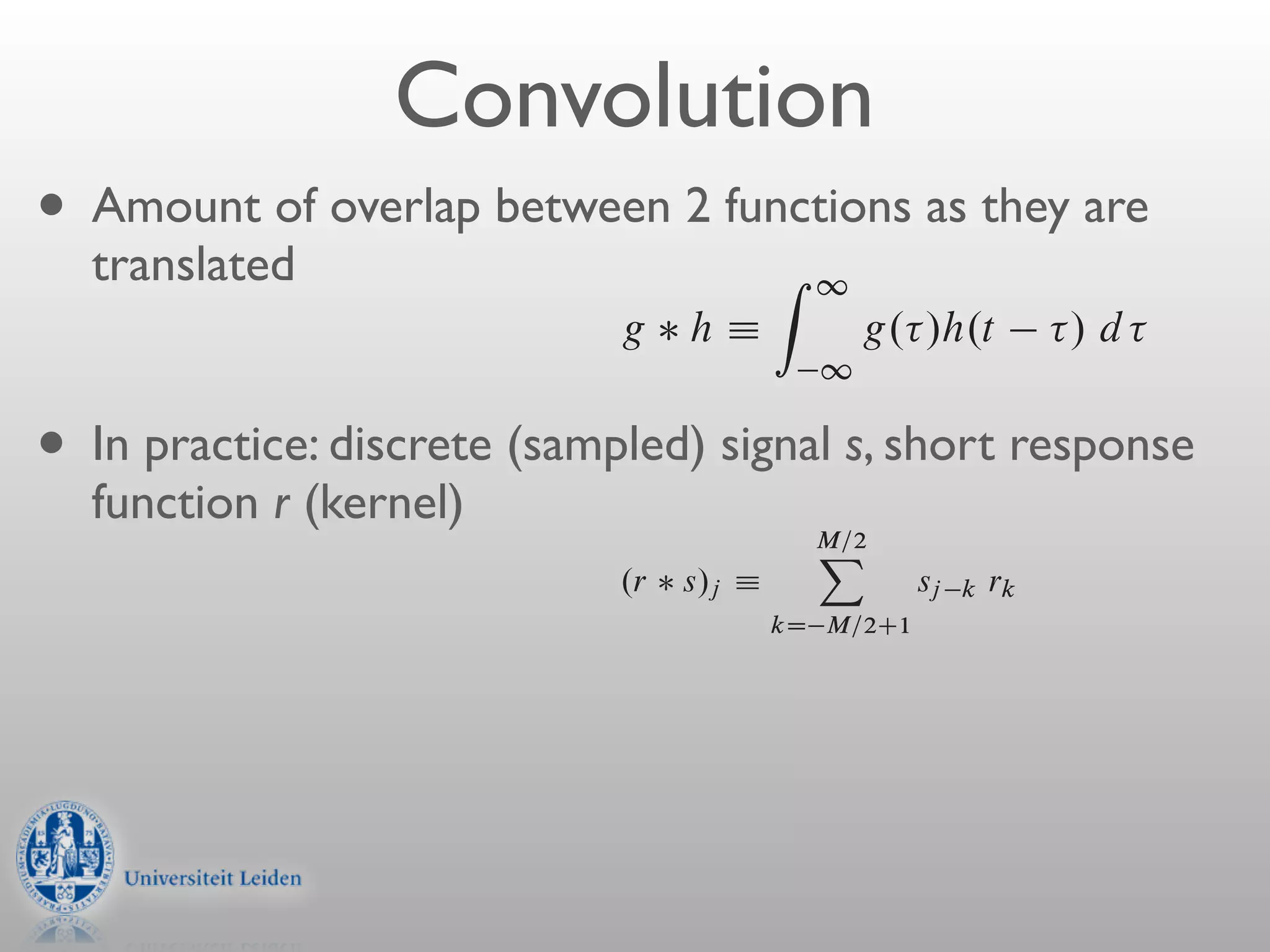
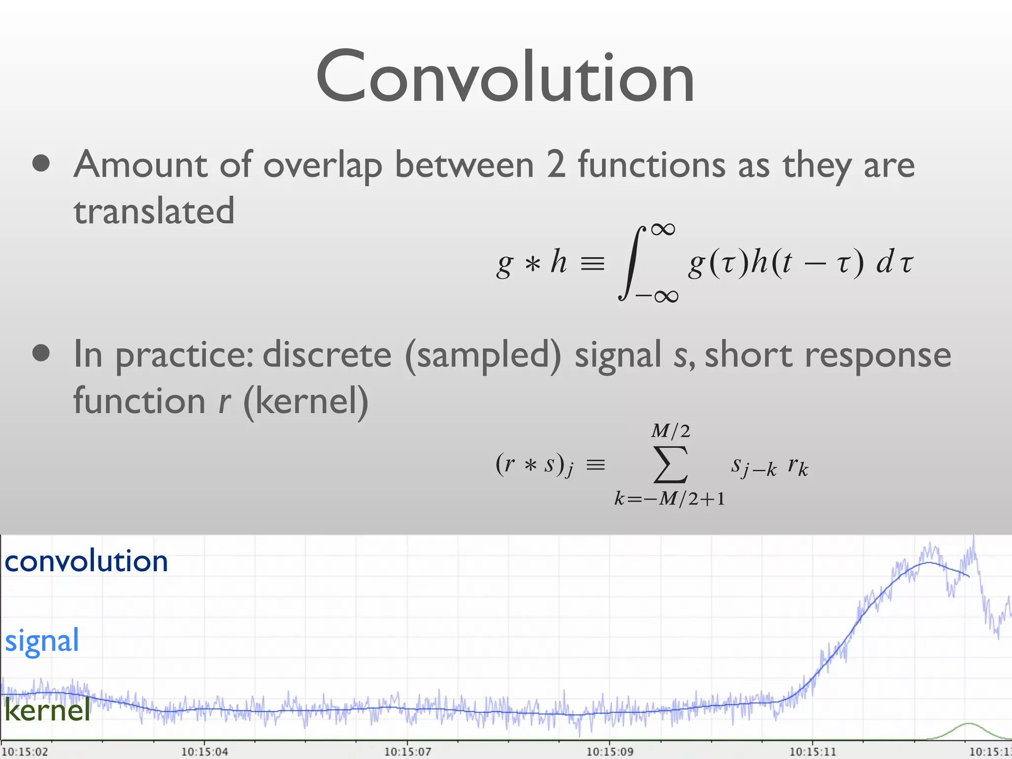
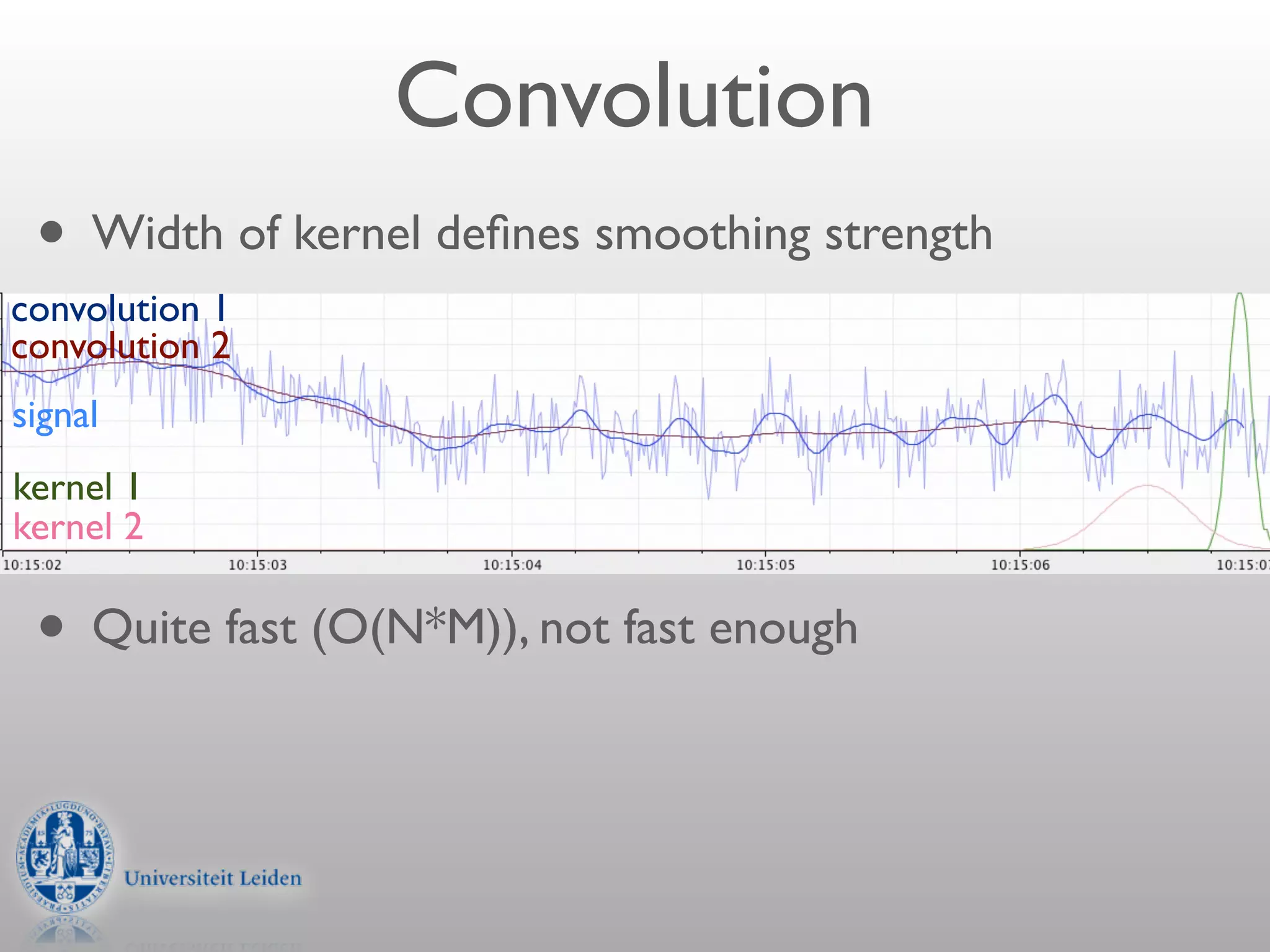
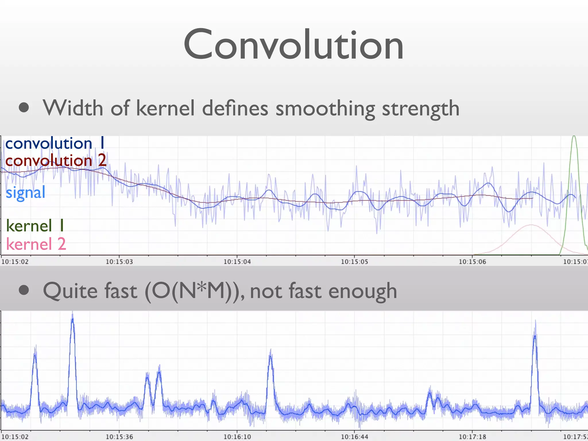
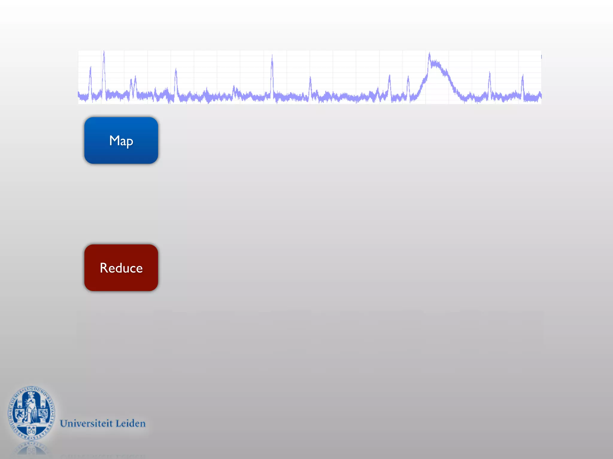
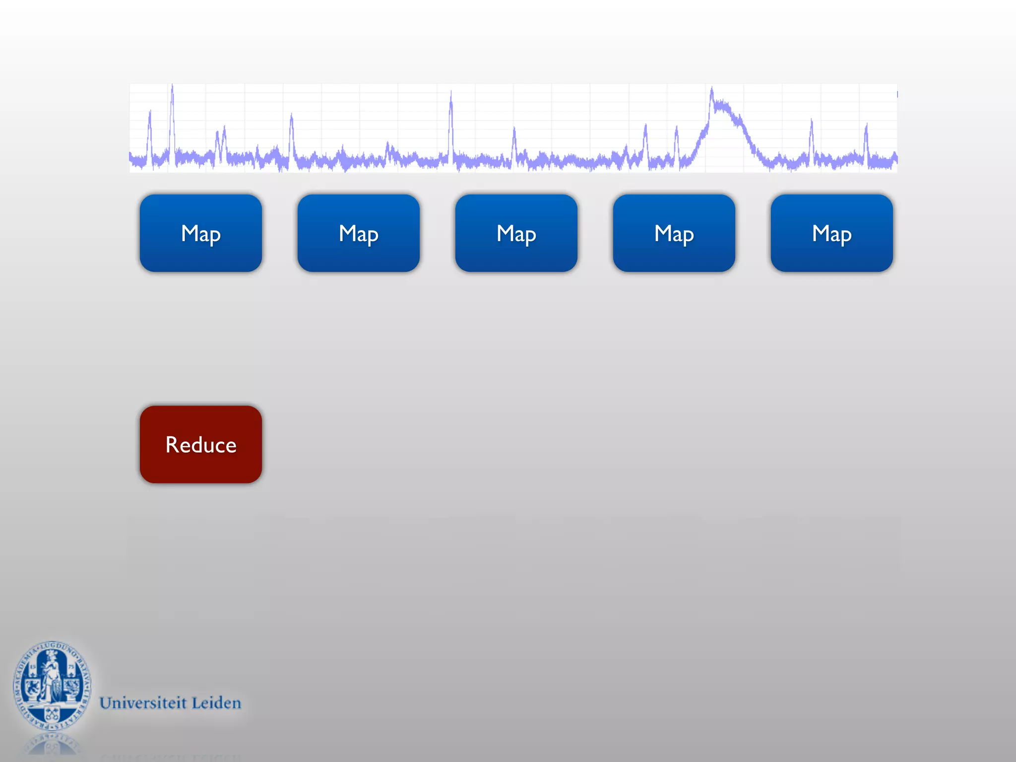
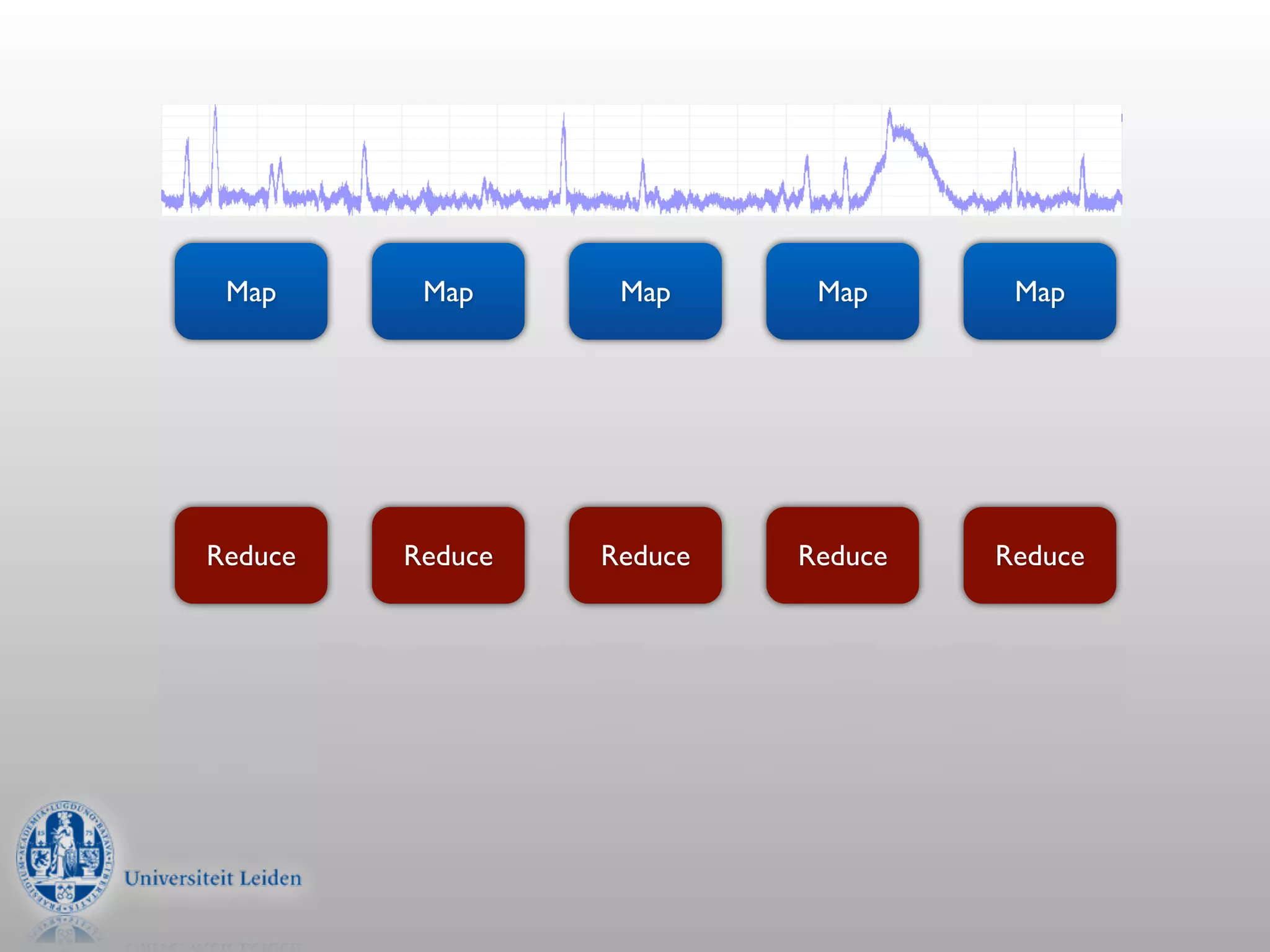
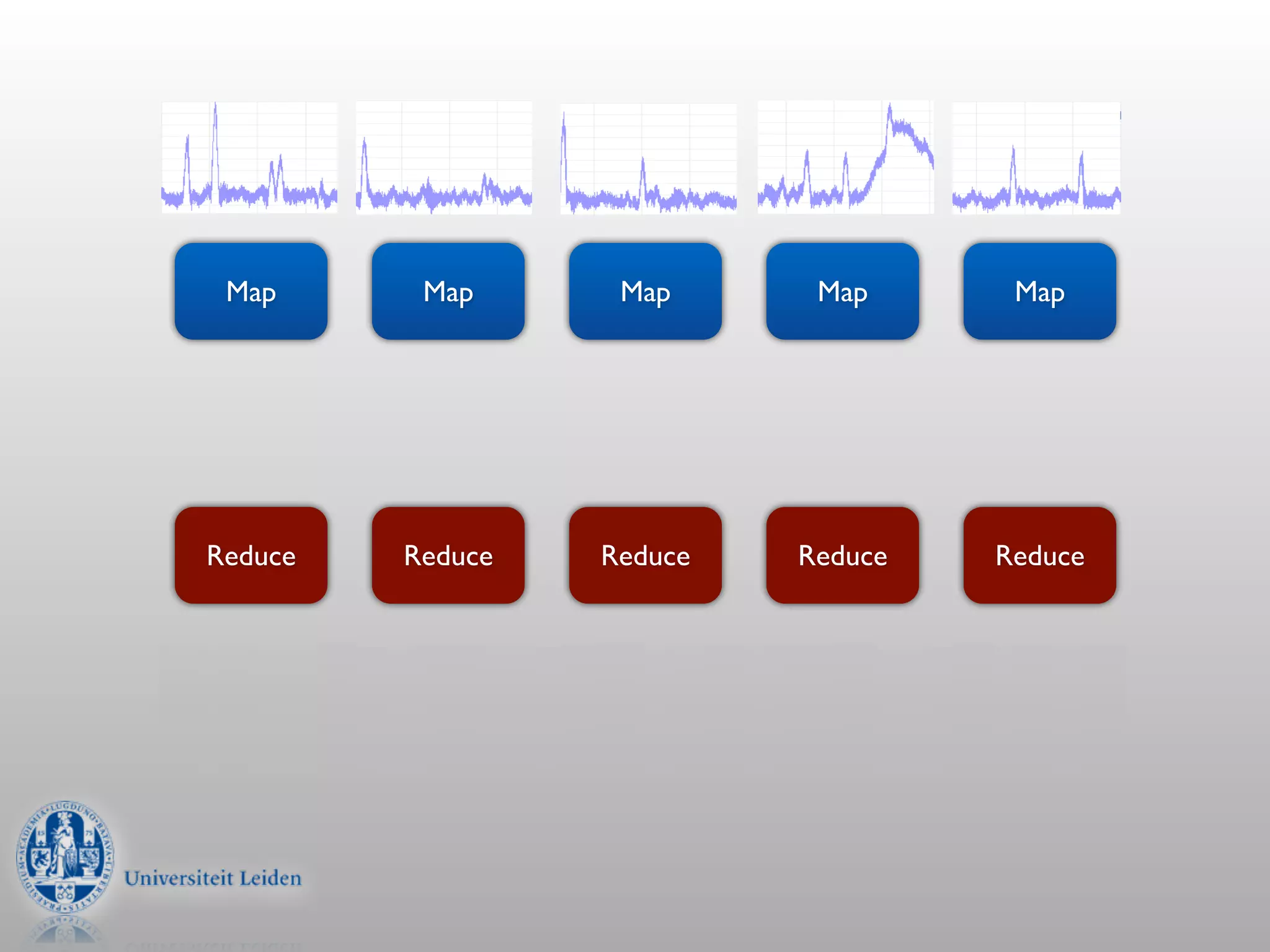
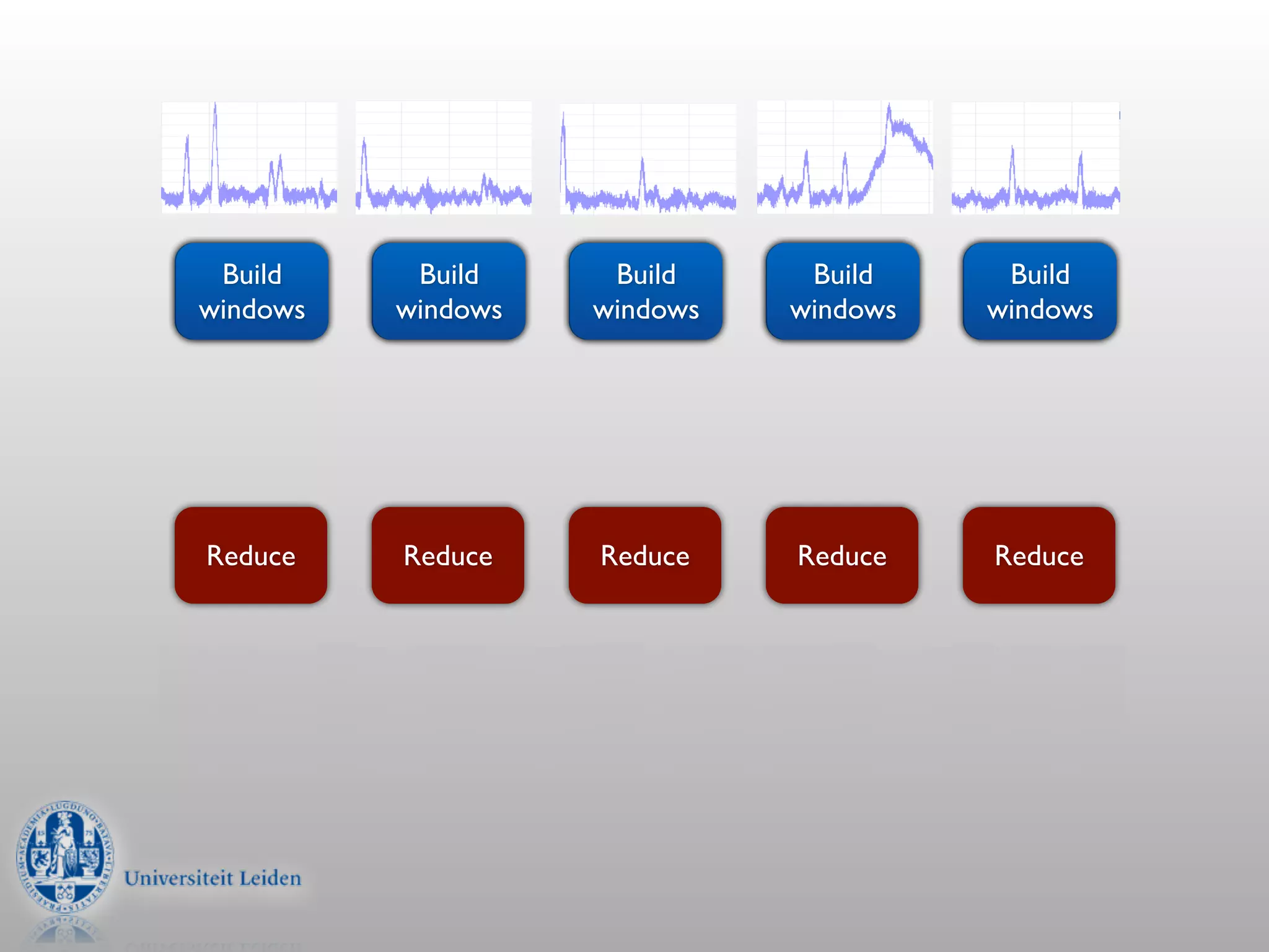
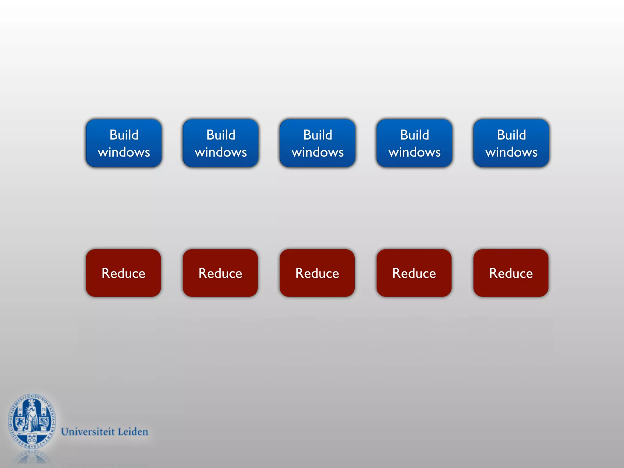
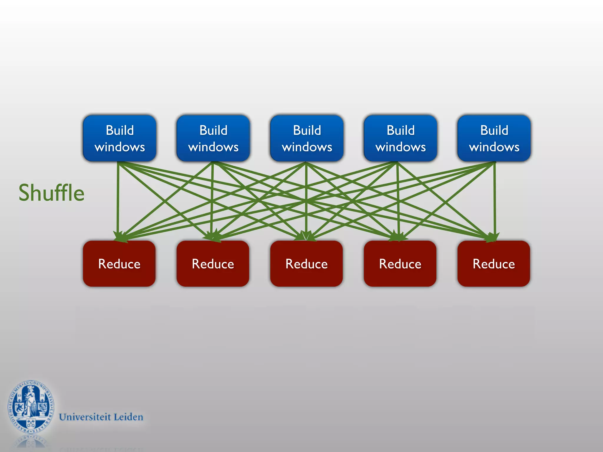
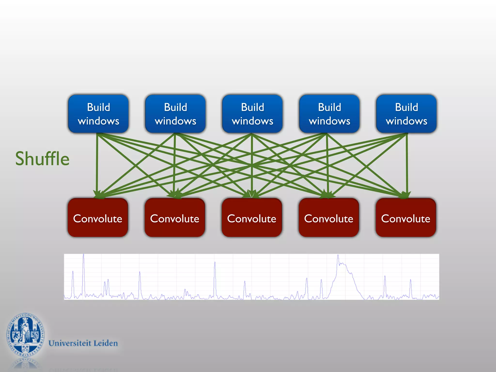
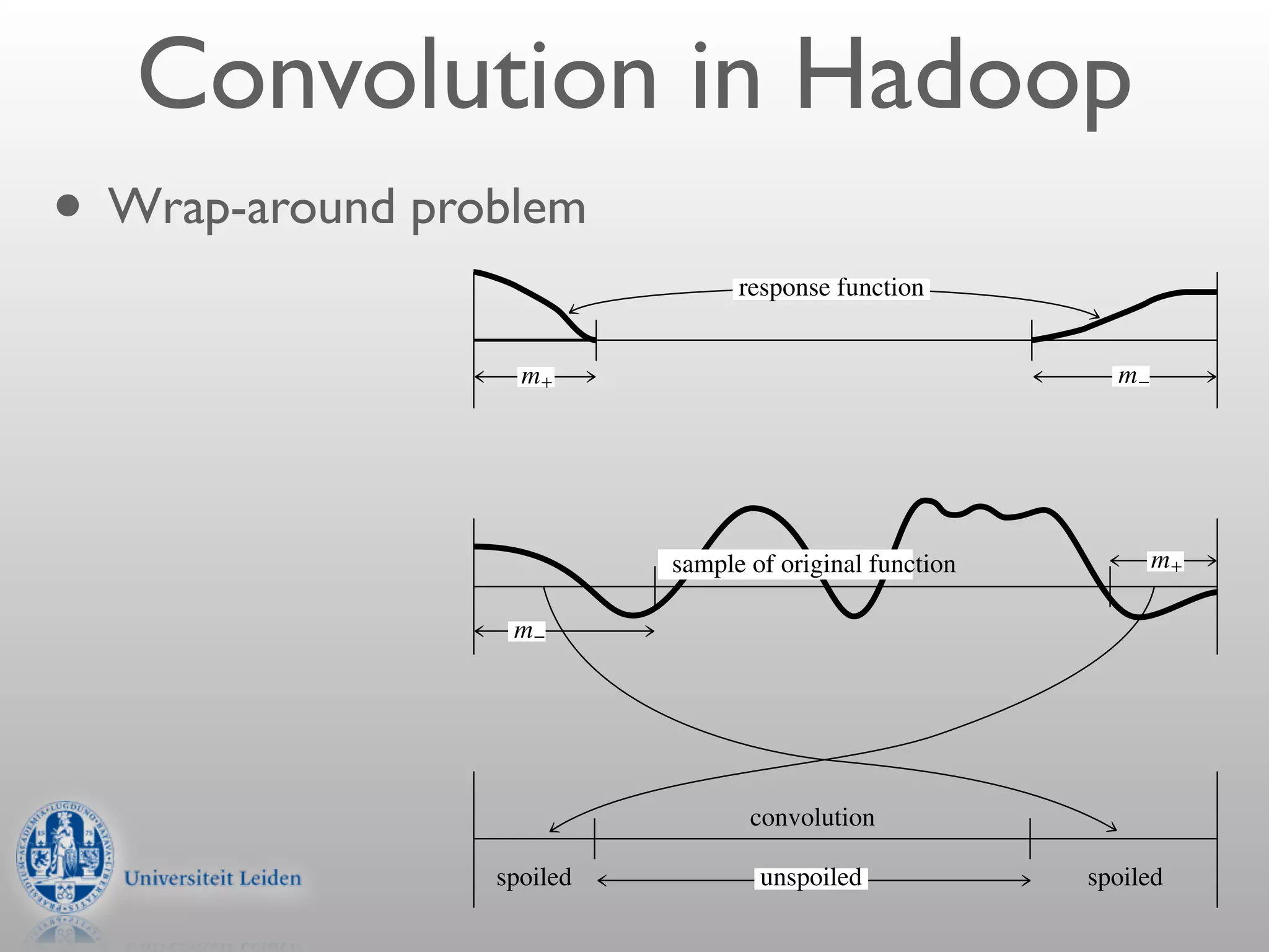
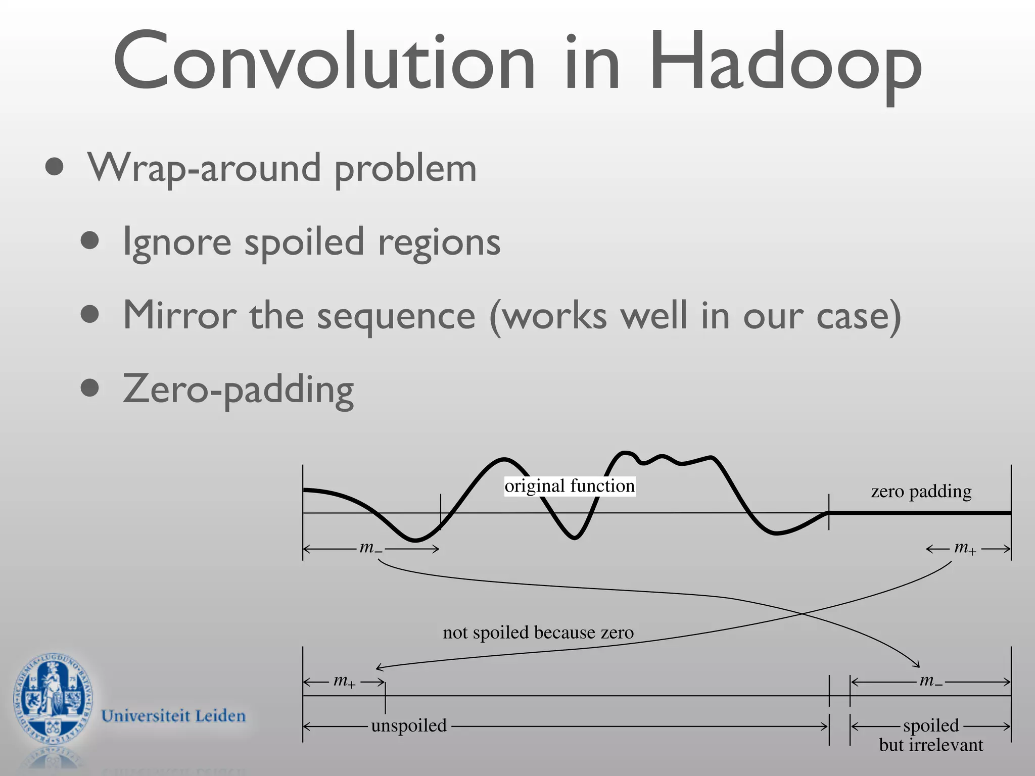
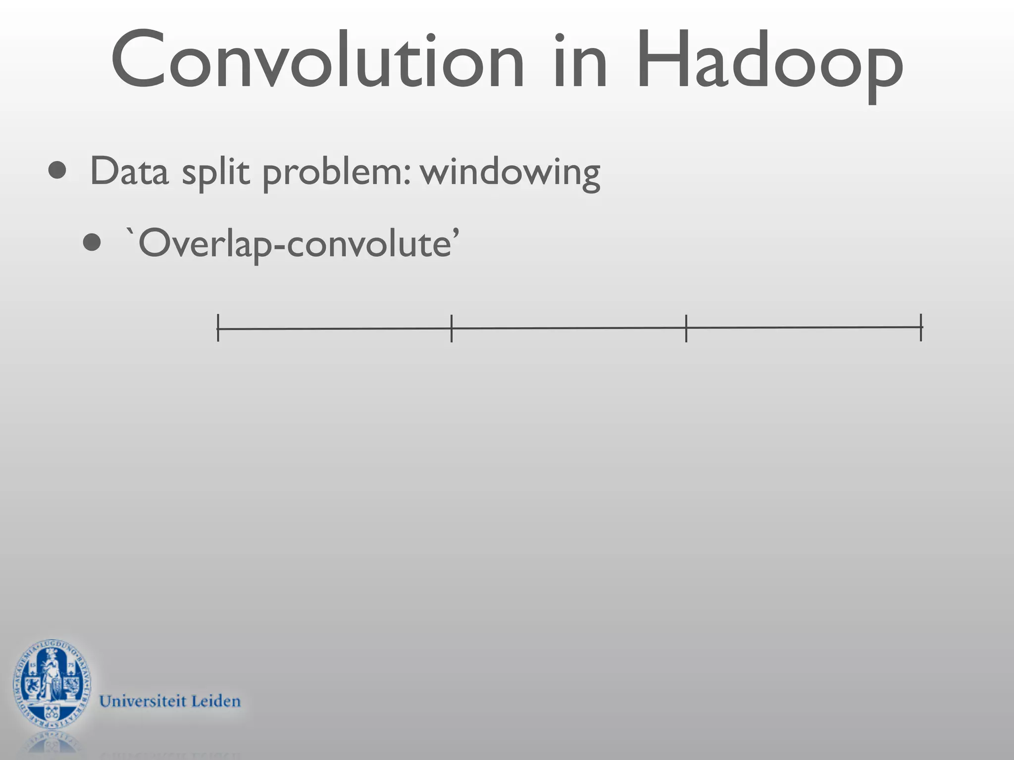
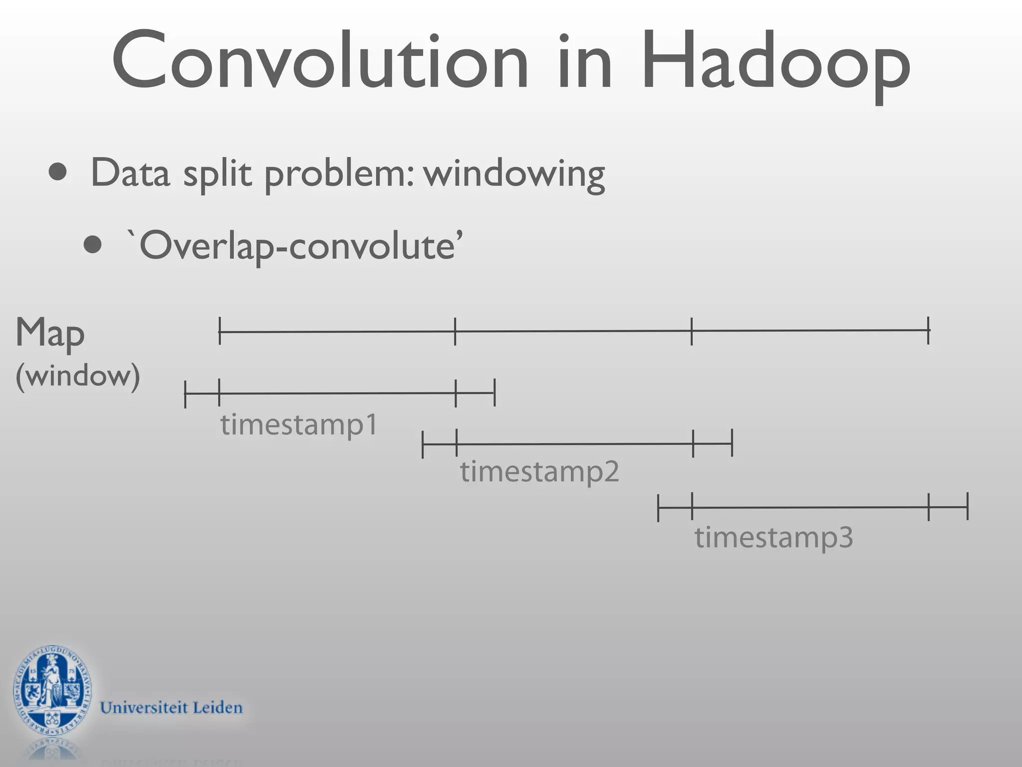
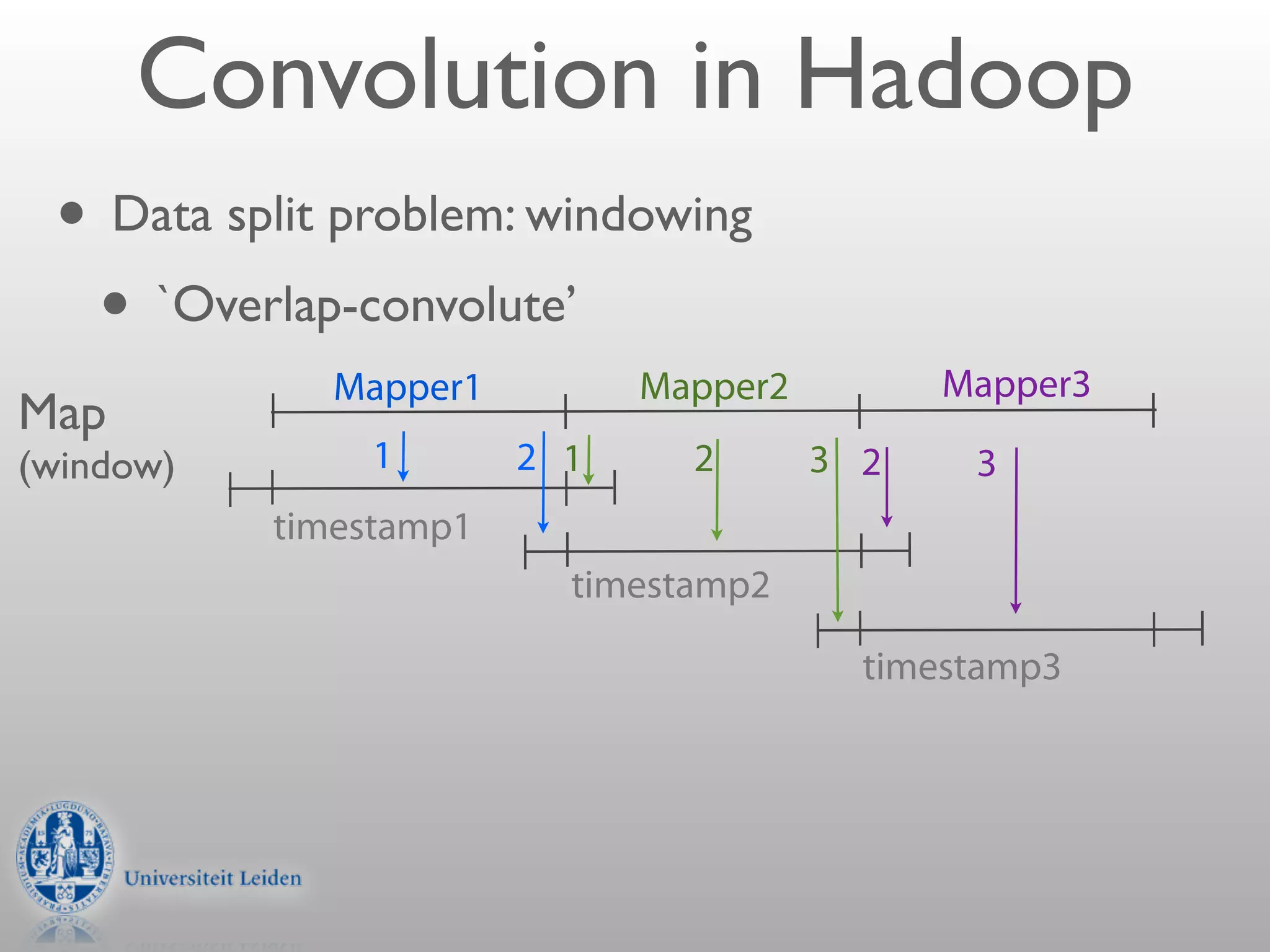
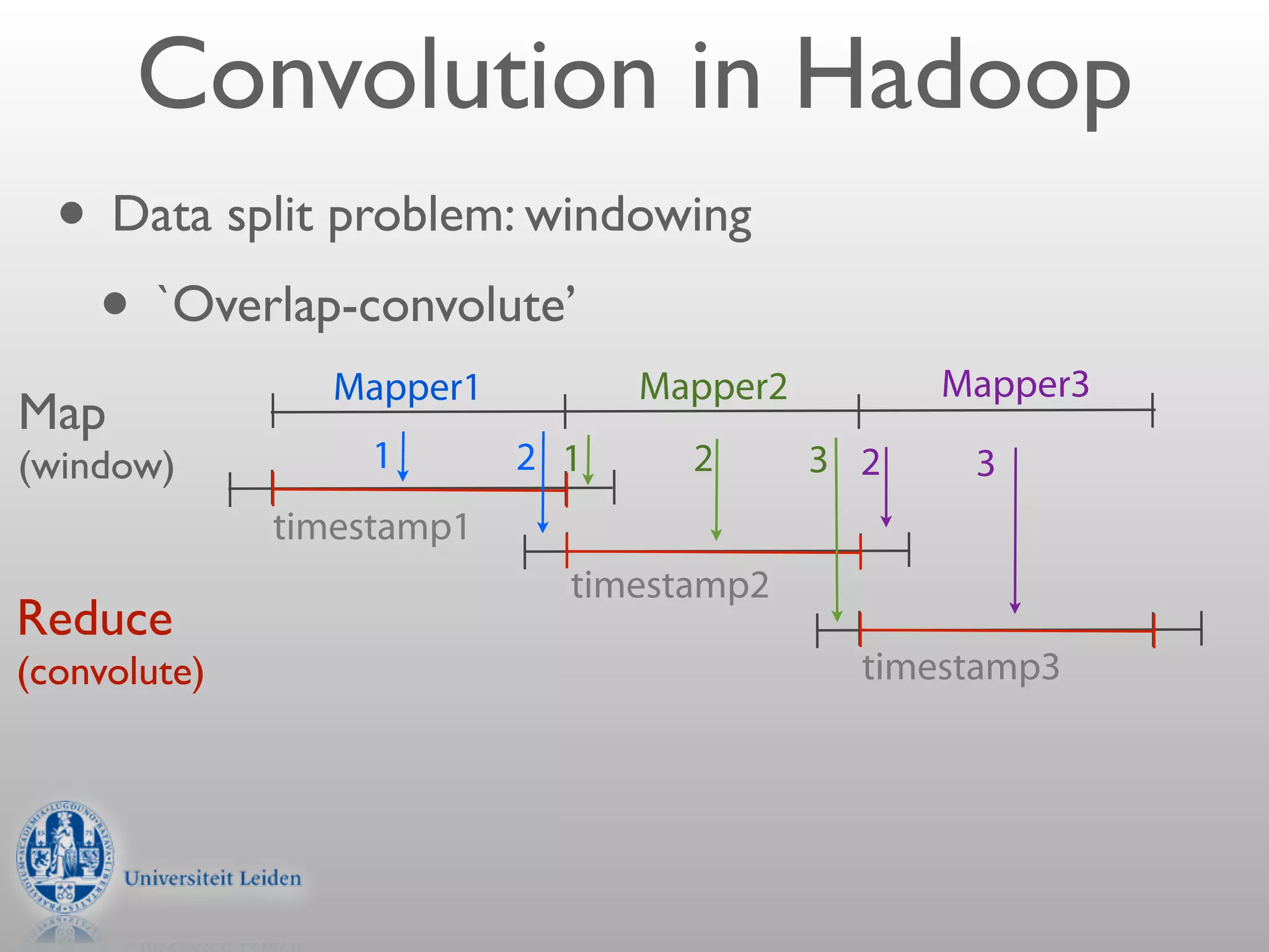
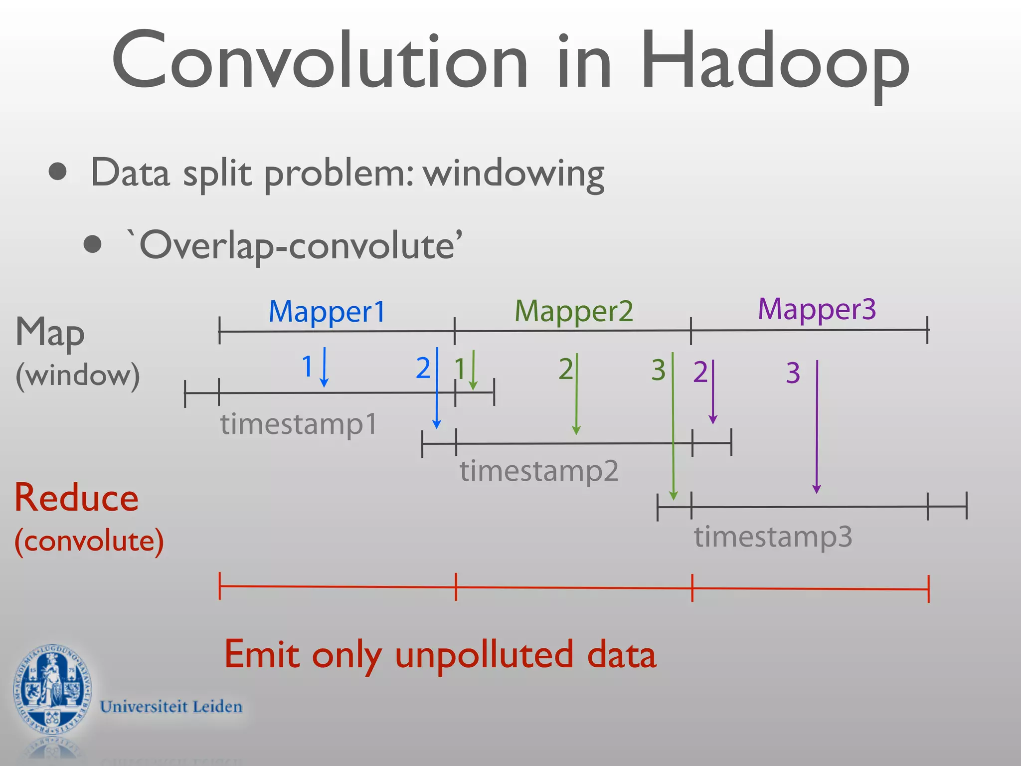
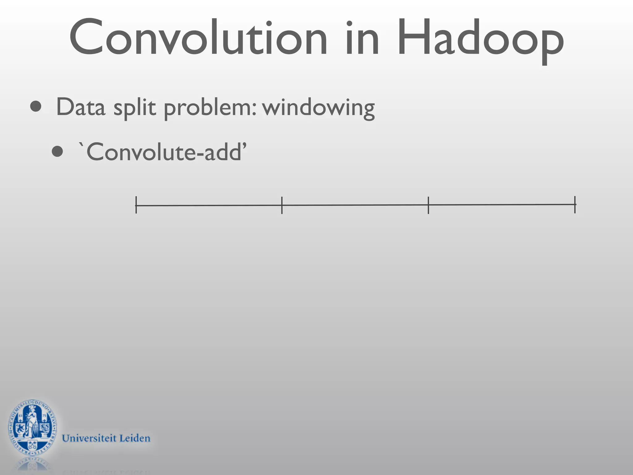
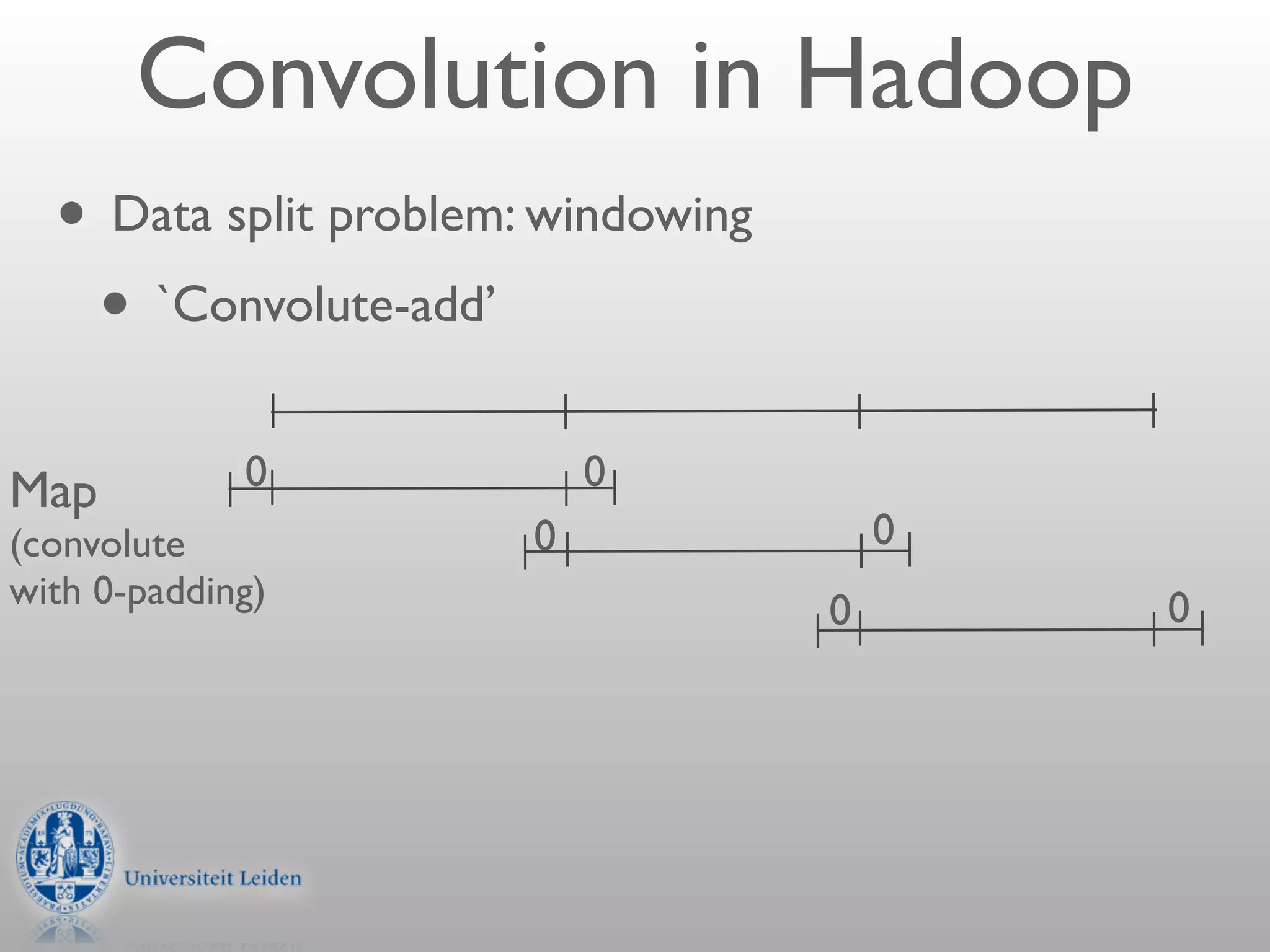
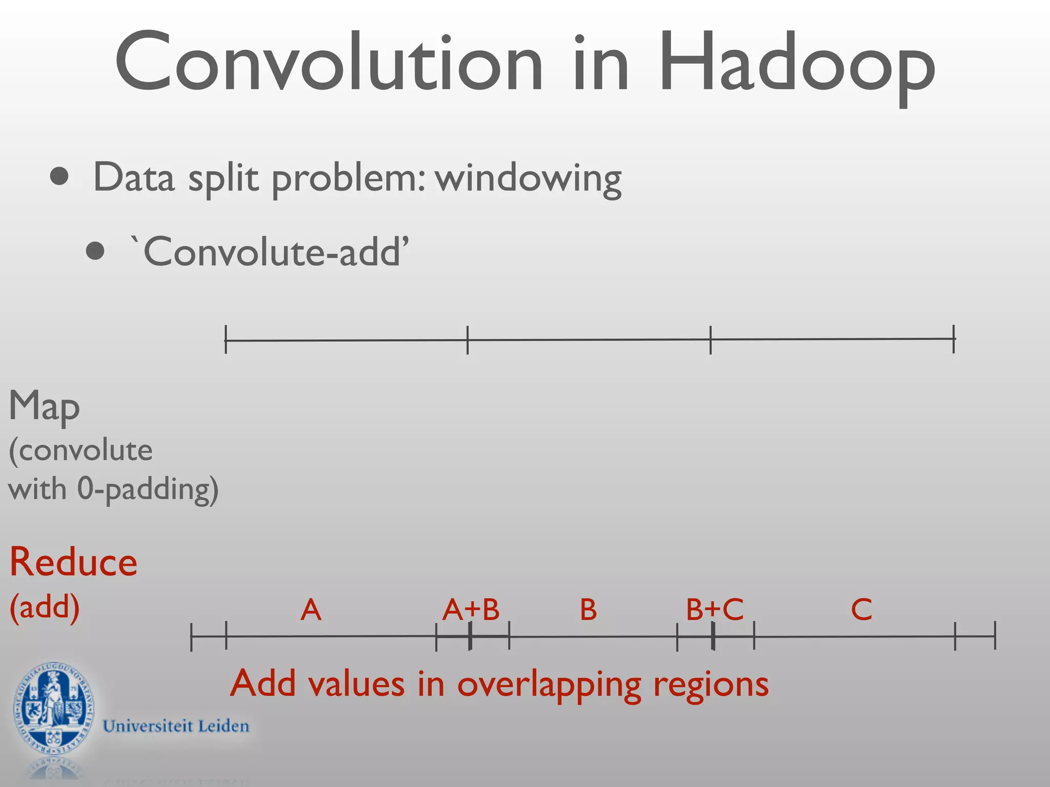
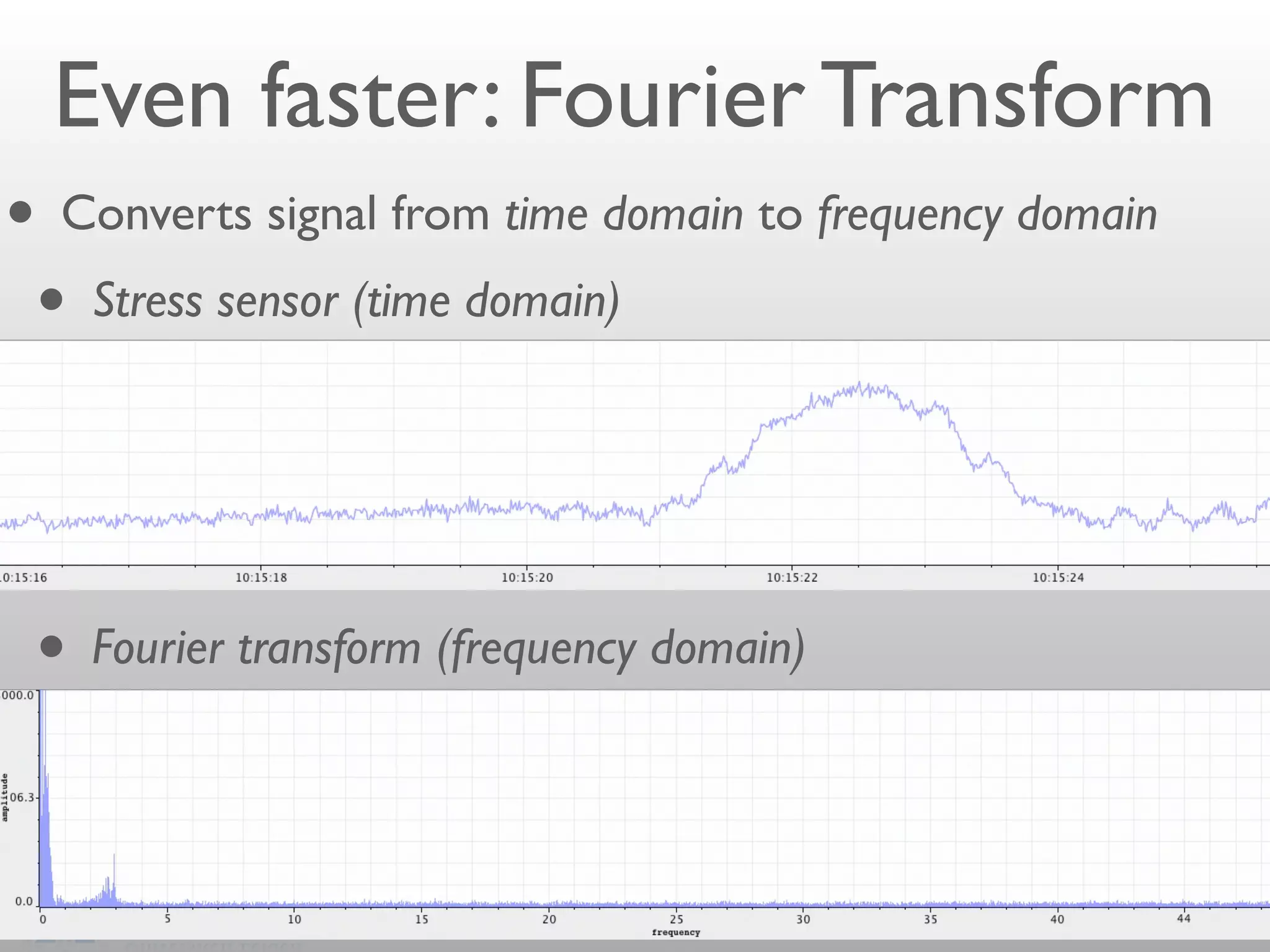
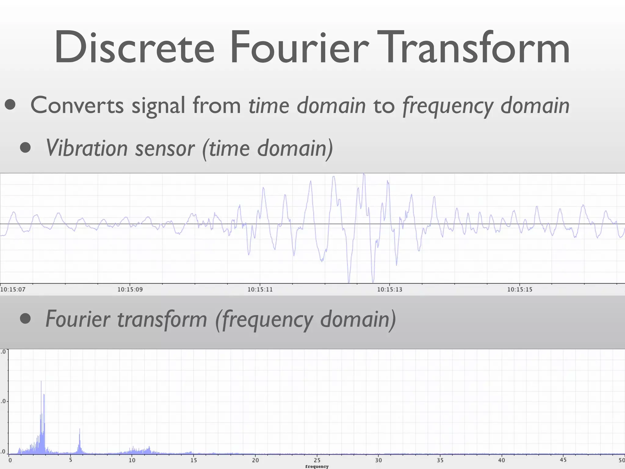
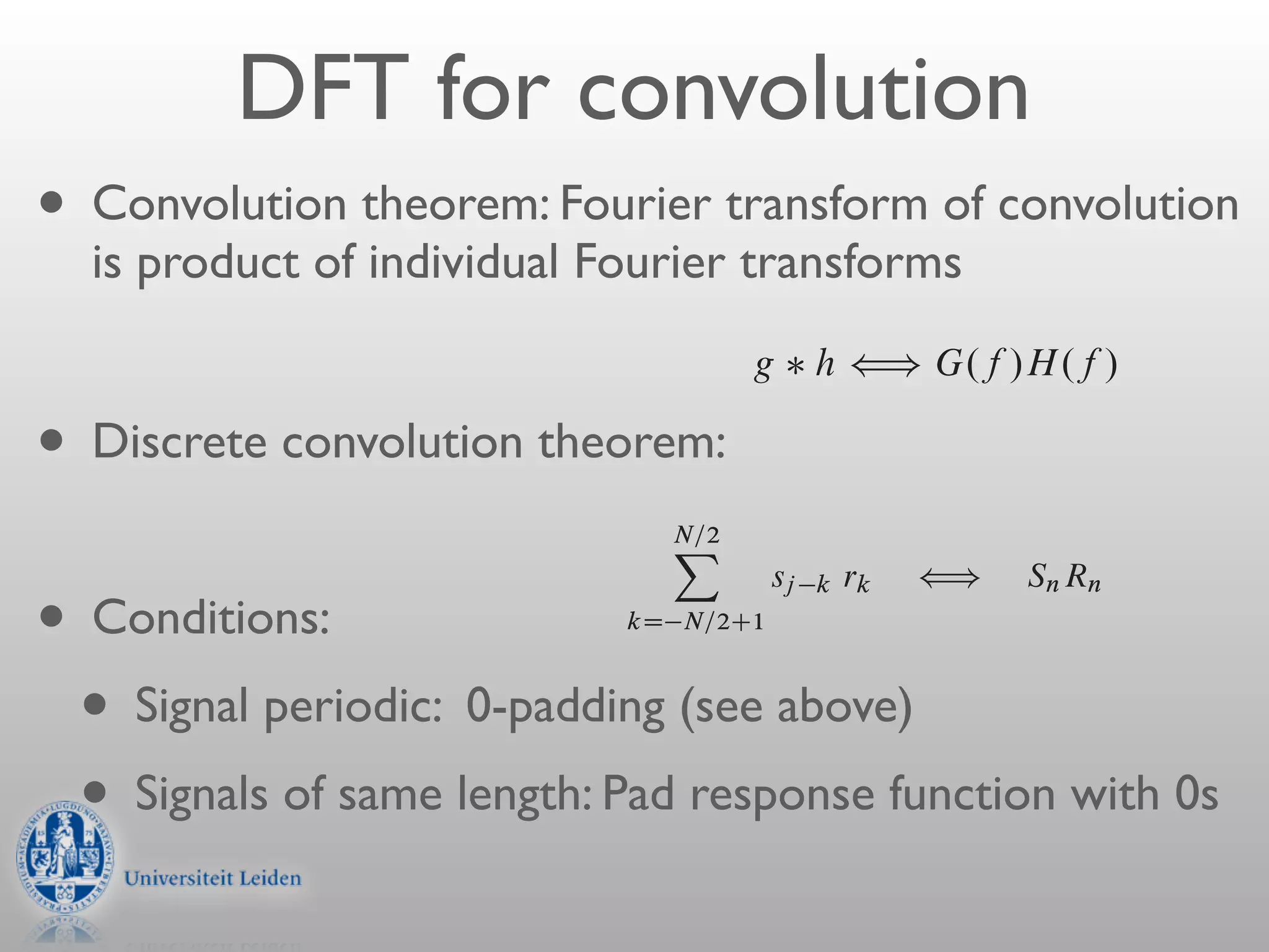
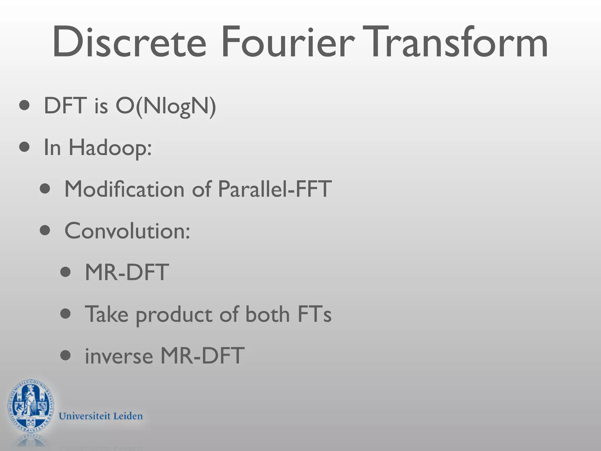
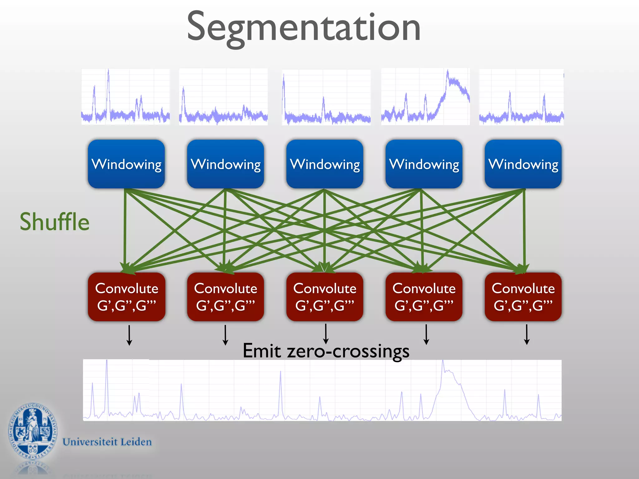
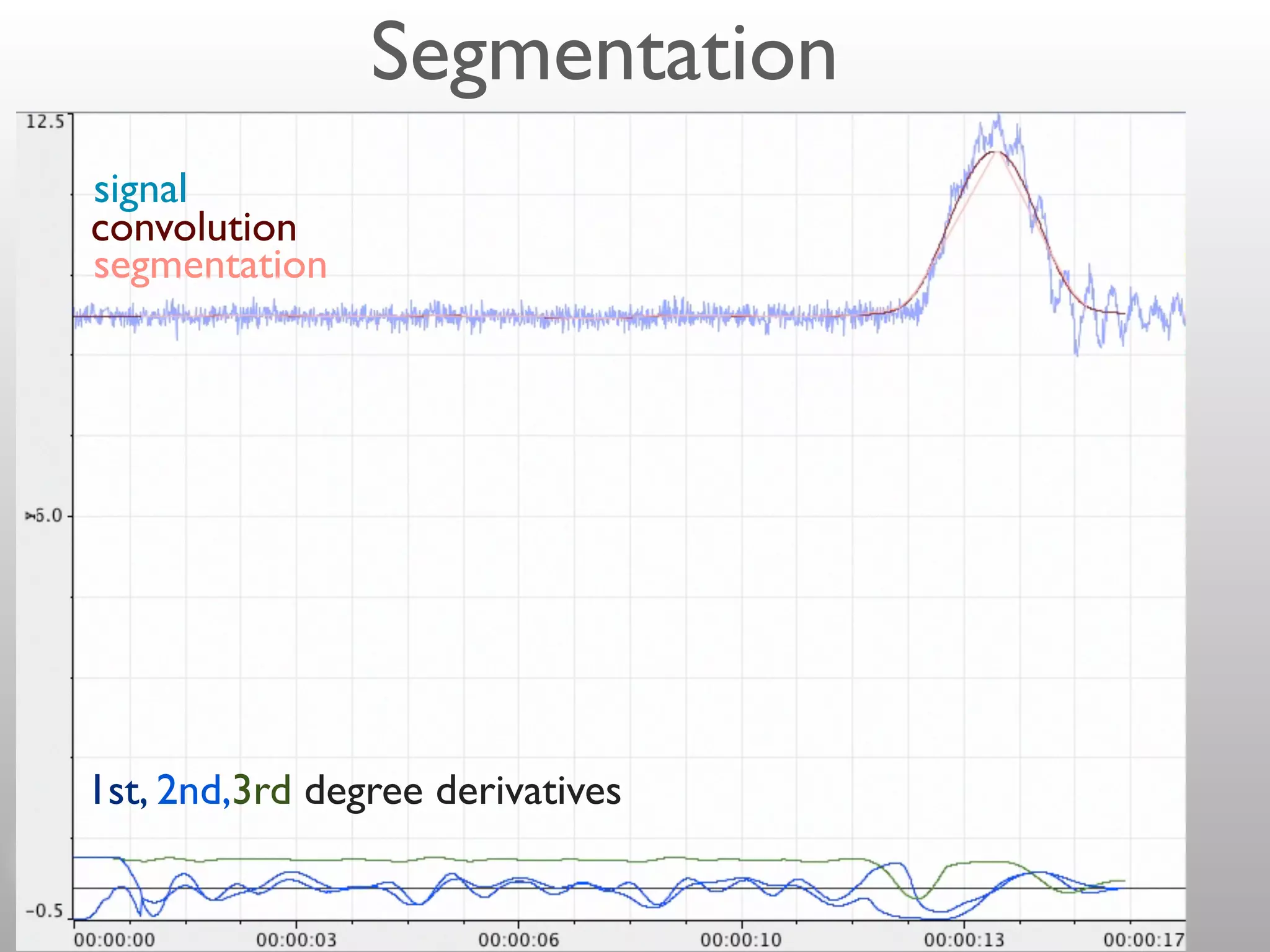
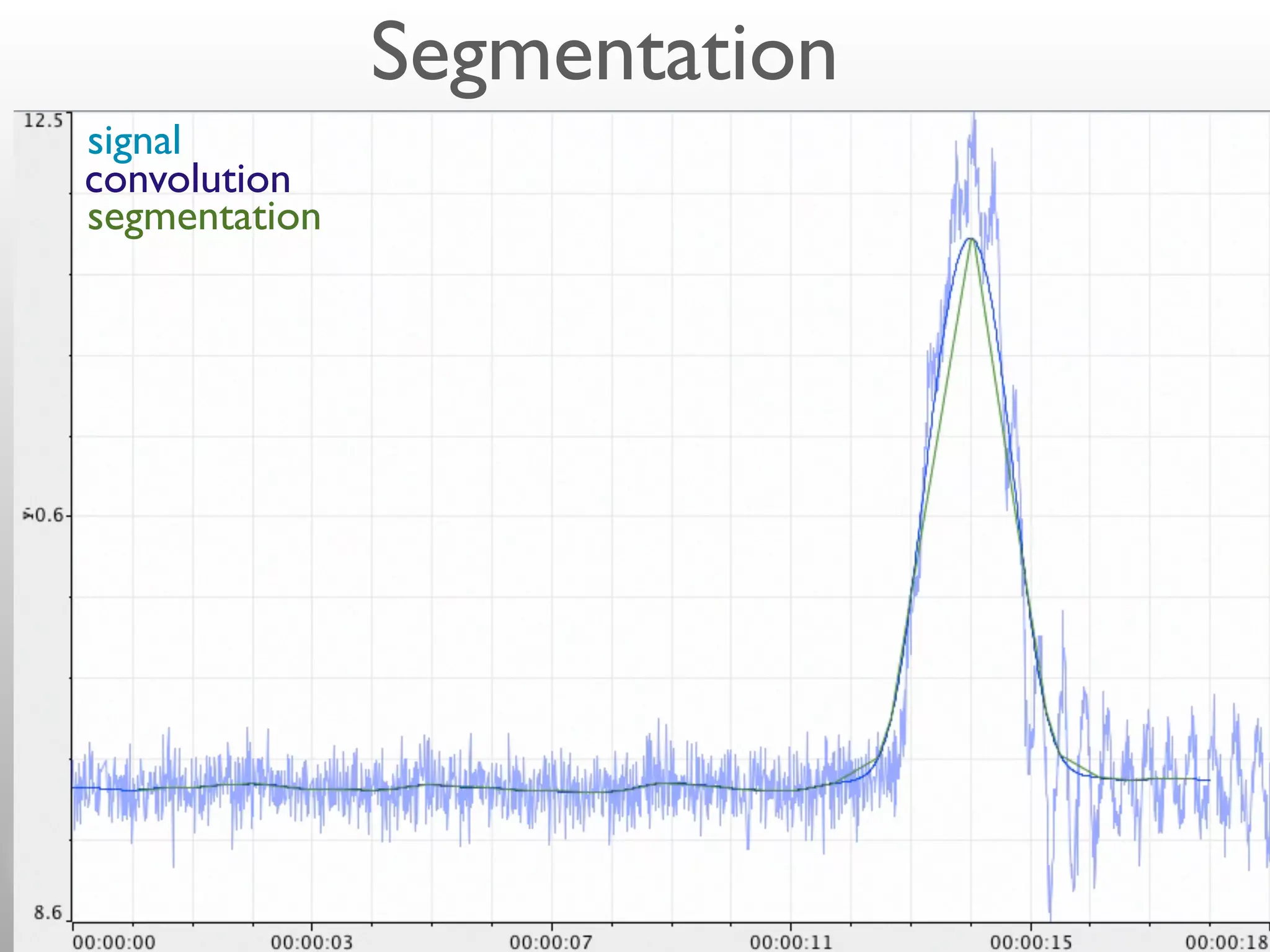
2 if0 t
                      h.t / e               ” H.f                 f /              frequency shiftin
                Figure 13.1.2. Convolution of discretely sampled functions. Note how the response function fo
                                                                     0

                            Convolution
                times is wrapped around and stored at the extreme right end of the array rk .
             With two functions h.t / and g.t /, and their corresponding
        H.f / and G.f /, we can form two combinations of special intere
•   Amount of Example: Abetween g functions 1asbyall other rk ’s equal
        of the two functions, denoted 2 h, is r0 D and
                    overlap response function with defined they are
    translatedjust the identity filter. Convolution Zis1signal with this response functio
              is                                      of a
              identically the signal. Another example the response function with r14 D
                                                hÁ
              all other rk ’s equal to zero.gThis produces convolved output / d is the inpu
                                                             g. /h.t        that
                                                       1
             multiplied by 1:5 and delayed by 14 sample intervals.

• In
                  Evidently, we have just described in words the following definition of
       practice: discrete a(sampled) theof finitedomain M : that g h D
        Note convolution witha function in signal s,duration and
             that g h is response function time short response
         that the function g            h is one member of a simple transform pair,
    function r (kernel)
                                                                  M=2
                                                                   X
                           g     h ” G.f /H.f /
                                      .r s/j Á                          convolution theorem
                                                                          sj k rk
                                                              kD M=2C1
         In other words, the Fourier transform of the convolution is just
         individual Fourier transforms.is nonzero only in some range M=2 < k Ä
              If a discrete response function
              The correlation of two functions, denoted Corr.g; h/, is defi
              where M is a sufficiently large even integer, then the response function is
              finite impulse response (FIR), and its duration is M . (Notice that we are defi
                                                        Z 1
              as the number of nonzero values of rk ; these values span a time interval of
                                       Corr.g; circumstances the C t /h. / d is the
              sampling times.) In most practicalh/ Á           g. case of finite M
                interest, either because the response really has1finite duration, or because we
                                                                a
2 if0 t
                        h.t / e               ” H.f                 f /              frequency shiftin
                  Figure 13.1.2. Convolution of discretely sampled functions. Note how the response function fo
                                                                       0

                              Convolution
                  times is wrapped around and stored at the extreme right end of the array rk .
               With two functions h.t / and g.t /, and their corresponding
          H.f / and G.f /, we can form two combinations of special intere
  •   Amount of Example: Abetween g functions 1asbyall other rk ’s equal
          of the two functions, denoted 2 h, is r0 D and
                      overlap response function with defined they are
      translatedjust the identity filter. Convolution Zis1signal with this response functio
                is                                      of a
                identically the signal. Another example the response function with r14 D
                                                  hÁ
                all other rk ’s equal to zero.gThis produces convolved output / d is the inpu
                                                               g. /h.t        that
                                                         1
               multiplied by 1:5 and delayed by 14 sample intervals.

  • In
                    Evidently, we have just described in words the following definition of
         practice: discrete a(sampled) theof finitedomain M : that g h D
          Note convolution witha function in signal s,duration and
               that g h is response function time short response
           that the function g            h is one member of a simple transform pair,
      function r (kernel)
                                                                    M=2
                                                                     X
                             g     h ” G.f /H.f /
                                        .r s/j Á                          convolution theorem
                                                                            sj k rk
                                                                kD M=2C1
         In other words, the Fourier transform of the convolution is just
         individual Fourier transforms.
convolution If a discrete response function is nonzero only in some range M=2 < k Ä
              The correlation of two functions, denoted Corr.g; h/, is defi
              where M is a sufficiently large even integer, then the response function is
signal        finite impulse response (FIR), and its duration is M . (Notice that we are defi
                                                          Z 1
              as the number of nonzero values of rk ; these values span a time interval of
                                        Corr.g; circumstances the C t /h. / d is the
              sampling times.) In most practicalh/ Á            g. case of finite M
kernel        interest, either because the response really has1finite duration, or because we
                                                              a
Convolution
• Width of kernel defines smoothing strength
Convolution
 • Width of kernel defines smoothing strength
convolution 1
convolution 2
signal
kernel 1
kernel 2
Convolution
 • Width of kernel defines smoothing strength
convolution 1
convolution 2
signal
kernel 1
kernel 2

 • Quite fast (O(N*M)), not fast enough
Convolution
 • Width of kernel defines smoothing strength
convolution 1
convolution 2
signal
kernel 1
kernel 2

 • Quite fast (O(N*M)), not fast enough
Map


Reduce
Map


Reduce
Map     Map   Map   Map   Map


Reduce
Map      Map      Map      Map      Map


Reduce   Reduce   Reduce   Reduce   Reduce
Map      Map      Map      Map      Map


Reduce   Reduce   Reduce   Reduce   Reduce
Build     Build     Build     Build     Build
  Map       Map       Map       Map       Map
windows   windows   windows   windows   windows


Reduce    Reduce    Reduce    Reduce    Reduce
Build     Build     Build     Build     Build
  Map       Map       Map       Map       Map
windows   windows   windows   windows   windows


Reduce    Reduce    Reduce    Reduce    Reduce
Build     Build     Build     Build     Build
           Map       Map       Map       Map       Map
         windows   windows   windows   windows   windows


Shuffle

         Reduce    Reduce    Reduce    Reduce    Reduce
Build       Build       Build       Build       Build
           Map         Map         Map         Map         Map
         windows     windows     windows     windows     windows


Shuffle

          Reduce
         Convolute    Reduce
                     Convolute    Reduce
                                 Convolute    Reduce
                                             Convolute    Reduce
                                                         Convolute
i
    Convolution in Hadoop
                  “nr3” — 2007/5/1 — 20:53 — page 644 — #666


            644
• Wrap-around problem
                            Chapter 13. Fourier and Spectral Applications


                                         response function


                    m+                                                  m−


                                   sample of original function               m+

                   m−


                                          convolution

                  spoiled                  unspoiled                 spoiled
Convolution in Hadoop    spoiled
                                                    convolution

                                                     unspoiled                         spoiled


• Wrap-around problem
             Figure 13.1.3. The wraparound problem in convolving finite segments of a function. Not only must
             the response function wrap be viewed as cyclic, but so must the sampled original function. Therefore,
             a portion at each end of the original function is erroneously wrapped around by convolution with the


 • Ignore spoiled regions
             response function.


                                      response function

 • Mirror the sequence (works well in our case)
                  m+                                                        m−


 • Zero-padding
                                           original function                                 zero padding

                       m−                                                                                m+


                                  not spoiled because zero

                  m+                                                                                m−

                        unspoiled                                                                spoiled
                                                                                              but irrelevant
Convolution in Hadoop
• Data split problem: windowing
 • `Overlap-convolute’
Convolution in Hadoop
 • Data split problem: windowing
  • `Overlap-convolute’
Map
(window)
           timestamp1
                        timestamp2

                                     timestamp3
Convolution in Hadoop
 • Data split problem: windowing
  • `Overlap-convolute’
              Mapper1         Mapper2         Mapper3
Map
(window)       1        2 1     2       3 2    3
           timestamp1
                          timestamp2

                                          timestamp3
Convolution in Hadoop
  • Data split problem: windowing
   • `Overlap-convolute’
                 Mapper1         Mapper2         Mapper3
Map
(window)          1        2 1     2       3 2    3
              timestamp1
                             timestamp2
Reduce
(convolute)                                  timestamp3


              Emit only unpolluted data
Convolution in Hadoop
• Data split problem: windowing
 • `Convolute-add’
Convolution in Hadoop
  • Data split problem: windowing
   • `Convolute-add’
Map          0             0
(convolute             0                0
with 0-padding)                             0
                                    0
Convolution in Hadoop
  • Data split problem: windowing
   • `Convolute-add’
Map
(convolute
with 0-padding)

Reduce
(add)                 A       A+B      B     B+C      C

                  Add values in overlapping regions
Hint: Keep mappers alive

• Mappers will be killed if you spend too much
  time in a loop (e.g. during long convolutions)
• Do this in large loops:
 • for(loopcount%1000==0){context.progress();}
Even faster: Fourier Transform
• Converts signal from time domain to frequency domain
 • Stress sensor (time domain)
 •f

 • Fourier transform (frequency domain)
Discrete Fourier Transform
• Converts signal from time domain to frequency domain
 • Vibration sensor (time domain)


 • Fourier transform (frequency domain)
H.f / and G.f /, we can form two combinatio
                                       of the two functions, denoted g h, is defined
                DFT for convolution                               g hÁ
                                                                        Z 1
                                                                               g. /h
    • Convolution theorem: Note that gtransform of convolution
        i                  Fourier
                                        h is a function in the time domai
                                                                                   1


        is product of individualthat the 2007/5/1 — 20:53 one page 643 of a#665
                                 Fourier transforms— member — sim
i
                              “nr3” — function g h is

                                                      g   h ” G.f /H.f /               conv

    •   Discrete convolution13.1 Convolution and the Fourier transform FFTthe c
                             theorem:
                              In other words, Deconvolution Using the of
                                       individual Fourier transforms.
                                            The correlation of two functions, denoted
                                              N=2
                                              X
                                                     sj k rk ” Sn Rn Z 1
    • Conditions:                           kD N=2C1           Corr.g; h/ Á      g.
                                                                                       1

      • Signal periodic: 0-padding (see above) of t , which is call
                    Here Sn .n D 0; : : : ; N 1/ is the discrete Fourier transform of the valu
                             The correlation is a function
                    0; : : : ; N 1/, while Rn .n D 0; : : : ; N 1/ is the discrete Fourier t

      • Signals of same length: Pad response ” G.f /H .f /0s c
                             domain, and it turns out to be one member of t
                    the values rk .k D 0; : : : ; N 1/. These values of rk are the same as f
                                                    function with
                    k D N=2 C 1; : : : ; N=2, but in wraparound order, exactly as was desc
                    end of 12.2.      Corr.g; h/

                    13.1.1 Treatment of End Effects by Zero Paddingpai
                                 [More generally, the second member of the
Discrete Fourier Transform
• DFT is O(NlogN)
• In Hadoop:
  • Modification of Parallel-FFT
  • Convolution:
    • MR-DFT
    • Take product of both FTs
    • inverse MR-DFT
Segmentation


         Windowing     Windowing     Windowing     Windowing     Windowing


Shuffle

         Convolute     Convolute     Convolute     Convolute     Convolute
         G’,G’’,G’’’   G’,G’’,G’’’   G’,G’’,G’’’   G’,G’’,G’’’   G’,G’’,G’’’


                               Emit zero-crossings
Segmentation
signal
convolution
segmentation


1st, 2nd,3rd degree derivatives
Segmentation
signal
convolution
segmentation

Hadoop sensordata part2

  • 1.
    2 if0 t h.t / e ” H.f f / frequency shiftin Figure 13.1.2. Convolution of discretely sampled functions. Note how the response function fo 0 Convolution times is wrapped around and stored at the extreme right end of the array rk . With two functions h.t / and g.t /, and their corresponding H.f / and G.f /, we can form two combinations of special intere • Amount of Example: Abetween g functions 1asbyall other rk ’s equal of the two functions, denoted 2 h, is r0 D and overlap response function with defined they are translatedjust the identity filter. Convolution Zis1signal with this response functio is of a identically the signal. Another example the response function with r14 D hÁ all other rk ’s equal to zero.gThis produces convolved output / d is the inpu g. /h.t that 1 multiplied by 1:5 and delayed by 14 sample intervals. • In Evidently, we have just described in words the following definition of practice: discrete a(sampled) theof finitedomain M : that g h D Note convolution witha function in signal s,duration and that g h is response function time short response that the function g h is one member of a simple transform pair, function r (kernel) M=2 X g h ” G.f /H.f / .r s/j Á convolution theorem sj k rk kD M=2C1 In other words, the Fourier transform of the convolution is just individual Fourier transforms.is nonzero only in some range M=2 < k Ä If a discrete response function The correlation of two functions, denoted Corr.g; h/, is defi where M is a sufficiently large even integer, then the response function is finite impulse response (FIR), and its duration is M . (Notice that we are defi Z 1 as the number of nonzero values of rk ; these values span a time interval of Corr.g; circumstances the C t /h. / d is the sampling times.) In most practicalh/ Á g. case of finite M interest, either because the response really has1finite duration, or because we a
  • 2.
    2 if0 t h.t / e ” H.f f / frequency shiftin Figure 13.1.2. Convolution of discretely sampled functions. Note how the response function fo 0 Convolution times is wrapped around and stored at the extreme right end of the array rk . With two functions h.t / and g.t /, and their corresponding H.f / and G.f /, we can form two combinations of special intere • Amount of Example: Abetween g functions 1asbyall other rk ’s equal of the two functions, denoted 2 h, is r0 D and overlap response function with defined they are translatedjust the identity filter. Convolution Zis1signal with this response functio is of a identically the signal. Another example the response function with r14 D hÁ all other rk ’s equal to zero.gThis produces convolved output / d is the inpu g. /h.t that 1 multiplied by 1:5 and delayed by 14 sample intervals. • In Evidently, we have just described in words the following definition of practice: discrete a(sampled) theof finitedomain M : that g h D Note convolution witha function in signal s,duration and that g h is response function time short response that the function g h is one member of a simple transform pair, function r (kernel) M=2 X g h ” G.f /H.f / .r s/j Á convolution theorem sj k rk kD M=2C1 In other words, the Fourier transform of the convolution is just individual Fourier transforms. convolution If a discrete response function is nonzero only in some range M=2 < k Ä The correlation of two functions, denoted Corr.g; h/, is defi where M is a sufficiently large even integer, then the response function is signal finite impulse response (FIR), and its duration is M . (Notice that we are defi Z 1 as the number of nonzero values of rk ; these values span a time interval of Corr.g; circumstances the C t /h. / d is the sampling times.) In most practicalh/ Á g. case of finite M kernel interest, either because the response really has1finite duration, or because we a
  • 3.
    Convolution • Width ofkernel defines smoothing strength
  • 4.
    Convolution • Widthof kernel defines smoothing strength convolution 1 convolution 2 signal kernel 1 kernel 2
  • 5.
    Convolution • Widthof kernel defines smoothing strength convolution 1 convolution 2 signal kernel 1 kernel 2 • Quite fast (O(N*M)), not fast enough
  • 6.
    Convolution • Widthof kernel defines smoothing strength convolution 1 convolution 2 signal kernel 1 kernel 2 • Quite fast (O(N*M)), not fast enough
  • 7.
  • 8.
  • 9.
    Map Map Map Map Map Reduce
  • 10.
    Map Map Map Map Map Reduce Reduce Reduce Reduce Reduce
  • 11.
    Map Map Map Map Map Reduce Reduce Reduce Reduce Reduce
  • 12.
    Build Build Build Build Build Map Map Map Map Map windows windows windows windows windows Reduce Reduce Reduce Reduce Reduce
  • 13.
    Build Build Build Build Build Map Map Map Map Map windows windows windows windows windows Reduce Reduce Reduce Reduce Reduce
  • 14.
    Build Build Build Build Build Map Map Map Map Map windows windows windows windows windows Shuffle Reduce Reduce Reduce Reduce Reduce
  • 15.
    Build Build Build Build Build Map Map Map Map Map windows windows windows windows windows Shuffle Reduce Convolute Reduce Convolute Reduce Convolute Reduce Convolute Reduce Convolute
  • 16.
    Build Build Build Build Build Map Map Map Map Map windows windows windows windows windows Shuffle Reduce Convolute Reduce Convolute Reduce Convolute Reduce Convolute Reduce Convolute
  • 17.
    Build Build Build Build Build Map Map Map Map Map windows windows windows windows windows Shuffle Reduce Convolute Reduce Convolute Reduce Convolute Reduce Convolute Reduce Convolute
  • 18.
    i Convolution in Hadoop “nr3” — 2007/5/1 — 20:53 — page 644 — #666 644 • Wrap-around problem Chapter 13. Fourier and Spectral Applications response function m+ m− sample of original function m+ m− convolution spoiled unspoiled spoiled
  • 19.
    Convolution in Hadoop spoiled convolution unspoiled spoiled • Wrap-around problem Figure 13.1.3. The wraparound problem in convolving finite segments of a function. Not only must the response function wrap be viewed as cyclic, but so must the sampled original function. Therefore, a portion at each end of the original function is erroneously wrapped around by convolution with the • Ignore spoiled regions response function. response function • Mirror the sequence (works well in our case) m+ m− • Zero-padding original function zero padding m− m+ not spoiled because zero m+ m− unspoiled spoiled but irrelevant
  • 20.
    Convolution in Hadoop •Data split problem: windowing • `Overlap-convolute’
  • 21.
    Convolution in Hadoop • Data split problem: windowing • `Overlap-convolute’ Map (window) timestamp1 timestamp2 timestamp3
  • 22.
    Convolution in Hadoop • Data split problem: windowing • `Overlap-convolute’ Mapper1 Mapper2 Mapper3 Map (window) 1 2 1 2 3 2 3 timestamp1 timestamp2 timestamp3
  • 23.
    Convolution in Hadoop • Data split problem: windowing • `Overlap-convolute’ Mapper1 Mapper2 Mapper3 Map (window) 1 2 1 2 3 2 3 timestamp1 timestamp2 Reduce (convolute) timestamp3
  • 24.
    Convolution in Hadoop • Data split problem: windowing • `Overlap-convolute’ Mapper1 Mapper2 Mapper3 Map (window) 1 2 1 2 3 2 3 timestamp1 timestamp2 Reduce (convolute) timestamp3 Emit only unpolluted data
  • 25.
    Convolution in Hadoop •Data split problem: windowing • `Convolute-add’
  • 26.
    Convolution in Hadoop • Data split problem: windowing • `Convolute-add’ Map 0 0 (convolute 0 0 with 0-padding) 0 0
  • 27.
    Convolution in Hadoop • Data split problem: windowing • `Convolute-add’ Map (convolute with 0-padding) Reduce (add) A A+B B B+C C Add values in overlapping regions
  • 28.
    Hint: Keep mappersalive • Mappers will be killed if you spend too much time in a loop (e.g. during long convolutions) • Do this in large loops: • for(loopcount%1000==0){context.progress();}
  • 29.
    Even faster: FourierTransform • Converts signal from time domain to frequency domain • Stress sensor (time domain) •f • Fourier transform (frequency domain)
  • 30.
    Discrete Fourier Transform •Converts signal from time domain to frequency domain • Vibration sensor (time domain) • Fourier transform (frequency domain)
  • 31.
    H.f / andG.f /, we can form two combinatio of the two functions, denoted g h, is defined DFT for convolution g hÁ Z 1 g. /h • Convolution theorem: Note that gtransform of convolution i Fourier h is a function in the time domai 1 is product of individualthat the 2007/5/1 — 20:53 one page 643 of a#665 Fourier transforms— member — sim i “nr3” — function g h is g h ” G.f /H.f / conv • Discrete convolution13.1 Convolution and the Fourier transform FFTthe c theorem: In other words, Deconvolution Using the of individual Fourier transforms. The correlation of two functions, denoted N=2 X sj k rk ” Sn Rn Z 1 • Conditions: kD N=2C1 Corr.g; h/ Á g. 1 • Signal periodic: 0-padding (see above) of t , which is call Here Sn .n D 0; : : : ; N 1/ is the discrete Fourier transform of the valu The correlation is a function 0; : : : ; N 1/, while Rn .n D 0; : : : ; N 1/ is the discrete Fourier t • Signals of same length: Pad response ” G.f /H .f /0s c domain, and it turns out to be one member of t the values rk .k D 0; : : : ; N 1/. These values of rk are the same as f function with k D N=2 C 1; : : : ; N=2, but in wraparound order, exactly as was desc end of 12.2. Corr.g; h/ 13.1.1 Treatment of End Effects by Zero Paddingpai [More generally, the second member of the
  • 32.
    Discrete Fourier Transform •DFT is O(NlogN) • In Hadoop: • Modification of Parallel-FFT • Convolution: • MR-DFT • Take product of both FTs • inverse MR-DFT
  • 33.
    Segmentation Windowing Windowing Windowing Windowing Windowing Shuffle Convolute Convolute Convolute Convolute Convolute G’,G’’,G’’’ G’,G’’,G’’’ G’,G’’,G’’’ G’,G’’,G’’’ G’,G’’,G’’’ Emit zero-crossings
  • 34.
  • 35.