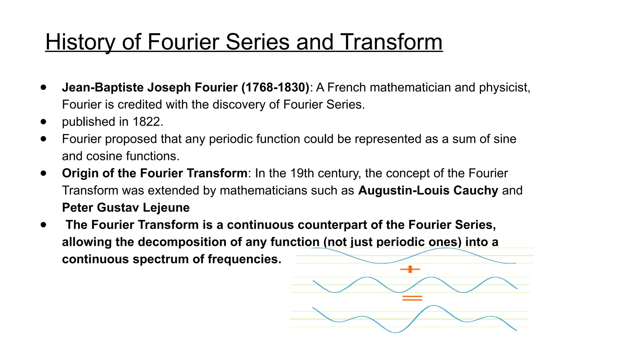
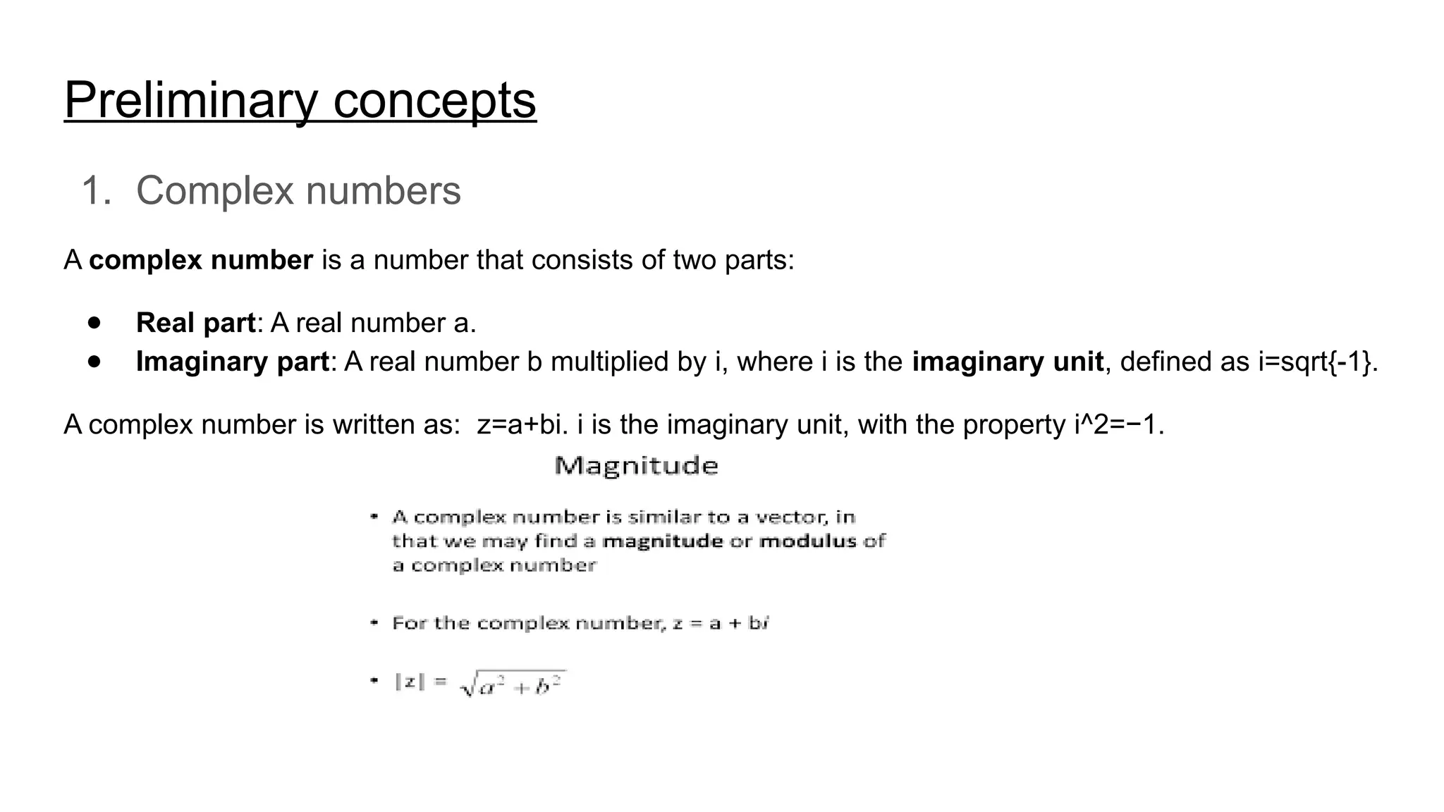
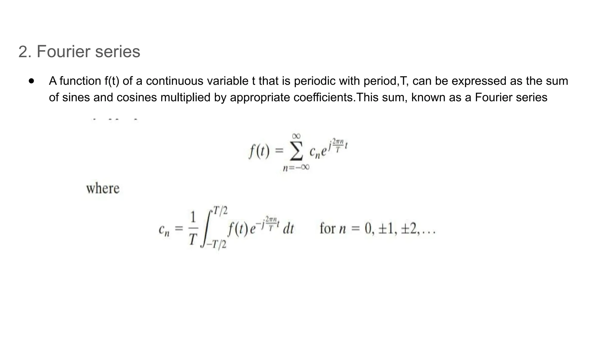
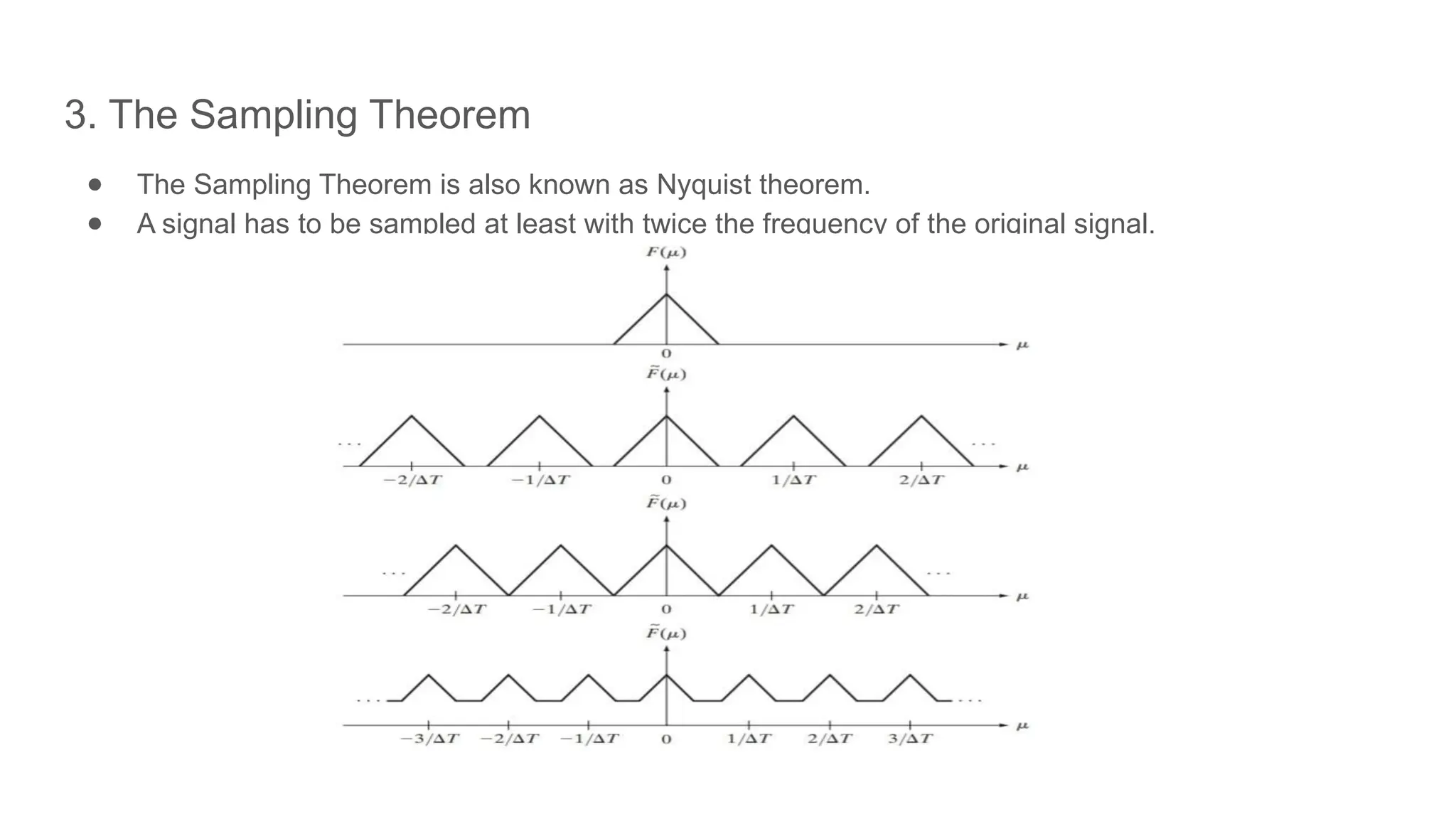
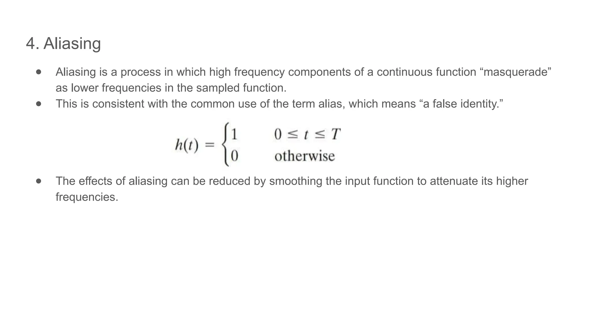
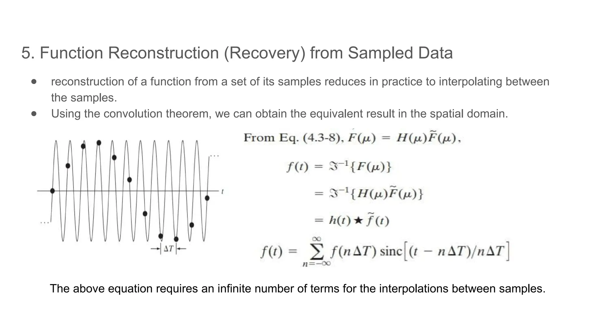
FILTERING IN THE
FREQUENCY DOMAIN
Name: Deepraj G Kamble
USN: 2GP21EC013
Sem: 7th
History of Fourier Series and Transform
● Jean-Baptiste Joseph Fourier (1768-1830): A French mathematician and physicist,
Fourier is credited with the discovery of Fourier Series.
● published in 1822.
● Fourier proposed that any periodic function could be represented as a sum of sine
and cosine functions.
● Origin of the Fourier Transform: In the 19th century, the concept of the Fourier
Transform was extended by mathematicians such as Augustin-Louis Cauchy and
Peter Gustav Lejeune
● The Fourier Transform is a continuous counterpart of the Fourier Series,
allowing the decomposition of any function (not just periodic ones) into a
continuous spectrum of frequencies.
Preliminary concepts
1. Complex numbers
A complex number is a number that consists of two parts:
● Real part: A real number a.
● Imaginary part: A real number b multiplied by i, where i is the imaginary unit, defined as i=sqrt{-1}.
A complex number is written as: z=a+bi. i is the imaginary unit, with the property i^2=−1.
2. Fourier series
● A function f(t) of a continuous variable t that is periodic with period,T, can be expressed as the sum
of sines and cosines multiplied by appropriate coefficients.This sum, known as a Fourier series
3. Impulses and Their Sifting Property
● A unit impulse of a continuous variable t located at denoted is defined as
● An impulse has the so called sifting property with respect to integration
4. The Fourier Transform of Functions of One Continuous Variable
● The Fourier transform of a continuous function f(t) of a continuous variable t, is defined by the
equation:
● we can obtain f(t) back using the inverse Fourier transform:
5. Convolution
● convolution of two functions involves flipping (rotating by 180°) one function about its origin and
sliding it past the other.
● convolution of two continuous functions, f(t) and h(t), of one continuous variable t, is denoted as:
● The Fourier transform of this equation is,
Sampling and the Fourier Transform of Sampled Functions
1. Sampling
● Continuous functions have to be converted into a sequence of discrete values before they can be
processed in a computer. This is accomplished by using sampling and quantization.
● One way to model sampling is to multiply f(t) by a
sampling function equal to a train of impulses units
apart.
2. The Fourier Transform of Sampled Functions
● Let F(u) denote the Fourier transform of a continuous function f(t).
● The corresponding sampled function, is the product of f~(t) and an impulse train.
● The Fourier transform of the product of two functions in the spatial domain is the convolution of the
transforms of the two functions in the frequency domain.
● The Fourier transform F~(u), of the sampled function f~(t) is:
3. The Sampling Theorem
● The Sampling Theorem is also known as Nyquist theorem.
● A signal has to be sampled at least with twice the frequency of the original signal.
4. Aliasing
● Aliasing is a process in which high frequency components of a continuous function “masquerade”
as lower frequencies in the sampled function.
● This is consistent with the common use of the term alias, which means “a false identity.”
● The effects of aliasing can be reduced by smoothing the input function to attenuate its higher
frequencies.
5. Function Reconstruction (Recovery) from Sampled Data
● reconstruction of a function from a set of its samples reduces in practice to interpolating between
the samples.
● Using the convolution theorem, we can obtain the equivalent result in the spatial domain.
The above equation requires an infinite number of terms for the interpolations between samples.
THANK YOU

Untitled presentation.pptx deepraj Kamble

  • 1.
    FILTERING IN THE FREQUENCYDOMAIN Name: Deepraj G Kamble USN: 2GP21EC013 Sem: 7th
  • 2.
    History of FourierSeries and Transform ● Jean-Baptiste Joseph Fourier (1768-1830): A French mathematician and physicist, Fourier is credited with the discovery of Fourier Series. ● published in 1822. ● Fourier proposed that any periodic function could be represented as a sum of sine and cosine functions. ● Origin of the Fourier Transform: In the 19th century, the concept of the Fourier Transform was extended by mathematicians such as Augustin-Louis Cauchy and Peter Gustav Lejeune ● The Fourier Transform is a continuous counterpart of the Fourier Series, allowing the decomposition of any function (not just periodic ones) into a continuous spectrum of frequencies.
  • 3.
    Preliminary concepts 1. Complexnumbers A complex number is a number that consists of two parts: ● Real part: A real number a. ● Imaginary part: A real number b multiplied by i, where i is the imaginary unit, defined as i=sqrt{-1}. A complex number is written as: z=a+bi. i is the imaginary unit, with the property i^2=−1.
  • 4.
    2. Fourier series ●A function f(t) of a continuous variable t that is periodic with period,T, can be expressed as the sum of sines and cosines multiplied by appropriate coefficients.This sum, known as a Fourier series
  • 5.
    3. Impulses andTheir Sifting Property ● A unit impulse of a continuous variable t located at denoted is defined as ● An impulse has the so called sifting property with respect to integration
  • 6.
    4. The FourierTransform of Functions of One Continuous Variable ● The Fourier transform of a continuous function f(t) of a continuous variable t, is defined by the equation: ● we can obtain f(t) back using the inverse Fourier transform:
  • 7.
    5. Convolution ● convolutionof two functions involves flipping (rotating by 180°) one function about its origin and sliding it past the other. ● convolution of two continuous functions, f(t) and h(t), of one continuous variable t, is denoted as: ● The Fourier transform of this equation is,
  • 8.
    Sampling and theFourier Transform of Sampled Functions 1. Sampling ● Continuous functions have to be converted into a sequence of discrete values before they can be processed in a computer. This is accomplished by using sampling and quantization. ● One way to model sampling is to multiply f(t) by a sampling function equal to a train of impulses units apart.
  • 9.
    2. The FourierTransform of Sampled Functions ● Let F(u) denote the Fourier transform of a continuous function f(t). ● The corresponding sampled function, is the product of f~(t) and an impulse train. ● The Fourier transform of the product of two functions in the spatial domain is the convolution of the transforms of the two functions in the frequency domain. ● The Fourier transform F~(u), of the sampled function f~(t) is:
  • 10.
    3. The SamplingTheorem ● The Sampling Theorem is also known as Nyquist theorem. ● A signal has to be sampled at least with twice the frequency of the original signal.
  • 11.
    4. Aliasing ● Aliasingis a process in which high frequency components of a continuous function “masquerade” as lower frequencies in the sampled function. ● This is consistent with the common use of the term alias, which means “a false identity.” ● The effects of aliasing can be reduced by smoothing the input function to attenuate its higher frequencies.
  • 12.
    5. Function Reconstruction(Recovery) from Sampled Data ● reconstruction of a function from a set of its samples reduces in practice to interpolating between the samples. ● Using the convolution theorem, we can obtain the equivalent result in the spatial domain. The above equation requires an infinite number of terms for the interpolations between samples.
  • 13.