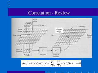
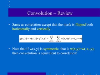
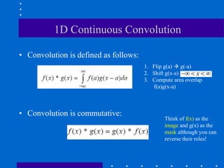
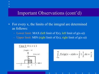
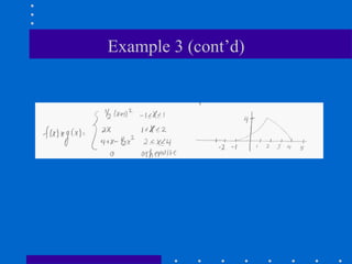
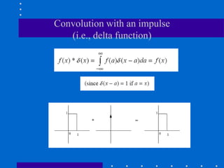
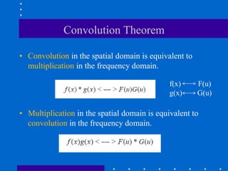
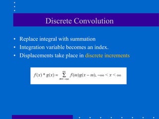
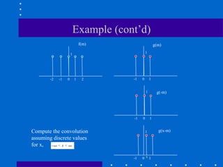
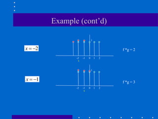
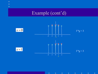
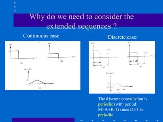
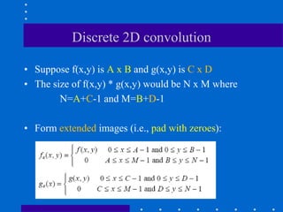
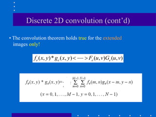
This document discusses convolution and correlation operations. It defines convolution as flipping a mask both horizontally and vertically before taking the weighted sum, while correlation does not include flipping. Convolution and correlation are equivalent if the mask is symmetric. The document also covers 1D and 2D continuous and discrete convolution, and explains how convolution in the spatial domain is equivalent to multiplication in the frequency domain via the Convolution Theorem.

1. Convolution
CS474/674 – Prof. Bebis
Section 3.4, 4.2

2. Correlation - Review
Output
Image
/2 /2
/2 /2
( , ) ( , ) ( , ) ( , ) ( , )
K K
s K t K
g x y w x y f x y w s t f x s y t
 
    
 
K x K

3. Convolution – Review
• Same as correlation except that the mask is flipped both
horizontally and vertically.
• Note that if w(x,y) is symmetric, that is w(x,y)=w(-x,-y),
then convolution is equivalent to correlation!
/2 /2
/2 /2
( , ) ( , ) ( , ) ( , ) ( , )
K K
s K t K
g x y w x y f x y w s t f x s y t
 
    
 

4. 1D Continuous Convolution
• Convolution is defined as follows:
• Convolution is commutative:
Think of f(x) as the
image and g(x) as the
mask although you can
reverse their roles!
1. Flip g(a)  g(-a)
2. Shift g(x-a)
3. Compute area overlap
f(a)g(x-a)
x
  

5. Example 1

6. Example 2
• Compute the convolution of the following two
functions:

7. Example 2 (cont’d)
x-1

8. Example 2 (cont’d)
Step 3: Compute the integral for x
  

9. Example 2 (cont’d)

10. Important Observations
• The extent of f(x) * g(x) is equal to the extent of f(x)
plus the extent of g(x)
extent = 1 extent = 1
extent = 2

11. Important Observations (cont’d)
• For every x, the limits of the integral are determined
as follows:
– Lower limit: MAX (left limit of f(x), left limit of g(x-a))
– Upper limit: MIN (right limit of f(x), right limit of g(x-a))

12. Example 3
α α
width = 2 width = 3

13. Example 3 (cont’d)

14. Example 3 (cont’d)

15. Convolution with an impulse
(i.e., delta function)

16. Convolution with an “train” of impulses
=

17. Convolution Theorem
• Convolution in the spatial domain is equivalent to
multiplication in the frequency domain.
• Multiplication in the spatial domain is equivalent to
convolution in the frequency domain.
f(x) F(u)
g(x) G(u)

18. Efficient computation of (f * g)
• 1. Compute and
• 2. Multiply them:
• 3. Compute the inverse FT:
We will later analyze computational complexity!
(i.e., element-wise
complex multiplication)

19. Discrete Convolution
• Replace integral with summation
• Integration variable becomes an index.
• Displacements take place in discrete increments

20. Example
5 samples 3 samples
f(m) g(m)
-1 0 1
-2 -1 0 1 2
1 1
*

21. Example (cont’d)
f(m) g(m)
-1 0 1
-2 -1 0 1 2
1 1
-1 0 1
1
-1 0 1
1
g(-m)
g(x-m)
x
Compute the convolution
assuming discrete values
for x,

22. Example (cont’d)
-4 -3 -2 -1 0 1 2
1
x
4 4
x or x
   
-3 -2 -1 0 1 2
1
x
3
x  
f *g = 0
f *g = 1
no overlap
Note that I show some
red samples “taller” for clarity!

23. Example (cont’d)
-2 -1 0 1 2
1
x
2
x  
1
x  
f *g = 2
f *g = 3
-2 -1 0 1 2
1
x

24. Example (cont’d)
0
x 
1
x 
f *g = 3
f *g = 3
-2 -1 0 1 2
1
x
-2 -1 0 1 2
1
x

25. Example (cont’d)
2
x 
3
x 
f *g = 2
f *g = 1
-2 -1 0 1 2 3 4
1
x
-2 -1 0 1 2 3
1
x
4
x  f *g = 0
no overlap

26. Example
5 samples 3 samples
f(m) g(m)
-1 0 1
1 1
* =
7 samples
-3 -2 -1 0 1 2 3
2
1
-2 -1 0 1 2
length of f*g = length of f + length of g - 1
3

27. Convolution Theorem in Discrete Case
• Input sequences:
• Length of f*g sequence is: M=A+B-1
• Extended input sequences: make them length M by
padding with zeroes:

28. Convolution Theorem in Discrete Case
(cont’d)
• When dealing with discrete convolution, the
convolution theorem holds true for the extended
sequences only!
Note: in general, we can form fe(x) and ge(x) using:
element-wise
complex multiplication

29. Why do we need to consider the
extended sequences ?
Continuous case Discrete case
The discrete convolution is
periodic (with period
M=A+B-1) since DFT is
periodic

30. Why do we need to consider the
extended sequences ? (cont’d)
If M<A+B-1, the periods move
closer to each other (overlap)
If M>A+B-1, the periods move
away from each other (no overlap)
Optimum:
M=A+B-1

31. 2D Convolution
• Definition
• 2D convolution theorem element-wise
complex multiplication

32. Discrete 2D convolution
• Suppose f(x,y) is A x B and g(x,y) is C x D
• The size of f(x,y) * g(x,y) would be N x M where
N=A+C-1 and M=B+D-1
• Form extended images (i.e., pad with zeroes):

33. Discrete 2D convolution (cont’d)
• The convolution theorem holds true for the extended
images only!
( , )* ( , ) ( , ) ( , )
e e e e
f x y g x y F u v G u v
  

34. Example