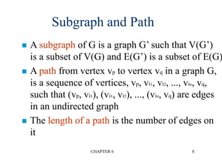
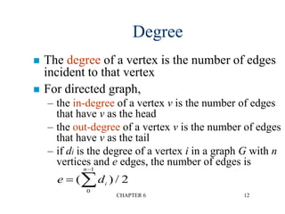
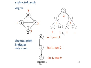
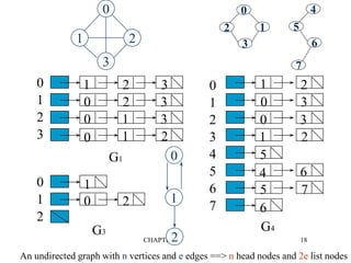
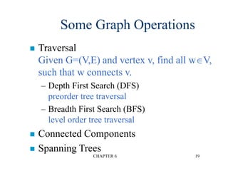
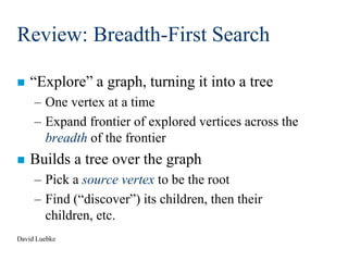
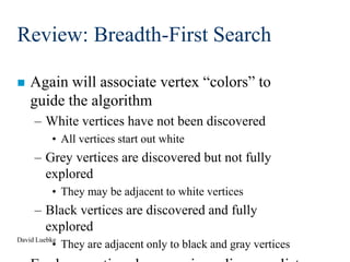
The document discusses graphs and graph algorithms. It defines graphs and their components such as vertices, edges, directed/undirected graphs. It provides examples of graphs and discusses graph representations using adjacency matrices and adjacency lists. It also describes common graph operations like traversal algorithms (depth-first search and breadth-first search), finding connected components, and spanning trees.

1. CHAPTER 6 1
CHAPTER 6
GRAPHS
All the programs in this file are selected from
Ellis Horowitz, Sartaj Sahni, and Susan Anderson-Freed
“Fundamentals of Data Structures in C”,
Computer Science Press, 1992.

2. CHAPTER 6 2
Definition
 A graph G consists of two sets
– a finite, nonempty set of vertices V(G)
– a finite, possible empty set of edges E(G)
– G(V,E) represents a graph
 An undirected graph is one in which the pair of
vertices in a edge is unordered, (v0, v1) = (v1,v0)
 A directed graph is one in which each edge is a
directed pair of vertices, <v0, v1> != <v1,v0>
tail head

3. CHAPTER 6 3
Examples for Graph
0
1 2
3
0
1
2
0
1 2
3 4 5 6
G1
G2
G3
V(G1)={0,1,2,3} E(G1)={(0,1),(0,2),(0,3),(1,2),(1,3),(2,3)}
V(G2)={0,1,2,3,4,5,6} E(G2)={(0,1),(0,2),(1,3),(1,4),(2,5),(2,6)}
V(G3)={0,1,2} E(G3)={<0,1>,<1,0>,<1,2>}
complete undirected graph: n(n-1)/2 edges
complete directed graph: n(n-1) edges
complete graph incomplete graph

4. CHAPTER 6 4
Complete Graph
 A complete graph is a graph that has the
maximum number of edges
– for undirected graph with n vertices, the maximum
number of edges is n(n-1)/2
– for directed graph with n vertices, the maximum
number of edges is n(n-1)
– example: G1 is a complete graph

5. CHAPTER 6 5

6. CHAPTER 6 6
Adjacent and Incident
 If (v0, v1) is an edge in an undirected graph,
– v0 and v1 are adjacent
– The edge (v0, v1) is incident on vertices v0 and v1
 If <v0, v1> is an edge in a directed graph
– v0 is adjacent to v1, and v1 is adjacent from v0
– The edge <v0, v1> is incident on v0 and v1

7. CHAPTER 6 7
0 2
1
(a)
2
1
0
3
(b)
*Figure 6.3:Example of a graph with feedback loops and a
multigraph (p.260)
self edge multigraph:
multiple occurrences
of the same edge
Figure 6.3

8. CHAPTER 6 8
 A subgraph of G is a graph G’ such that V(G’)
is a subset of V(G) and E(G’) is a subset of E(G)
 A path from vertex vp to vertex vq in a graph G,
is a sequence of vertices, vp, vi1, vi2, ..., vin, vq,
such that (vp, vi1), (vi1, vi2), ..., (vin, vq) are edges
in an undirected graph
 The length of a path is the number of edges on
it
Subgraph and Path

9. CHAPTER 6 9
0 0
1 2 3
1 2 0
1 2
3
(i) (ii) (iii) (iv)
(a) Some of the subgraph of G1
0 0
1
0
1
2
0
1
2
(i) (ii) (iii) (iv)
(b) Some of the subgraph of G3
分開
單一
0
1 2
3
G1
0
1
2
G3
Figure 6.4: subgraphs of G1 and G3 (p.261)

10. CHAPTER 6 10
 A simple path is a path in which all vertices,
except possibly the first and the last, are distinct
 A cycle is a simple path in which the first and
the last vertices are the same
 In an undirected graph G, two vertices, v0 and v1,
are connected if there is a path in G from v0 to v1
 An undirected graph is connected if, for every
pair of distinct vertices vi, vj, there is a path
from vi to vj
Simple Path and Style

11. CHAPTER 6 11
0
1 2
3
0
1 2
3 4 5 6
G1
G2
connected
tree (acyclic graph)

12. CHAPTER 6 12
Degree
 The degree of a vertex is the number of edges
incident to that vertex
 For directed graph,
– the in-degree of a vertex v is the number of edges
that have v as the head
– the out-degree of a vertex v is the number of edges
that have v as the tail
– if di is the degree of a vertex i in a graph G with n
vertices and e edges, the number of edges is
e di
n


( ) /
0
1
2

13. CHAPTER 6 13
undirected graph
degree
0
1 2
3 4 5 6
G1 G2
3
2
3 3
1 1 1 1
directed graph
in-degree
out-degree
0
1
2
G3
in:1, out: 1
in: 1, out: 2
in: 1, out: 0
0
1 2
3
33
3

14. CHAPTER 6 14
Graph Representations
 Adjacency Matrix
 Adjacency List

15. CHAPTER 6 15
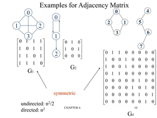
Adjacency Matrix
 Let G=(V,E) be a graph with n vertices.
 The adjacency matrix of G is a two-dimensional
n by n array, say adj_mat
 If the edge (vi, vj) is in E(G), adj_mat[i][j]=1
 If there is no such edge in E(G), adj_mat[i][j]=0
 The adjacency matrix for an undirected graph is
symmetric; the adjacency matrix for a digraph
need not be symmetric

16. CHAPTER 6 16
Examples for Adjacency Matrix
0
1
1
1
1
0
1
1
1
1
0
1
1
1
1
0












0
1
0
1
0
0
0
1
0










0
1
1
0
0
0
0
0
1
0
0
1
0
0
0
0
1
0
0
1
0
0
0
0
0
1
1
0
0
0
0
0
0
0
0
0
0
1
0
0
0
0
0
0
1
0
1
0
0
0
0
0
0
1
0
1
0
0
0
0
0
0
1
0


























G1
G2
G4
0
1 2
3
0
1
2
1
0
2
3
4
5
6
7
symmetric
undirected: n2/2
directed: n2

17. CHAPTER 6 17
Data Structures for Adjacency Lists
#define MAX_VERTICES 50
typedef struct node *node_pointer;
typedef struct node {
int vertex;
struct node *link;
};
node_pointer graph[MAX_VERTICES];
int n=0; /* vertices currently in use */
Each row in adjacency matrix is represented as an adjacency list.

18. CHAPTER 6 18
0
1
2
3
0
1
2
0
1
2
3
4
5
6
7
1 2 3
0 2 3
0 1 3
0 1 2
G1
1
0 2
G3
1 2
0 3
0 3
1 2
5
4 6
5 7
6
G4
0
1 2
3
0
1
2
1
0
2
3
4
5
6
7
An undirected graph with n vertices and e edges ==> n head nodes and 2e list nodes

19. CHAPTER 6 19
Some Graph Operations
 Traversal
Given G=(V,E) and vertex v, find all wV,
such that w connects v.
– Depth First Search (DFS)
preorder tree traversal
– Breadth First Search (BFS)
level order tree traversal
 Connected Components
 Spanning Trees

20. David Luebke
Review: Breadth-First Search
 “Explore” a graph, turning it into a tree
– One vertex at a time
– Expand frontier of explored vertices across the
breadth of the frontier
 Builds a tree over the graph
– Pick a source vertex to be the root
– Find (“discover”) its children, then their
children, etc.

21. David Luebke
Review: Breadth-First Search
 Again will associate vertex “colors” to
guide the algorithm
– White vertices have not been discovered
• All vertices start out white
– Grey vertices are discovered but not fully
explored
• They may be adjacent to white vertices
– Black vertices are discovered and fully
explored
• They are adjacent only to black and gray vertices

22. David Luebke
Depth-First Search
 Depth-first search is another strategy for
exploring a graph
– Explore “deeper” in the graph whenever
possible
– Edges are explored out of the most recently
discovered vertex v that still has unexplored
edges
– When all of v’s edges have been explored,
backtrack to the vertex from which v was
discovered