Applied mathematics for engineering and science students

1. 1
Chapter: Sequence and series
1.1 Definition and types of sequence
An infinite (real) sequence (more briefly, a sequence) is an unending succession of real numbers which
have a defined order consisting of a first number, a second number, a third number, and so on. Or
mathematically sequence of real numbers is a real-valued function 𝑓 defined on a set {𝑘, 𝑘 + 1, 𝑘 +
2, . . . } for some integer 𝑘.
Notation:
listing the terms in order as 𝑎1, 𝑎2, 𝑎3,. . . , 𝑎𝑛, . . . here 𝑎𝑛 is called the 𝑛𝑡ℎ
term of the sequence.
As a function of integers f(n) = an for n ≥ k (usually k=0 or 1) and n ∈ ℤ. Or as {an}n=k
∞
Note that: unless and otherwise specified the initial index k is the smallest integer which makes the
formula meaningful for all integers n ≥ k.
Types of sequence
Arithmetic sequence
Arithmetic Sequences: A sequence is arithmetic (arithmetic progression) if the difference between
two consecutive terms is constant.
Note:
1. An arithmetic sequence has the form 𝑎, 𝑎 + 𝑑, 𝑎 + 2𝑑, 𝑎 + 3𝑑, . . .
2. The constant d is called the common difference and it can be positive, negative or zero.
3. Each term of an arithmetic sequence is obtained from the preceding one by adding the common
difference d.
4. The formula for the 𝑛𝑡ℎ
term of an arithmetic sequence is 𝑎𝑛= 𝑎 + (𝑛 − 1)𝑑.
Example: The sequence of even numbers 2, 4, 6, 8, 10, ... is an arithmetic sequence in which the
common difference is d = 2.
Harmonic Sequence
Harmonic sequence (or harmonic progression) is a progression formed by taking the reciprocals of an
arithmetic progression.
The idea is, get every term in an arithmetic sequence and divide it to 1. The general form of a harmonic
sequence is;
1
𝑎
,
1
𝑎 + 𝑑
,
1
𝑎 + 2𝑑
,
1
𝑎 + 3𝑑
, . . . ,
1
𝑎 + 𝑘𝑑
, . . .
Examples: 1,
1
2
,
1
3
, . . . ,
1
𝑛
, . . .

2. 2
Geometric progression/sequences
A Geometric sequence is a sequence of numbers where each term in the sequence is found by
multiplying the previous term with an unchanging number called the common ratio.
The sequence 2, 6, 18, 54, . . . is a geometric sequence with a common ration 𝑟 = 3. Another
example of a geometric sequence is 10, 5, 2.5, 1.25, . . . with a common ratio 𝑟 =
1
2
.
Definition 1.1: A sequence  
n
a k
n


is said to be geometric with a common ratio a non-zero number 𝒓
if the terms of the sequence satisfy:
𝑎𝑛 = 𝑟𝑎𝑛−1, for all n.
Generally, it is preferable to express the term 𝑎𝑛 of a geometric sequence in function of 𝑟 and the initial
term 𝑎0, as in the formula:
𝑎𝑛 = 𝑎0𝑟𝑛
Recursively (Inductively) defined sequences:
Many mathematical patterns can be described using the idea of recursion.
Recursion is a process in which each step of a pattern is dependent on the step or steps that come before
it.
If the terms of a sequence are given in recursion form that is the beginning term or terms of a sequence
are given and then a recursive equation that defines the next terms of the sequence. Such a sequence is
called recursively defined sequence.
Examples of recursively defined sequences:
Geometric, arithmetic, population growth/decay
Fibonacci Sequences:
A special sequence generated recursively is the Fibonacci sequence, and characterized by the fact that
every number after the first two is the sum of the two preceding ones.
1, 1, 2, 3, 5, 8, 13, 21, 34, 55, 89, 144, 233, . . .
This can be defined by the recurrence relation:
𝑓1 = 1, 𝑓2 = 1, 𝑓
𝑛 = 𝑓𝑛−1 + 𝑓𝑛−2, 𝑛 ≥ 3
This sequence was first devised by the Italian Mathematician ( Leonardo of Pisa) to model rabbit
population. 𝑓
𝑛 represents the number of pairs of rabbits after n months, assuming that each month, a
pair of rabbit produces a new pair which becomes productive at age 2 months and no rabbit dies.

3. 3
1.2 Convergence properties of sequences
A fundamental question about a sequence {𝑎𝑛} concerns the behavior of its 𝑛𝑡ℎ
term 𝑎𝑛 as 𝑛 gets larger
and larger. For example, consider the sequence whose general term is given by:
𝑎𝑛 =
2𝑛−1
𝑛+1
, 𝑓𝑜𝑟 𝑛 ≥ 1.
Here the terms can be defined as 𝑎𝑛 =
2𝑛−1
𝑛+1
=
2𝑛+2−3
𝑛+1
=
2(𝑛+1)−3
𝑛+1
= 2 −
3
𝑛+1
It appears that
3
𝑛+1
closes to zero as 𝑛 increases without bound and consequently 𝑎𝑛 closes to 2.
Thus, we say that 2 1
lim 2
1
n
n
n


 

 

 
.
In general we say that lim( )
n
n
a L


if we can make n
a as close to L as we want for all sufficiently large n. In other words, the value of the
n
a ’𝑠 approaches 𝐿 as 𝑛 approaches infinity
The precise definition or formal definition of the above limits is defined as
 
lim n
n
a L


If for every positive number ε>0 there is an integer N such that
|an − L| < ε whenever n > N
In that case we say limit of the sequence exists and if limit exists and is finite we say that the sequence
is convergent.
For instance, in the above example one would expect
2 1
2
1
lim
n
n
n


 

 

 
2 1 3
2
1 1
n
n n


  
 
3
1
n

  
Thus, N should be some natural number larger than
3
𝜀
− 1. For example, If ε =
1
1000
, then we may
choose N to be any positive integer larger than 2999.
The Algebra of Convergent Sequences
Theorem 1.2 : If a sequence {𝑎𝑛} converges to A and {𝑏𝑛} converges to B, then the sequence
1. {𝑎𝑛 + 𝑏𝑛} converges to A+B
2. {𝑎𝑛 − 𝑏𝑛} converges to A-B
3. {𝑎𝑛𝑏𝑛} converges to AB
4. {𝑐𝑎𝑛} converges to cA for any constant c
5. {
𝑎𝑛
𝑏𝑛
} converges to
𝐴
𝐵
if B≠ 0
Definition 1.2 (Divergent sequence). For given sequences {𝑎𝑛} and {𝑏𝑛} , we have
a) lim(a )
n
n
  if and only if for each number 𝑅 > 0, there exists an integer 𝑁𝜖 ℕ such that 𝑎𝑛 >
𝑅 for all 𝑛 > 𝑁

4. 4
b) lim( )
n
n
b

  if and only if for each number 𝑅 < 0, there exists an integer 𝑁𝜖 ℕ such that
𝑏𝑛 < 𝑅 for all 𝑛 > 𝑁
We do not regard {𝑎𝑛} as a convergent sequence unless lim(a )
n
n
exists as a finite number, as require by
the definition. For instance, 2
lim( n )
n
   and lim( 4)
n
n

   .
We do not say that the sequence {−𝑛2} “converges to -∞” but rather that it “diverges to -∞” or “tends
to -∞.” To emphasize the distinction, we say that {𝑎𝑛} diverges to ∞ (respectively -∞) if lim(a )
n
n
 
(respectively -∞).
Definition 1.3 (Oscillatory sequence). A sequence that neither converges to a finite number nor
diverges to either ∞ or -∞ is said to oscillate or diverge by oscillation. An oscillating sequence with
finite amplitude is called a finitely oscillating sequence. An oscillating sequence with infinite amplitude
is called an infinitely oscillating sequence.
For instance, the sequences {(−1)n}, {1 + (−1)n}, {(−1)n
(1 +
1
n
)} oscillate finitely.
Remark: an unbounded sequence that does not diverge to ∞ or -∞ oscillates infinitely. For example,
the sequences {(−1)𝑛
𝑛2} and {(−𝑛)𝑛} are all unbounded and oscillate infinitely.
Techniques of evaluating limit of a convergent sequence
1. Continuous function representation
Proposition 1.3
Suppose {𝑎𝑛} be a sequence and 𝑓(𝑥) be a continuous function such that 𝑓(𝑛) = 𝑎𝑛 for all 𝑛 ≥ 𝑁 for
same integer N. then,
lim lim ( )
n
n n
a f x
 

Example:
For each of the following find the limit
a.
3
lim
n
n n

 
 
 
b.
2
1
lim
n
n n

 

 
 
Solution
a. Take 𝑓(𝑥) =
3𝑥
𝑥
, for 𝑥 ≥ 1
3 3
whichisinditerminate
lim lim
n x
n x
n x
 

 

Appling L’Hopital’s rule
 
 
3
3 ln(3)3
1
lim lim lim
x
x x
x x x
d
dx
d
x x
dx
  
 
 
   
 
 
 
Which implies
3
lim
n
n n

 
 
 
 
b. Take 𝑓(𝑥) = (1 −
2
𝑥
)
𝑥
for 𝑥 ≥ 1, then

5. 5
2
2 2
1 1
lim lim
n x
n x
e
n x

 
   
   
   
   
Proposition 1.4
a) lim , 0,
p
n
n for p

  
b)
1
lim 0, 0,
p
n
for p
n

 
c)
1
lim 1, 0,
n
n
a for a

 
d) If p(n) and q(n) are polynomials of n, then
0, if deg(p) deg(q),
( )
lim ,if deg(p) deg(q),
( )
,if deg(p) deg(q),where and aretheleadingcoefficientsof and .
n
p n
q n
a
a b p q
b


 

  


 

e)
( )
lim 0,foranypolynomial andanyrealnumber 1.
n
n
p n
p a
a

 
f)
( )
lim ,foranypolynomial andanyrealnumber 0.
ln( )
c
n
p n
p c
n

 
Theorem 1.5 (Continuous function theorem for sequences)
Let 𝑎𝑛 be a sequence converging to 𝑙 ∈ ℝ, and let 𝑓(𝑥) be a function that is defined on the range of 𝑎𝑛
and which is continuous at 𝑙. Then the sequence {𝑓(𝑎𝑛)} converges to 𝑓(𝑙).
Note that another way to state the continuous function theorem is that we can pass the limit through the
function when the above hypotheses are satisfied;
i.e., if (𝑎𝑛) →𝑙, if 𝑓(𝑎𝑛) is defined for each 𝑛 ∈ ℕ, and if 𝑓 is continuous at 𝑙, then
 
   
 
n
n
n
n
a
f
a
f




 lim
lim .
Example: Determine the convergence or divergence of
a.
 
2 1
sin
4
n
n

 

 
 
b.
 
  
















3
2
3
2
ln 2
2
n
n
n

6. 6
Solution:
a. Let 
n
b
 
2 1
sin
4
n
n

 

 
 
. Then 
n
b 
 n
n a
x
x
f
a
f ),
sin(
)
(
),
(
 
2 1
4
n
n

 

 
 
Now, 
n
a
 
2 1
4
n
n

 

 
 
1
2 2
4 4
n n

 
 
 
 
 
 
Since the harmonic sequence 0
1

n
and 2 2 ,4 4
 
  , we have
2
2 0
4 4 2
n

  


 
Thus, by continuous function theorem,
 
2 1
sin sin 1
4 2
n
n
 
 
  
 
   
 
 
b. Exercise
2. Rationalizing technique
Rationalizing makes use of the fact that
(𝑎 − 𝑏)(𝑎 + 𝑏) = 𝑎2
− 𝑏2
So, if either the first and/or the second term have a square root in them the rationalizing will eliminate
the root(s). This might help in evaluating the limit.
Example
Evaluate the limit of the sequence given by 𝑎𝑛 = √𝑛 + 1 − √𝑛, 𝑓𝑜𝑟 𝑛 ≥ 1
Solution:
lim lim( 1 ) (indeterminate)
n
n n
a n n
 
     
But when we rationalize as √𝑛 + 1 − √𝑛 = (√𝑛 + 1 − √𝑛)
√𝑛+1+√𝑛
√𝑛+1+√𝑛
=
1
√𝑛+1+√𝑛
, then
  1
lim 1 lim 0
1
n n
n n
n n
 
   
 
3.Theorem 1.6 (Squeeze theorem)
Given three sequences 𝑎𝑛, 𝑏𝑛, 𝑐𝑛, if 𝑎𝑛 ≤ 𝑏𝑛 ≤ 𝑐𝑛 for all n≥ 𝑁 and for some natural number N.
a) If  
lim lim( ) ,
n n
n n
a c L
 
  then also  
lim n
n
b L


b) If  
lim n
n
b

  then also lim( ) ,
n
n
c

 
c) If lim( ) ,
n
n
c

  then also  
lim n
n
b

 
proof (a):
Let 𝜀 > 0 be given. By the definition of convergence, there exist two numbers N1 and N2 such that
|𝑎𝑛 − 𝐿| < 𝜀 for all 𝑛 ≥ 𝑁1 and |𝑐𝑛 − 𝐿| < 𝜀 for all 𝑛 ≥ 𝑁2

7. 7
In particular since 𝑎𝑛 ≤ 𝑏𝑛 ≤ 𝑐𝑛 for all n≥ 𝑁, we have
𝐿 − 𝜀 < 𝑎𝑛 ≤ 𝑏𝑛 ≤ 𝑐𝑛 < 𝐿 + 𝜀 for 𝑛 ≥ 𝑁3 = Max{𝑁1, 𝑁2, 𝑁} ,
Showing that |𝑏𝑛 − 𝐿| < 𝜀 for all 𝑛 ≥ 𝑁3 as required.
The proof for b and c are left as exercise
Example 1: for any constant 𝑎 > 0 show that 0
!
lim
n
n
a
n

 

 
 
We can see that the sequence as recursively defined with the first term 𝑎1 = 𝑎, and each 𝑎𝑛 is obtained
by multiplying its predecessor by
𝑎
𝑛
.
Now, eventually, that is, for n large enough, we can obtain an integer 𝑛 so that
𝑎
𝑛
<
1
2
.
To be more precise, let N be the first integer for which
𝑎
𝑁
<
1
2
. Then for any 𝑘 > 0,
0 < 𝑎𝑛 =
𝑎𝑁+𝑘
(𝑁+𝑘)!
<
𝑎𝑁
𝑁!
1
2𝑘
Now the sequence on the right is a fixed number (
𝑎𝑁
𝑁!
) times a sequence(
1
2𝑘
) which tends to zero.
Thus, 0
!
lim
n
n
a
n

 

 
 
by the squeeze theorem
Example-2: For any positive integer p, show that lim 0
!
p
n
n
n

 .
4. Geometric sequence
A particularly common and useful sequence is a geometric sequence of the form 𝑎𝑛 = {𝑎0𝑟𝑛
}𝑛=0
∞
, for
various values of 𝑟 and 𝑎0 ≠ 0. Some are quite easy to understand:
If r = 1, the sequence will be constant sequence (i.e. 𝑎𝑛 = 𝑎0, 𝑓𝑜𝑟 𝑎𝑙𝑙 𝑛) and converges to 𝑎0 .
If r = -1, the sequence oscillates between 𝑎0 and −𝑎0 , thus diverges by oscillating.
If 0 < 𝑟 < 1, then the sequence converges to 0.
If −1 < 𝑟 < 0, then |𝑟𝑛| = |𝑟|𝑛
𝑎𝑛𝑑 0 < |𝑟| < 1, so the sequence converges to 0.
If 𝑟 > 1 𝑜𝑟 𝑟 < −1 , the terms 𝑎0𝑟𝑛
get larger positive or negative without limit, so the sequence
diverges.
In summary, 𝑎𝑛 = {𝑎0𝑟𝑛
} converges precisely when −1 < 𝑟 ≤ 1 in which case
0
0
a , 1
lim( ) 0, 1
, 1
n
n
if r
a r if r
if r

 

 


 


8. 8
5. Bounded and Monotonic sequences
Now we introduce some important terminology associated with sequences. A sequence {an} is said to
be:
 Bounded above if there exists an M ∈ R such that an≤ M for all n,
 Bounded below if there exists an m ∈ R such that an ≥ m for all n,
 Bounded if it is bounded both below and above,
 Monotonically increasing (or simply increasing) if an ≤ an+1for all n ,
 Monotonically decreasing (or simply decreasing) if an ≥ an+1for all n ,
 Monotonic if it is either increasing or decreasing.
Proposition 1.7. A convergent sequence is bounded.
Proof: Suppose {an} be convergent sequence and converges to 𝑎, then for 𝜀 = 1 there is an integer N
such that
|𝑎𝑛 − 𝑎| < 1 for all 𝑛 ≥ 𝑁
The triangle inequality |𝑎𝑛| ≤ |𝑎𝑛 − 𝑎| + |𝑎| < 1 + |𝑎| for all n≥ 𝑁
implies that for 𝑀 = 𝑀𝑎𝑥{|𝑎1|, |𝑎2|, . . . , |𝑎𝑁|, 1 + |𝑎|}
|𝑎𝑛| ≤ 𝑀 for all 𝑛 ≥ 1. Hence bounded
Thus, boundedness is a necessary condition for convergence but not sufficient condition, and every un-
bounded sequence diverges.
Theorem 1.8 : A monotone sequence of real numbers converges if and only if it is bounded.
If {an} is monotone increasing and bounded, then
   
:
lim n n
n
a Sup a n

  and
If {an} is monotone decreasing and bounded, then
   
:
lim n n
n
a Inf a n

 
Furthermore, if {an} is monotone increasing and unbounded, then
 
lim n
n
a

 
and if {an} is monotone decreasing and unbounded, then
 
lim n
n
a

 

9. 9
1.3 Definition of infinite series
Now we will investigate what may happen when we add all terms of a sequence together to form what
will be called an infinite series.
Definition: A series of real numbers is an expression of the form 𝑎1 + 𝑎2 + 𝑎3 + . . .
or more compactly as 

1
n
n
a where {𝑎𝑛} is a sequence of real numbers.
The number 𝑎𝑛 is called the nth
term of the series and the sequence  
n
s n

1
which is obtained by
adding the first n-terms of the series (i.e 𝑠𝑛 = 𝑎1 + 𝑎2 + 𝑎3 . . . + 𝑎𝑛 = 

n
i
i
a
1
) is called the 𝑛𝑡ℎ
partial sum of the series ∑ (𝑎𝑛)
∞
𝑛=1 .
Note that: it is customary to use initial index of a series any integer k which makes the formula of an
meaningful for all 𝑛 ≥ 𝑘.
1.4 Convergence and divergence, properties of series
Consider a series of the form

k
n
n
a and its sequence of partial sum  
n
s n

1
given as:
s1 = ak
s2 = ak + ak+1
s3 = ak + ak+1 + ak+2
.
.
.
sn = ak + ak+1 + ak+2+ . . . +ak+n−1 = 1
1
1








 n
k
n
n
k
k
i
i a
s
a
The series is convergent if the sequence of partial sums is convergent. Furthermore if
 
lim n
n
s s

  , then we say s
a
k
n
n 



The number s is called the sum of the series. If the sequence  
n
s n

1
is divergent, then the series is
said to be divergent.
Thus, the sum of a series is the limit of the sequence of partial sums. So when we write s
a
k
n
n 



, we
mean that by adding sufficiently many terms of the series we can get as close as we like to the number s
. Notice that

10. 10






 








1
lim
n
k
k
i
i
n
k
n
n a
a
Example:
Show the harmonic series 

1
1
n n
is divergent
The sequence of partial sum sn = 1 +
1
2
+
1
3
+ . . . +
1
n
Now consider the following subsequence extracted from the sequence of partial sums
s1 = 1
s2 = 1 +
1
2
s4 = 1 +
1
2
+ (
1
3
+
1
4
) > 1 +
1
2
+ (
1
4
+
1
4
) = 1 +
1
2
+
1
2
= 1 + 2 (
1
2
)
s8 = 1 +
1
2
+ (
1
3
+
1
4
) + (
1
5
+
1
6
+
1
7
+
1
8
) > 1 +
1
2
+ (
1
4
+
1
4
) + (
1
8
+
1
8
+
1
8
+
1
8
)
= 1 +
1
2
+
1
2
+
1
2
= 1 + 3 (
1
2
)
In general, by induction we have that
S2k ≥ 1 +
k
2
for all k=0, 1, 2, . . .
Hence, the subsequence{𝑆2𝑘} extracted from the sequence of partial sums {𝑆𝑛} is unbounded. But then
the sequence {𝑆𝑛} cannot converge either, and must, in fact, diverge to infinity.
If the terms 𝒂𝒏 of an infinite series ∑ 𝑎𝑛 are all nonnegative, then the partial
sums {𝑆𝑛} form a non-decreasing sequence, so by Theorems 6.9 and 6.10 ∑ 𝑎𝑛 either converges or
diverges to +∞.
Special types of series
1. Geometric series
Geometric series is a series of geometric sequence and it has a general form of 

k
n
n
ar for constants a
and common ratio r .
For 𝑟 ≠ 1 the partial sums are given by
s1 = ark
s2 = ark
+ ark+1
= ark
(1 + r)
s3 = ark
+ ark+1
+ ark+2
= ark
(1 + r + r2
)
In general sn = ark
(1 + r + r2
+ . . . + rn−1
)
Now rsn = ark
(r + r2
+ . . . + rn−1
+ rn
)
Hence sn − rsn = ark
(1 − rn
)

11. 11
sn =
ark
(1 − rn
)
1 − r
Taking the limit of sn as n goes to infinity, gives us that
   





















1
,
1
,
1
1
1
lim
lim


r
if
r
if
r
ar
r
r
ar
s
k
n
k
n
n
n
Thus the geometric 

k
n
n
ar series is convergent if |r| < 1. And converges to
first term
1 − common ratio
=
ark
1 − r
Example: find the sum of the series
0
3 2
7
n n
n
n



 if it is convergent.
Solution
Since
3n−2n
7n =
3n
7n −
2n
7n = (
3
7
)
n
− (
2
7
)
n
, we have
0 0 0
3 2 3 2
7 7 7
n n
n n
n
n n n
  
  
    
 
   
   
   two geometric series
with common ratios 𝑟 =
3
7
< 1 and 𝑟 =
2
7
< 1 which are convergent. The sum is given by
0
3 1 7
7 1 3/ 7 4
n
n


 
 
 

 
 and
0
2 1 7
7 1 2 / 7 5
n
n


 
 
 

 
 , thus
0
3 2
7
n n
n
n





7
4
−
7
5
=
7
20
2. Telescoping series
A telescoping series is any series where nearly every term cancels with a preceding or following term.
For instance, the series
1
1 1
1
n n n


 

 

 
 is telescoping.
Look at the partial sums:
1
1 1
1
n
n
i
s
i i

 
  
 

 
 (1 −
1
2
) + (
1
2
−
1
3
) + (
1
3
−
1
4
) + . . . + (
1
𝑛
−
1
𝑛+1
) = 1 −
1
𝑛+1
because of cancellation of adjacent terms. So, the sum of the series, which is the limit of the partial
sums, is 1.
You do have to be careful; not every telescoping series converges. Look at the following series:
 
1
(n 1)
n
n


 

You might at first think that all of the terms will cancel, and you will be left with just 1 as the sum. But
take a look at the partial sums:
(1 2) (2 3) . . . (n (n 1)) 1 (n 1) n
n
s             

12. 12
This sequence does not converge, so the sum does not converge. This can be more easily seen if you
simplify the expression for the term. You find that
 
1 1
(n 1) 1
n n
n
 
 
   
  and any infinite sum with a constant term diverges.
Most telescoping series involves two steps.
First, we write the general term of the series as a difference of two fractions, using partial fraction
decomposition.
Second, we find and simplify the sequence of partial sums, as most of its terms will cancel.
Example 1: For any positive integer m, show that
1 1
1
( )
m
i i
m
i i m i

 


  .
Solution
Using partial fraction
m
i(i+m)
=
1
i
−
1
1+m
, which implies
1 1
1 1
( )
m
i i
m
i i m i i m

 
 
 
 
 
 
 
1 1
1 1 1 1 1 1 1 1 1 1
. . .
1 1 2 2 3 1
m
i i
i i m i i i i i i i m i m

 
 
         
        
         
 
        
         
 
 
1 1 1 1
1 1 1 1 1 1 1 1
. . .
1 1 2 2 3 1
i i i i
i i i i i i i m i m
   
   
       
        
       
       
       
   
1 1 1 1 1 1 1
1 lim lim lim . . . lim
1 2 2 3 3
i i i i
i i i m i m
   
        
   
1
1 1 1 1
1 . . .
2 3
m
i
m i

       as required.
Example 2: Determine if the following series converges or diverges. If it converges find its value
2
1
2
4 3
n n n

  

Solution
2
2 2
4 3 (n 1)(n 3) 1 3
a b
n n n n
  
     
𝑎 = 1, 𝑏 = −1 =>
2
𝑛2 + 4𝑛 + 3
=
1
𝑛 + 1
−
1
𝑛 + 3
1
1 1
1 3
n
n
i
s
i i

 
  
 
 
 
 (
1
2
−
1
4
) + (
1
3
−
1
5
) + (
1
4
−
1
6
) + (
1
5
−
1
7
) + . . . + (
1
𝑛
−
1
𝑛+2
) + (
1
𝑛+1
−
1
𝑛+3
)
=
1
2
+
1
3
−
1
𝑛+2
−
1
𝑛+3
In this case instead of successive terms canceling a term will cancel with a term that is farther down the
list. The end result this time is two initial and two final terms are left.
The limit of the partial sums is,   5
1 1 1 1 1 1
2 3 2 3 2 3 6
lim lim
n n n
n n
s  
 
      

13. 13
1.5 Nonnegative term series
The Integral Test
It is generally quite difficult, often impossible, to determine the value of a series exactly.
In many cases it is possible at least to determine whether or not the series converges, and
so we will spend most of our time on this problem.
If all of the terms in a series are non-negative, then clearly the sequence of partial sum 𝑠𝑛is non-
decreasing. This means that if we can show that the sequence of partial sums is bounded, the series
must converge. We know that if the series converges, the terms an approach zero, but this does not
mean that an ≥ an+1 for every n. Many useful and interesting series do have this property, however,
and they are among the easiest to understand.
Integral test
Theorem 1.10 : Suppose that 

k
n
n
a be a series and f(x) > 0 be a decreasing function on an infinite
interval [N,∞) (for some integer N≥ 𝑘) with 𝑎𝑛 = f(n) for all 𝑛 ≥ 𝑁. Then the series 

k
n
n
a converges
or diverges if the improper integral 

N
dx
x
f )
( converges or diverges.
Note that: both the improper integral and the limit coverage’s does not mean that they converge to the
same value but if diverge both diverges to infinity.
Example: A p-series is a series of the form 

1
1
n
p
n
. Determine the value(s) of p which makes the p-
series converges.
Solution
Case-I: if < 0 , then −𝑝 > 0 and 𝑎𝑛 = 𝑛−𝑝
≥ 1 for all 𝑛 ≥ 1 . Hence divergent by 𝑛𝑡ℎ
term test.
Case-II: if 𝑝 = 0 𝑎𝑛 =
1
𝑛0 = 1 for all ≥ 1 . Hence divergent by 𝑛𝑡ℎ
term test.
Case-III: if 𝑝 > 0 use integral test
Take the function 𝑓(𝑥) =
1
𝑥𝑝 for all 𝑥 ≥ 1 with 𝑓(𝑛) =
1
𝑛𝑝 = 𝑎𝑛 for all 𝑛 ≥ 1.
𝑓′(𝑥)
−𝑝
𝑥𝑝+1 < 0 for all 𝑥 ≥ 1 which shows f(x) is decreasing using first derivative test.
1
1 1 1
, 0 1
1
1
, 1
1
1
lim lim
m
m p
p
p
m m
if p
x
dx x dx
if p
x p
p
 

 
  


   

  

 
If = 1 ,  
1 1
1 1
lim ln( )
lim
m
p m
m
dx dx m
x x



   
 
From the cases above the p-series 

1
1
n
p
n
converges if 𝑝 > 1 and diverges if 𝑝 ≤ 1.

14. 14
Comparison Test / Limit Comparison Test
In the previous section we saw how to relate a series to an improper integral to determine the convergence of a
series. While the integral test is a nice test, it does force us to do improper integrals which aren’t always easy and
in some cases may be impossible to determine the convergence.
For instance consider the series
0
1
3n
n n

 

In order to use the integral test we would have to integrate
0
1
3x
dx
x



which is not integrable using the calculus techniques. Nicely enough for us there is another test that
we can use on this series that will be much easier to use.
First, let’s note that the series terms are positive. As with the Integral Test that will be important in this
section. Next let’s note that we must have 𝑥 > 0 since we are integrating on the interval 0 ≤ x < ∞.
Likewise, regardless of the value of x we will always have 3x > 0 . So, if we drop the x from the
denominator the denominator will get smaller and hence the whole fraction will get larger. So,
In other words, except for finitely few we have two series of positive terms and the terms of one of the
series is always larger than the terms of the other series. Then if the larger series is convergent the
smaller series must also be convergent. Likewise, if the smaller series is divergent then the larger series
must also be divergent.
Direct Comparison Test
Suppose that we have two series 

k
n
n
a and 

k
n
n
b with , 0 < an ≤ bn for all n ≥ N for some
integer N Then,
1. If

k
n
n
b is convergent then so is 

k
n
n
a .
2. If 

k
n
n
a is divergent then so is 

k
n
n
b .

15. 15
Limit Comparison Test
Suppose that we have two series 

k
n
n
a and 

k
n
n
b with, an > 0 and bn > 0 for all n ≥ N for some integer
N. if c
b
a
n
n
n











lim where c is positive and finite (i.e. 0 < 𝑐 < ∞), then either both series converge or
both series diverge.
Examples
For each of the following series determine if convergent or divergent
a)
1
1
3 2
n n
n

 
 b) 2
1
100
4 4 5
n
n
n n



 

Solution a:
Take 𝑏𝑛 = (
1
3
)
𝑛
, then
 
2
3
3 1 1
lim lim lim 1
3 2 1 0
1
n
n
n
n n
n n n
n
a
b
  
   
 

Since
1
1
3
n
n


 
 
 
 is convergent, then by limit comparison test
1
1
3 2
n n
n

 
 is also convergent.
Solution b:
Take 𝑝 = 2 − 0.5 = 1.5 > 1 and
2 1.5
1.5
2 2
100 100 1
lim lim
4 4 5 4 4 5 4
n n
n n n
n
n n n n
 
 
 
 
 
 
 
 
   
 
 
 
Thus, 2
1
100
4 4 5
n
n
n n



 
 is convergent.
Proposition 1.11 : Limit comparison with a 𝑝 −series
Suppose n
n k
a


 be a series of rational function of 𝑛 and if  
lim
p
n
n
n a c

 , where 0 < 𝑐 < ∞,
then n
n k
a


 is convergent if 𝑝 > 1 and is divergent if 𝑝 ≤ 1.
Take 𝑝 = 𝑑𝑒𝑔𝑟𝑒𝑒(𝐷𝑒𝑛𝑢𝑚𝑒𝑛𝑎𝑡𝑜𝑟 𝑜𝑓 𝑎𝑛) − 𝑑𝑒𝑔𝑟𝑒𝑒(𝑁𝑢𝑚𝑒𝑟𝑎𝑡𝑜𝑟 𝑜𝑓 𝑎𝑛)

16. 16
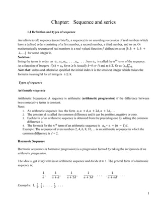
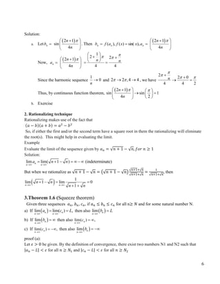
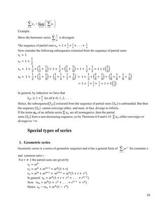
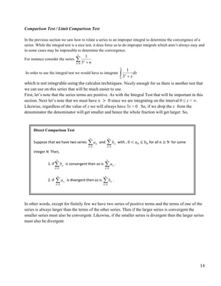
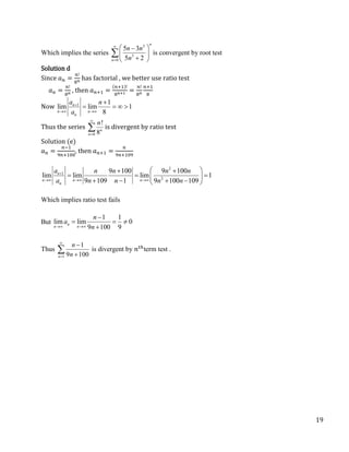
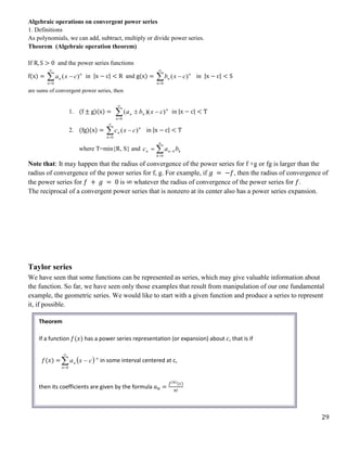
1.6 Alternating Series Test
The last two tests that we looked at for series convergence have required that the terms in the series
need to be positive except for finitely few first terms. Of course there are many series out there that
have negative terms in them and so we now need to start looking at tests for these kinds of series.
The test that we are going to look into in this section will be a test for alternating series. An
alternating series is any series, n
a
 , series with both positive and negative terms, but in a regular
pattern . Or any series n
a
 for which the series terms can be written in one of the following two
forms.
𝑎𝑛 = (−1)𝑛
𝑏𝑛 or 𝑎𝑛 = (−1)𝑛+1
𝑏𝑛, where 𝑏𝑛 ≥ 0
Suppose that we have a series ∑ 𝑎𝑛 and either 𝑎𝑛 = (−1)𝑛
𝑏𝑛 or where 𝑎𝑛 = (−1)𝑛+1
𝑏𝑛 for all
n. Then if
lim 0
n
n
b

 and {𝑏𝑛} is a decreasing sequence, the series ∑ 𝑎𝑛 is convergent.
.1.7 Absolute and conditional convergence
Roughly speaking there are two ways for a series to converge: As in the case of P 

1
2
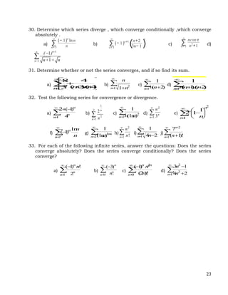
1
n n
, the
individual terms get small very quickly, so that the sum of all of them stays finite, or, as in the case of





1
1
)
1
(
n
n
n
, the terms don’t get small fast enough ( 

1
1
n n
diverges), but a mixture of positive and
negative terms provides enough cancellation to keep the sum finite. You might guess from what we’ve
seen that if the terms get small fast enough to do the job, then whether or not some terms are negative
and some positive the series converges.
A series  n
a is said to converge absolutely if  n
a is convergent; to say that  n
a converges
absolutely is to say that any cancellation that happens to come along is not really needed, as the terms
already get small so fast that convergence is guaranteed by that alone.
A series  n
a is said to converge conditionally if  n
a converges but  n
a diverges.
THEOREM If  n
a converges, then  n
a converges.
Proof: 0 ≤ an + |an| ≤ 2|an| so by the comparison test ∑(an + |an|) converges.
∑(an + |an|) − ∑|𝑎𝑛| = ∑[(an + |an|) − |an|] = ∑ an Converges by theorem

17. 17
1.8 Generalized convergence tests
Ratio Test
In this section we are going to take a look at a test that we can use to see if a series is absolutely
convergent or not. Recall that if a series is absolutely convergent then we will also know that it’s
convergent and so we will often use it to simply determine the convergence of a series.
Before proceeding with the test let’s do a quick reminder of factorials. This test will be particularly
useful for series that contain factorials.
Root Test
This is the last test for series convergence that we’re going to be looking at. As with the Ratio Test
this test will also tell whether a series is absolutely convergent or not rather than simple convergence.
Suppose that we have the series ∑ 𝑎𝑛 . Define,
1
lim lim
n n
n n
n n
L a a
 
 
Then,
1. If 𝐿 < 1 the series is absolutely convergent (and hence convergent).
2. If 𝐿 > 1 the series is divergent.
3. If 𝐿 = 1 the series may be divergent, conditionally convergent, or absolutely convergent.
Suppose we have the series . Define then,
1. If 𝐿 < 1 the series is absolutely convergent (and hence convergent).
2. If 𝐿 > 1 the series is divergent.
3. If 𝐿 = 1 the series may be divergent, conditionally convergent, or absolutely
convergent.

18. 18
Finally, we need to assume that 𝐿 = 1 and show that we could get a series that has any of the three
possibilities. To do this we just need a series for each case. We’ll leave the details of checking to you
but all three of the following series have 𝐿 = 1 and each one exhibits one of the possibilities.
2
1
1
n n


 absolutely convergent
1
( 1)n
n n



 conditionally convergent
1
1
n n


 divergent
Example: Determine if each of the following series is convergent or divergent.
a) 2 1
1
( 10)
4 ( 1)
n
n
n n





 b) 1
1
( 9)
2
n
n
n n




 c)
3
3
0
5 3
5 2
n
n
n n
n


 

 

 
 d)
0
!
8n
n
n


 e)
1
1
9 100
n
n
n





Solution a
𝑎𝑛 =
(−10)𝑛
42𝑛+1(𝑛+1)
, then 𝑎𝑛+1 =
(−10)𝑛+1
42𝑛+3(𝑛+2)
Using ratio test we have
1 2 1 2 1
1
2 3 2 1
( 10) 4 ( 1) 10(10 ) 4 1
lim lim lim
4 ( 2) ( 10) 10 16(4 ) 2
n n n n
n
n n n n
n n n
n
a n n
a n n
  

 
  
 
  
   
  
 
=
10
16
< 1
Thus 2 1
1
( 10)
4 ( 1)
n
n
n n





 is absolutely convergent by ratio test
Solution b
𝑎𝑛 =
(−9)𝑛
2𝑛+1(𝑛)
, then 𝑎𝑛+1 =
(−9)𝑛+1
2𝑛+1(𝑛+1)
Using ratio test we have
1
1
1
( 9) 2 9(9 ) 2 9
lim lim lim 1
2 ( 1) ( 9) 9 2(2 ) 1 2
n n n n
n
n n n n
n n n
n
a n n
a n n



  
 

   
 
  
 
Thus 1
1
( 9)
2
n
n
n n




 is divergent by ratio test
Solution c
Since 𝑎𝑛 = (
5𝑛−3𝑛3
5𝑛3+2
)
𝑛
is a power function, we better use root test
1/
3 3
1/
3 3
5 3 5 3 3
lim lim lim 1
5 2 5 2 5
n
n
n
n
n n n
n n n n
a
n n
  
 
 
   
 
 
 

19. 19
Which implies the series
3
3
0
5 3
5 2
n
n
n n
n


 

 

 
 is convergent by root test
Solution d
Since 𝑎𝑛 =
𝑛!
8𝑛 has factorial , we better use ratio test
𝑎𝑛 =
𝑛!
8𝑛
, then 𝑎𝑛+1 =
(𝑛+1)!
8𝑛+1
=
𝑛!
8𝑛
𝑛+1
8
Now 1 1
lim lim 1
8
n
n n
n
a n
a

 

   
Thus the series
0
!
8n
n
n


 is divergent by ratio test
Solution (e)
𝑎𝑛 =
𝑛−1
9𝑛+100
, then 𝑎𝑛+1 =
𝑛
9𝑛+109
2
1
2
9 100 9 100
lim lim lim 1
9 109 1 9 100 109
n
n n n
n
a n n n n
a n n n n

  
 
 
  
 
   
 
Which implies ratio test fails
But
1 1
lim lim 0
9 100 9
n
n n
n
a
n
 

  

Thus
1
1
9 100
n
n
n




 is divergent by 𝑛𝑡ℎ
term test .

20. 20
Applied Mathematics II Worksheet one
1. Let be the sequence for which 1 6
a = and 1 6
n+ n
a = +a for n≥ 1 .
a) Find the first three terms of the sequence.
b) Show the sequence converges and find its limit.
2. Let a1 and k be any positive real numbers and let {an} be the sequence for
which an+1=
1
2
(an+
k
an
) for n≥ 1 .Assuming that this sequence converges, find its
limit.
3. Evaluate the following limit a) ln
lim
n
n n

b) 1
lim
n
( n+ n )


4. Evaluate the ff limits. a) lim
n→∞
(1+
0.05
n )
n
b) lim
n→∞
arcsin(1
√
2
cos
1
n) c) lim
n→∞
∫
−
1
n
1
n
ex
dx
5. Prove the following
a)
lim
n→∞
c
1
n
= 1 for any fixed c>0
. b) lim 0 1
p
n
n
n
= for any fixed p and c >
c

.
c)
lim
n→∞
cn
n !
= 0 for any fixed c>0
. d)
lim
n→∞
(1+
x
n)
n
= ex
for any fixed x
.
e)
 
ln
0
lim
p
k
n
n
= o for any fixed k >
n

6. If the sequence {an}n= 1 is defined as a1= 1 and an= an− 1+
1
2n for all n≥ 2 , then
the value of a101= ___________________.
7. Given
lim
n→∞
an= α
and a1= 1 , we define a new sequence bn=
1
2n
+(an− an+1 ) , then
∑
n= 1
∞
bn= ____________.
8. Prove that the ff sequences converge. a) sn =
2 4 ... 2n
3 5 ... 2n 1
( )
( + )
  
  
b) sn =
1 3 ... 2n 1
2 4 ... 2n
( )
( )
   
  
9. Let sn = ∫
0
n
e− x2
dx . Prove that {sn} converges.
10. Determine whether {sn} converges or diverges. If it converges, find its limit.
{an}

21. 21
a) sn =
2 2
2n 2
2n 1 1
n +
n

 
b) sn = 2
1
n
c) sn = 1
3 1
3 3
n
n n 


11. Prove that i) lim
n→∞
n!
nn = 0 ii) lim
n→∞
an
n! = 0 for every real number a
iii)
lim
n→∞
n
en
= 0
iv)
lim
n→∞
ln n
n
= 0
12. Let  be any real number. Determine the convergence or divergence of the
sequence 1
n
α
+
n
 
 
 
 
 
 
 
 
 
 
 
.
13. Let {an} be a sequence defined by an=
1
n+1
+
1
n+2
+…+
1
2n .
a) Find
a4− a5 . b) Show that {an} converges.
14. Determine whether the sequence
1
sin
n=
π
n
n

 
 
 
converges or diverges.
15. Determine if the following sequences are monotonic and/or bounded.
a) {− n2
}n= 0
∞
b) {(− 1)n+1
}n= 1
∞
c) 2
5
2
n=
n

 
 
 
16. Show that
1
1 2 3 2n 1
n=
( )
n !

 
   
 
 
is an increasing sequence.
17. Compute the 4th partial sum of each series a)
∑
n= 1
∞
(− 1)n
b)
∑
n= 1
∞
(
1
5
)n
c)
∑
n= 2
∞
(− 1)n
n
18. Find a formula for the partial sums of the seies . For each series, determine
the partial sums have a limit. If so, find the sum of the series.
a) ∑
n= 1
∞
(
1
3
)n
b) 2
1
1
9n 3n 2
n= ( + )


 c) ∑
n= 1
∞
4
n+2
5n− 1 d)
2
1
1
n=
n+ n
n +n



19. Show that

22. 22
i)
∑
n= 1
∞
ln(1−
1
n2
)= − ln 2
ii)
1
1.3
+
1
3.5
+
1
5.7
+...=
1
2 iii)
∑
n= 1
∞
6n
(3n+1
− 2n+1
)(3n
− 2n
)
= 2
20. Use the divergence test to show that the series diverges.
a)
1
2
3n 4
n=
n+
+

 b) ∑
n= 1
∞
arctann c) ∑
n= 1
∞
e
n
n
21. Find the sum of the following series.
a)
1
7 6
3 3 4
n
n=
+
(n+ )(n+ )

 
 
 
 b) 2 1
1
7 6
1 10n
n= n


 

 

 
 .
22. Prove that
2
1
ln p
n= n( n)

 converges for p>1 and diverges for p≤ 1 .
23. Determine those value(s) of p for which the series ∑
n= 1
∞
1
(n+2)p2
− p+1 converges.
24. Check the convergence or the divergence of the following series.
a) ∑
n= 1
∞
arctann
n2
+1 b) ∑
n= 1
∞
n2
en− 3
c) ∑
n= 1
∞
1
9n2
+1
25. Use the comparison test or limit comparison test and determine the
convergence or divergence of the following series. a) ∑
n= 1
∞
n
n3
+1 b) ∑
n= 2
∞
1
n√
n2
− 1
c)
∑
n= 1
∞
1
en2 d) 2
1 3
n=
n
n



26. Determine whether the following series converges or diverges.
a)
1 2n
n=
n!

 b)
1 2n
n=
n!
( )!

 c)
1
2n
2n n
n=
( )!
n!( )

 d)
1
1.3.5.7.... 2n 1
2.4.6.8..... 2n
n=
( )
( )



e) ∑
n= 1
∞
ln n
en f) ∑
n= 1
∞
n(
π
4
)n
g) ∑
n= 1
∞
(
n
2n+5
)n
27. If ∑
n= 1
∞
an is absolutely convergent, must ∑
n= 1
∞
(an+an+1) be absolutely convergent?
Explain your answer.
28. Determine whether the series converges or diverges .
a)
1
1
1
4n
n
n=
n+
( )


 b)
2
1
ln
1 n
n=
( n)
( )
n


 c) 1
1
1
100
n+
n
n=
n!
( )


 d)
1
1
1 cot
2
n
n=
π
( )
n

 
 
 
 

29. For which positive values of p does the series ∑
n= 1
∞
(− 1)n 1
np converge?

23. 23
30. Determine which series diverge , which converge conditionally ,which converge
absolutely .
a) ∑
n= 3
∞
(− 1)n
ln n
n b) ∑
n= 3
∞
(− 1)n+1
(n+2
3n− 1 )
n
c) ∑
n= 3
∞
nconπ
n2
+1 d)
1
3
1
1
n+
n=
( )
n+ + n



31. Determine whether or not the series converges, and if so find its sum.
a) b) c) d)
32. Test the following series for convergence or divergence.
a) b) c) d) e)
f) g) h) i) j)
33. For each of the following infinite series, answer the questions: Does the series
converge absolutely? Does the series converge conditionally? Does the series
converge?
a) b) c) d)












1 )
4
)(
3
(
4
3
8
n
n
n
n


 
1
2
1
n n
n


 
1 )
2
(
1
n n
n


 

1 )
2
)(
1
(
1
n n
n
n





1 4
)
1
(
2
n
n
n


1
2
1
2
n
n
n



2
2
)
(ln
1
n n
n


1
2
3
n
n
n










1
2
1
1
2
n
n
n
n




2
ln
)
1
(
n
n
n
n



2
ln
)
(ln
1
n
n
n


1
2
!
n n
n


 
1 2
4
1
n n





1
2
!
)
1
(
7
n
n
n




1 2
!
)
1
(
n
n
n
n




0 !
)
3
(
n
n
n




0
2
!
)
2
(
)
1
(
n
n
n
n



 

1
2
2
2
4
1
3
n n
n

24. 24
Chapter 2 Power series
2.1 Definition of power series at any center c and center c = 0
A power series about c, or just power series, is any series that can be written in the form,
 




0
n
n
n c
x
a where 𝑥 is a variable, whereas c and 𝑎𝑛’s are real constants.
The 𝑎𝑛’s are often called the coefficients of the series and c the center of the series. If 𝑐 = 0, the series
becomes 

0
n
n
n x
a and is called power series center at zero.
2.2 Convergence and divergence, radius and interval of convergence
For each fixed value of 𝑥, the series  




0
n
n
n c
x
a is a series of constants that we can test for
convergence or divergence. A power series may converge for some values of 𝑥 and diverge for other
values of 𝑥.
Theorem(convergence theorem for power series)
If a power series  




0
n
n
n c
x
a is convergent at a point x = r + 𝑐 for 𝑟 > 0, then it is absolutely
convergent at every point of the interval (𝑐– 𝑟, 𝑐 + 𝑟).
Radius and interval of convergence
The maximum value of r of the theorem above written as R for which the power series is convergent in
the interval (c–R, c+ R) is called the radius of convergence of the power series.
.
For a given power series there are only three possibilities:
(i) The series converges at the center only (𝑖. 𝑒 when 𝑥 = 𝑐). Here 𝑅 = 0
(ii) The series converges for all 𝑥. Here 𝑅 = ∞
(iii) There is a positive number 𝑅 such that the series converges absolutely if |𝑥 − 𝑐| < 𝑅 and
diverges if |𝑥 − 𝑐| > 𝑅

25. 25
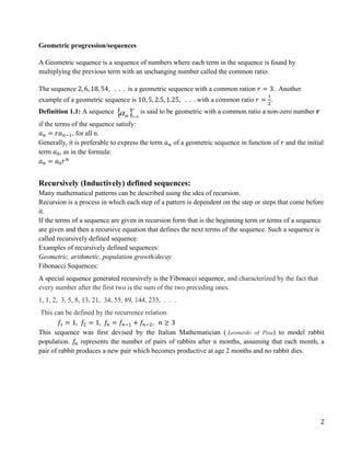
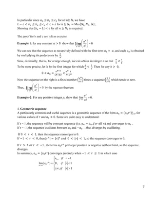
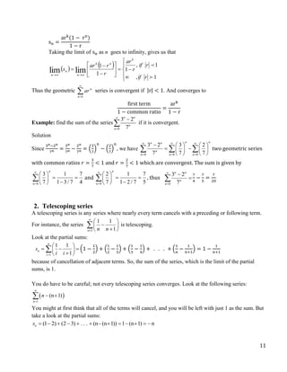
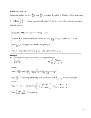
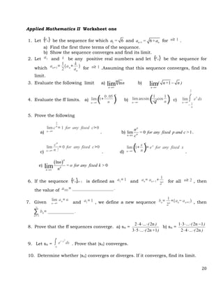
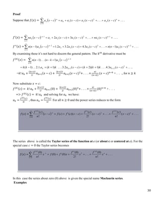
The interval of convergence of a power series is the interval that consists of all values of 𝑥 for which
the series converges.
In case (i) the interval consists of just a single point c (𝑖. 𝑒 [𝑐, 𝑐] = {𝑐}),
In case (ii) the interval is (−∞, ∞),
In case (iii) there are four possibilities for the interval of convergence:
(𝑐 − 𝑅, 𝑐 + 𝑅), (𝑐 − 𝑅, 𝑐 + 𝑅], [𝑐 − 𝑅, 𝑐 + 𝑅), [𝑐 − 𝑅, 𝑐 + 𝑅]
Therefore, to completely identify the interval of convergence of case (iii), all that we have to do is determine if
the power series will converge for 𝑥 = 𝑐 −R or 𝑥 = 𝑐 + 𝑅 and is called end point convergence test. If the
power series converges for one or both of these values then we’ll need to include those in the interval of
convergence.
Remark
1. The power series defines a real-valued function at any point x in its interval of convergence.
2. The Ratio Test can be used to determine the radius of convergence in most cases. The Ratio test
always fails when 𝑥 is an endpoint of the interval of convergence of case (iii), so the endpoints
must be checked with some other test.
Examples
For each of the following power series determine the radius and interval of convergence.
1.
 




1
1
n
n
n
x
2. 

0 !
n
n
n
x
3. 

0
!
n
n
x
n
Solution-1
Take 𝑏𝑛 =
(𝑥−1)𝑛
𝑛
, then 𝑏𝑛+1 =
(𝑥−1)𝑛+1
𝑛+1
𝑏𝑛+1
𝑏𝑛
= (
(𝑥−1)𝑛+1
𝑛+1
)
𝑛
(𝑥−1)𝑛
=
𝑛
𝑛+1
(𝑥 − 1)
1
1
1
1
1 lim
lim
lim 1















x
n
n
x
x
n
n
b
b
n
n
n
n
n
By ratio test
 




1
1
n
n
n
x
is absolutely convergent if |𝑥 − 1| < 1 and divergent if |𝑥 − 1| > 1. This means that
the radius of convergence is 𝑅 = 1.
For the interval of convergence check at the end points (at 𝑥 = 0 and 𝑥 = 2)
At 𝑥 = 0,
 
 







1 1
)
1
(
1
n n
n
n
n
n
x
is convergent alternating series, hence convergent
At 𝑥 = 2,
 
 






1 1
1
1
n n
n
n
n
x
is divergent p-series, hence divergent
Thus the interval of convergence is 𝐼𝑅 = [0, 2).

26. 26
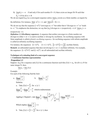
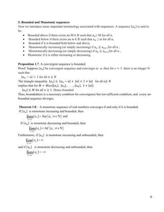
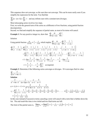
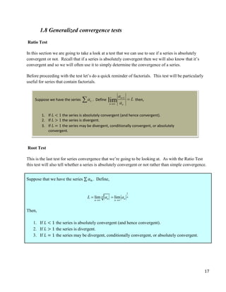
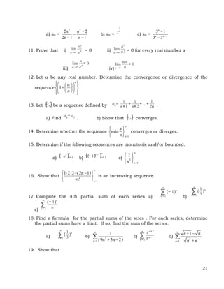
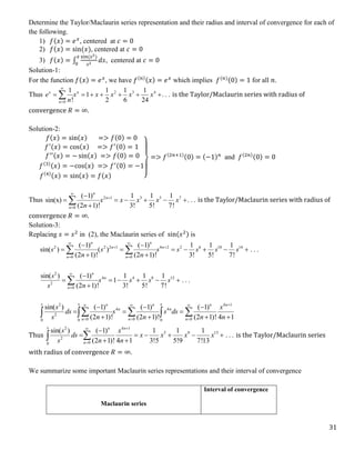
Solution-2
Take 𝑏𝑛 =
𝑥𝑛
𝑛!
, then 𝑏𝑛+1 =
𝑥𝑛+1
(𝑛+1)!
=
𝑥𝑛
𝑛!
𝑥
𝑛+1
𝑏𝑛+1
𝑏𝑛
= (
𝑥𝑛
𝑛!
𝑥
𝑛+1
)
𝑛!
𝑥𝑛
=
𝑥
𝑛+1
0
0
1
1
1 lim
lim
lim 1














x
n
x
n
x
b
b
n
n
n
n
n
< 1 for all 𝑥 ∈ ℝ
This means 

1 !
n
n
n
x
is absolutely convergent for all 𝑥 ∈ ℝ. Thus radius of convergence 𝑅 = ∞ and interval of
convergence 𝐼𝑅 = (−∞, ∞).
Solution-3
Take 𝑏𝑛 = 𝑛! 𝑥𝑛
, then 𝑏𝑛+1 = (𝑛 + 1)! 𝑥𝑛+1
= (𝑛 + 1)𝑛! 𝑥𝑛
𝑥
𝑏𝑛+1
𝑏𝑛
=
(𝑛+1)𝑛!𝑥𝑛𝑥
𝑛!𝑥𝑛 = (𝑛 + 1)𝑥













)
1
(
)
1
( lim
lim
lim 1
n
x
x
n
b
b
n
n
n
n
n
for 𝑥 ≠ 0
This means 

0
!
n
n
x
n is convergent for all 𝑥 = 0. Thus radius of convergence 𝑅 = 0 and interval of
convergence 𝐼𝑅 = [0,0]
Note that for a power series of the form  kn
n
n c
x
a 


0
the radius of convergence
𝑅 =
k
n
n
n a
a
1
1
lim 


for any positive k.
Representations of Functions as Power Series
In this section we learn how to represent certain types of functions as sums of power series by manipulating
geometric series or by differentiating or integrating such a series. You might wonder why we would ever want
to express a known function as a sum of infinitely many terms. We will see later that this strategy is useful for
integrating functions that don’t have elementary antiderivatives, for solving differential equations, and for
approximating functions by polynomials. (Scientists do this to simplify the expressions they deal with;
computer scientists do this to represent functions on calculators and computers.)
Geometric series
Consider the power series 

0
n
n
x = 1 + 𝑥 + 𝑥2
+ . . . + 𝑥𝑛
+ . . .
This is a geometric series with a common ratio 𝑟 = 𝑥 and first term =1. Hence the power series converges to
1
1−𝑥
, if |𝑥| < 1 and diverges if |𝑥| ≥ 1.
Now we say that the function 𝑓(𝑥) =
1
1−𝑥
has a power series representation of the form 

0
n
n
x for |𝑥| < 1 .
The radius of convergence 𝑅 = 1 and interval of convergence 𝐼𝑅 = (−1, 1) for this series.
Differentiation and Integration of Power Series.

27. 27
Since the sum of a power series is a function we can differentiate it and integrate it in its interval of
convergence. The result is another function that can also be represented with another power series. The main
related result is that the derivative or integral of a power series can be computed by term-by-term
differentiation and integration as can be done to polynomials:
The idea is that the geometrical decay of the terms of the power series inside its radius of convergence
dominates the algebraic growth of the factor n that comes from taking the derivative. And the geometrical
growth of the power series outside its radius of convergence dominates the algebraic decay that comes from
taking the integral.
Proof: To prove this result, we need to show that the term-by-term derivative of a power series has the same
radius of convergence as the original power series.
Assume without loss of generality that c = 0, and suppose |𝑥| < 𝑅. Choose 𝜌 such that |𝑥| < 𝜌 < 𝑅, and let
𝑟 =
|𝑥|
𝜌
, 0 < 𝑟 < 1
To estimate the terms in the differentiated power series by the terms in the original series, we rewrite their
absolute values as follows:
|𝑛𝑎𝑛𝑥𝑛−1| =
𝑛
𝜌
(
|𝑥|
𝜌
)
𝑛−1
|𝑎𝑛𝜌𝑛| =
𝑛𝑟𝑛−1
𝜌
|𝑎𝑛𝜌𝑛|
The ratio test shows that the series 



1
1
n
n
nr converges since 1
1
1
)
1
(
lim
lim 1





















 





r
r
n
nr
r
n
n
n
n
n
so the sequence {𝑛𝑟𝑛−1} is bounded, by M say. It follows that
|𝑛𝑎𝑛𝑥𝑛−1| =
𝑛𝑟𝑛−1
𝜌
|𝑎𝑛𝜌𝑛| ≤
𝑀
𝜌
|𝑎𝑛𝜌𝑛| for all 𝑛 ≥ 1.
The series 






1
1 n
n
n
n
n
n a
M
a
M




converges since 𝜌 < 𝑅, so the comparison test implies that




1
1
n
n
n x
na converges absolutely.
Conversely, suppose |𝑥| > 𝑅.
Theorem: If the power series  




0
n
n
n c
x
a has radius of convergence 𝑅 > 0, then the function
𝑓(𝑥) defined by 𝑓(𝑥) = 𝑎0 + 𝑎1(𝑥 − 𝑐) + 𝑎2(𝑥 − 𝑐)2
+ . . . =  




0
n
n
n c
x
a
is differentiable and integrable in the interval (c-R, c+R) and
i. 𝑓′(𝑥) = 𝑎1 + 2𝑎2(𝑥 − 𝑐) + 3𝑎3(𝑥 − 𝑐)2
+ . . . =  





1
1
n
n
n c
x
na ,
ii. ∫ 𝑓(𝑥)𝑑𝑥 = 𝐶 + 𝑎0(𝑥 − 𝑐) +
𝑎1
2
(𝑥 − 𝑐)2
+
𝑎2
3
(𝑥 − 𝑐)3
+ . . . = C+  






0
1
1
n
n
n
c
x
n
a
The radii of convergence of the power series in Equations (i) and (ii) are both R.

28. 28
Then 



1
1
n
n
n x
na diverges since 

0
n
n
n x
a diverges and |𝑛𝑎𝑛𝑥𝑛−1| ≥
1
|𝑥|
|𝑎𝑛𝑥𝑛| for 𝑛 ≥ 1.
Thus the series 



1
1
n
n
n x
na has a radius of convergence R the same as 

0
n
n
n x
a .
Power series representation of functions using Differentiation and Integration of Power Series
We have previously learned how to compute power series representations of certain functions, by relating
them to geometric series. We can obtain power series representation for a wider variety of functions by
exploiting the fact that a convergent power series can be differentiated, or integrated, term-by-term to obtain a
new power series that has the same radius of convergence as the original power series. The new power series
is a representation of the derivative, or anti-derivative, of the function that is represented by the original power
series.
This is particularly useful when we have a function 𝑓(𝑥) for which we do not know how to obtain a power
series representation directly. If its derivative 𝑓′(𝑥), or its anti-derivative ∫ 𝑓(𝑥)𝑑𝑥 is a function for which a
power series representation can easily be computed.
Example1 The function 𝑓(𝑥) =
4
(2−𝑥)2 is the derivative of the function 𝑔(𝑥) =
2𝑥
2−𝑥
But
2𝑥
2−𝑥
=



0
1
2
1
n
n
n
x which converges when |𝑥| < 2 = 𝑅
To obtain a power series representation of f(x), we differentiate this series term-by-term to obtain
4
(2−𝑥)2
=



0 2
1
n
n
n
x
n
which also converges when |𝑥| < 2 = 𝑅
Example2: Consider the definite integral dx
x
 
1
0
4
1
1
Attempting to evaluate this integral using partial fraction decomposition is not possible without introducing
complex numbers. Instead, we express the integrand as a (geometric) power series:
1
1+𝑥4
=
1
1−(−𝑥4)
=



0
4
)
1
(
n
n
n
x in the interval (-1, 1) which contains the interval of integration (0,1).
Integrating the power series term-by-term from 0 to 1 yields


 dx
x
1
0
4
1
1





dx
x
n
n
n
1
0 0
4
)
1
( 

 






 






0
1
0
1
4
0
0
1
0
4
1
4
)
1
(
1
4
)
1
(
)
1
(
n
n
n
n
n
n
n
n
n
x
n
dx
x
This is an alternating series, which, by the alternating series test converges.
Using the alternating series estimation theorem, we can evaluate this integral numerically, to any degree of
accuracy we wish, by choosing 𝑛 large enough so that
1
4𝑛+1
is sufficiently small.
Taking n=50, 

 dx
x
1
0
4
1
1
0.869436 with an error less than 0.00488

29. 29
Algebraic operations on convergent power series
1. Definitions
As polynomials, we can add, subtract, multiply or divide power series.
Theorem (Algebraic operation theorem)
If R, S > 0 and the power series functions
f(x) = 



0
)
(
n
n
n c
x
a in |x − c| < R and g(x) = 



0
)
(
n
n
n c
x
b in |x − c| < S
are sums of convergent power series, then
1. (f ± g)(x) = 




0
)
)(
(
n
n
n
n c
x
b
a in |x − c| < T
2. (fg)(x) = 



0
)
(
n
n
n c
x
c in |x − c| < T
where T=min{R, S} and 



n
k
k
k
n
n b
a
c
0
Note that: It may happen that the radius of convergence of the power series for f +g or fg is larger than the
radius of convergence of the power series for f, g. For example, if 𝑔 = −𝑓, then the radius of convergence of
the power series for 𝑓 + 𝑔 = 0 is ∞ whatever the radius of convergence of the power series for 𝑓.
The reciprocal of a convergent power series that is nonzero at its center also has a power series expansion.
Taylor series
We have seen that some functions can be represented as series, which may give valuable information about
the function. So far, we have seen only those examples that result from manipulation of our one fundamental
example, the geometric series. We would like to start with a given function and produce a series to represent
it, if possible.
Theorem
If a function 𝑓(𝑥) has a power series representation (or expansion) about 𝑐, that is if
𝑓(𝑥) =  




0
n
n
n c
x
a in some interval centered at c,
then its coefficients are given by the formula 𝑎𝑛 =
𝑓(𝑛)
(𝑐)
𝑛!

30. 30
Proof
Suppose that 𝑓(𝑥) =   .
.
.
)
(
.
.
.
)
(
)
( 2
2
1
0
0













n
n
n
n
n c
x
a
c
x
a
c
x
a
a
c
x
a
𝑓′(𝑥) =   .
.
.
)
(
.
.
.
)
(
3
)
(
2 1
2
3
2
1
1
1









 



 n
n
n
n
n c
x
na
c
x
a
c
x
a
a
c
x
na
𝑓′′(𝑥) =   .
.
.
)
(
)
1
(
.
.
.
)
(
3
.
4
)
(
2
.
3
2
.
1
)
1
( 2
2
4
3
2
2
2











 



 n
n
n
n
n c
x
a
n
n
c
x
a
c
x
a
a
c
x
a
n
n
By examining these it’s not hard to discern the general pattern. The 𝑘𝑡ℎ
derivative must be
𝑓(𝑘)(𝑥) =  








k
n
k
n
n c
x
a
k
n
n
n )
1
.(
.
.
)
1
(
.
.
.
.
)
(
3
.
4
.
.
.
)
1
)(
2
(
)
(
2
.
3
.
.
.
)
1
(
.
1
.
2
.
.
)
1
( 2
2
1 








 
 c
x
a
k
k
k
c
x
a
k
k
a
k
k k
k
k
=𝑘! 𝑎𝑘 +
(𝑘+1)!
1!
𝑎𝑘+1(𝑥 − 𝑐) +
(𝑘+2)!
2!
𝑎𝑘+2(𝑥 − 𝑐)2
+ . . . +
𝑛!
(𝑛−𝑘)!
(𝑥 − 𝑐)𝑛−𝑘
+ . . ., for 𝑛 ≥ 𝑘
Now substitute 𝑥 = 𝑐:
𝑓(𝑘)(𝑐) = 𝑘! 𝑎𝑘 +
(𝑘+1)!
1!
𝑎𝑘+1(0) +
(𝑘+2)!
2!
𝑎𝑘+2(0)2
+ . . . +
𝑛!
(𝑛−𝑘)!
(0)𝑛−𝑘
+ . . .
=> 𝑓(𝑘)(𝑐) = 𝑘! 𝑎𝑘 and solving for 𝑎𝑘 we have:
𝑎𝑘 =
𝑓(𝑘)(𝑐)
𝑘!
, thus 𝑎𝑛 =
𝑓(𝑛)(𝑐)
𝑛!
For all 𝑛 ≥ 0 and the power series reduces to the form
The series above is called the Taylor series of the function at c (or about c or centered at c). For the
special case 𝑐 = 0 the Taylor series becomes
In this case the series about zero (0) above is given the special name Maclaurin series.
Examples
𝑓(𝑥) =
𝑓(𝑥) =

31. 31
Determine the Taylor/Maclaurin series representation and their radius and interval of convergence for each of
the following.
1) 𝑓(𝑥) = 𝑒𝑥
, centered at 𝑐 = 0
2) 𝑓(𝑥) = sin(𝑥), centered at 𝑐 = 0
3) 𝑓(𝑥) = ∫
sin(𝑠2)
𝑠2
𝑑𝑠
𝑥
0
, centered at 𝑐 = 0
Solution-1:
For the function 𝑓(𝑥) = 𝑒𝑥
, we have 𝑓(𝑛)
(𝑥) = 𝑒𝑥
which implies 𝑓(𝑛)(0) = 1 for all 𝑛.
Thus 2 3 4
0
1 1 1 1
1 . . .
! 2 6 24
x n
n
e x x x x x
n


      
 is the Taylor/Maclaurin series with radius of
convergence 𝑅 = ∞.
Solution-2:
𝑓(𝑥) = sin(𝑥) => 𝑓(0) = 0
𝑓′(𝑥) = cos(𝑥) => 𝑓′(0) = 1
𝑓′′(𝑥) = − sin(𝑥) => 𝑓(0) = 0
𝑓(3)
(𝑥) = −cos(𝑥) => 𝑓′(0) = −1
𝑓(4)
(𝑥) = sin(𝑥) = 𝑓(𝑥) }
=> 𝑓(2𝑛+1)
(0) = (−1)𝑛
and 𝑓(2𝑛)
(0) = 0
Thus 2 1 3 5 7
0
( 1) 1 1 1
sin(x) . . .
(2 1)! 3! 5! 7!
n
n
n
x x x x x
n




     

 is the Taylor/Maclaurin series with radius of
convergence 𝑅 = ∞.
Solution-3:
Replacing 𝑠 = 𝑠2
in (2), the Maclaurin series of sin(𝑠2) is
2 2 2 1 4 2 2 6 10 14
0 0
( 1) ( 1) 1 1 1
sin( ) ( ) . . .
(2 1)! (2 1)! 3! 5! 7!
n n
n n
n n
s s s s s s s
n n
 
 
 
 
      
 
 
2
4 4 8 12
2
0
sin( ) ( 1) 1 1 1
1 . . .
(2 1)! 3! 5! 7!
n
n
n
s
s s s s
s n



     


2 4 1
4 4
2
0 0 0
0 0 0
sin( ) ( 1) ( 1) ( 1)
(2 1)! (2 1)! (2 1)! 4 1
x x x
n n n n
n n
n n n
s x
ds s s ds
s n n n n

  
  
  
  
   
  
  
Thus
2 4 1
5 9 13
2
0
0
sin( ) ( 1) 1 1 1
. . .
(2 1)! 4 1 3!5 5!9 7!13
x n n
n
s x
ds x x x x
s n n




     
 

 is the Taylor/Maclaurin series
with radius of convergence 𝑅 = ∞.
We summarize some important Maclaurin series representations and their interval of convergence
Maclaurin series
Interval of convergence

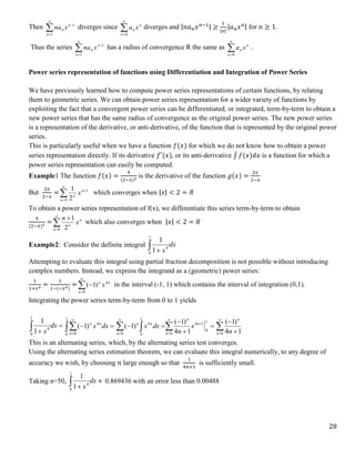
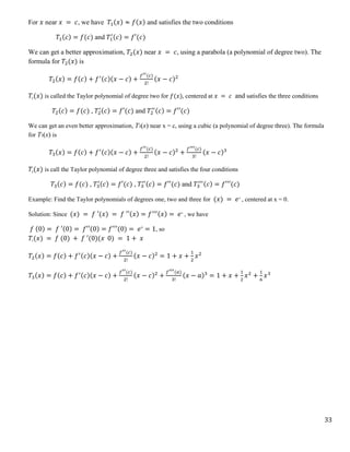
32. 32
2 3
0
1 . . .
2! 3! !
n
x
n
x x x
e x
n


      
(−∞, ∞)
2 4 6
2
0
( 1)
cos( ) 1 . . .
2! 4! 6! (2 )!
n
n
n
x x x
x x
n



      
(−∞, ∞)
3 5 7
2 1
0
( 1)
sin( ) . . .
3! 5! 7! (2 1)!
n
n
n
x x x
x x x
n




     


(−∞, ∞)
3 5 7
1 2 1
0
( 1)
tan ( ) . . .
3 5 7 2 1
n
n
n
x x x
x x x
n

 


     


[−1, 1]
2 4 6 2
0
cosh( ) 1 . . .
2! 4! 6! (2 )!
n
n
x x x x
x
n


      
(−∞, ∞)
3 5 7 2 1
0
sinh( ) . . .
3! 5! 7! (2 1)!
n
n
x x x x
x x
n



     


(−∞, ∞)
2 3 4
1
0
( 1)
ln(1 ) . . .
2 3 4 1
n
n
n
x x x
x x x
n




      


(−1, 1]
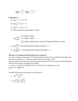
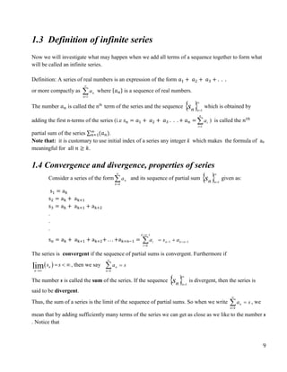
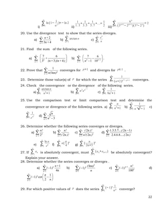
Taylor polynomials
Idea of a Taylor polynomial
Polynomials are simpler than most other functions. This leads to the idea of approximating a complicated
function by a polynomial. Taylor realized that this is possible provided there is an “easy” point at which you
know how to compute the function and its derivatives. Given a function f(x) and a value c, we will define for
each degree n a polynomial Tn(x) which is the “best nth
degree polynomial approximation to f(x) near x = c.
𝑇0(𝑥) = 𝑓(𝑐) ……. the zero degree Taylor polynomial
𝑇1(𝑥) = 𝑓(𝑐) + 𝑓′(𝑐)(𝑥 − 𝑐)
𝑇1(𝑥) is called the Taylor polynomial of degree one for 𝑓(𝑥), centered at 𝑥 = 𝑐 and is also tangent to the graph
𝑓(𝑥) at 𝑥 = 𝑐.

33. 33
For 𝑥 near 𝑥 = 𝑐, we have 𝑇1(𝑥) ≈ 𝑓(𝑥) and satisfies the two conditions
𝑇1(𝑐) = 𝑓(𝑐) and 𝑇1
′(𝑐) = 𝑓′(𝑐)
We can get a better approximation, 𝑇2(𝑥) near 𝑥 = 𝑐, using a parabola (a polynomial of degree two). The
formula for 𝑇2(𝑥) is
𝑇2(𝑥) = 𝑓(𝑐) + 𝑓′(𝑐)(𝑥 − 𝑐) +
𝑓′′(𝑐)
2!
(𝑥 − 𝑐)2
𝑇2(𝑥) is called the Taylor polynomial of degree two for 𝑓(𝑥), centered at 𝑥 = 𝑐 and satisfies the three conditions
𝑇2(𝑐) = 𝑓(𝑐) , 𝑇2
′(𝑐) = 𝑓′(𝑐) and 𝑇2
′′(𝑐) = 𝑓′′(𝑐)
We can get an even better approximation, T3(x) near x = c, using a cubic (a polynomial of degree three). The formula
for T3(x) is
𝑇3(𝑥) = 𝑓(𝑐) + 𝑓′(𝑐)(𝑥 − 𝑐) +
𝑓′′(𝑐)
2!
(𝑥 − 𝑐)2
+
𝑓′′′(𝑐)
3!
(𝑥 − 𝑐)3
𝑇3(𝑥) is call the Taylor polynomial of degree three and satisfies the four conditions
𝑇3(𝑐) = 𝑓(𝑐) , 𝑇3
′(𝑐) = 𝑓′(𝑐) , 𝑇3
′′(𝑐) = 𝑓′′(𝑐) and 𝑇3
′′′(𝑐) = 𝑓′′′(𝑐)
Example: Find the Taylor polynomials of degrees one, two and three for (𝑥) = 𝑒𝑥
, centered at x = 0.
Solution: Since (𝑥) = 𝑓 ′(𝑥) = 𝑓 ′′(𝑥) = 𝑓′′′(𝑥) = 𝑒𝑥
, we have
𝑓 (0) = 𝑓 ′(0) = 𝑓′′(0) = 𝑓′′′(0) = 𝑒0
= 1, so
𝑇1(𝑥) = 𝑓 (0) + 𝑓 ′(0)(𝑥 0) = 1 + 𝑥
𝑇2(𝑥) = 𝑓(𝑐) + 𝑓′(𝑐)(𝑥 − 𝑐) +
𝑓′′(𝑐)
2!
(𝑥 − 𝑐)2
= 1 + 𝑥 +
1
2
𝑥2
𝑇3(𝑥) = 𝑓(𝑐) + 𝑓′(𝑐)(𝑥 − 𝑐) +
𝑓′′(𝑐)
2!
(𝑥 − 𝑐)2
+
𝑓′′′(𝑎)
3!
(𝑥 − 𝑎)3
= 1 + 𝑥 +
1
2
𝑥2
+
1
6
𝑥3

34. 34
In general, the Taylor polynomial of degree 𝑛 for 𝑓(𝑥), centered at 𝑥 = 𝑎, is
𝑇𝑛(𝑥) = 𝑓(𝑐) + 𝑓′(𝑐)(𝑥 − 𝑐) +
𝑓′′
(𝑐)
2!
(𝑥 − 𝑐)2
+
𝑓′′′
(𝑐)
3!
(𝑥 − 𝑐)3
+ . . . +
𝑓(𝑛)
(𝑐)
𝑛!
(𝑥 − 𝑐)𝑛
The formula for 𝑇𝑛(𝑥) can be written using summation notation:
( )
0
(c)
( ) ( )
!
k
n
k
n
k
f
T x x c
k

 

By a similar computation to that for T2(x) or for T3(x) , it can be shown that Tn(x) satisfies the n + 1 conditions
𝑇𝑛(𝑐) = 𝑓(𝑐), 𝑇𝑛
′(𝑐) = 𝑓′(𝑐), 𝑇𝑛
′′(𝑐) = 𝑓′′(𝑐), . . . , 𝑇𝑛
(𝑛)
(𝑐) = 𝑓(𝑛)
(𝑐)
Taylor's Theorem
Suppose that 𝑓 is defined on some open interval I around c and suppose 𝑓(𝑁+1)
(𝑥) exists on this interval.
Then for each 𝑥 ≠ 𝑐 in I there is a value 𝑧 between 𝑥 and 𝑐 so that
1
)
1
(
0
)
(
)
(
!
)
1
(
)
(
)
(
!
)
(
)
( 






  N
N
n
N
n
n
c
x
N
z
f
c
x
n
c
f
x
f , for some 𝑧 between 𝑥 and 𝑐
Note that: In the Taylor theorem
( ) ( 1)
1
0
( ) ( )
( ) ( ) ( )
! ( 1)!
n N
N
n N
n
f c f z
f x x c x c
n N



   


The portion 𝑇𝑛(𝑥) =
( )
0
( )
( )
!
n
N
n
n
f c
x c
n


 is said to be Taylors polynomial of degree 𝑛 and the portion 𝑅𝑛 =
( 1)
1
( )
( )
( 1)!
N
N
f z
x c
N




is the remainder , thus
𝑓(𝑥) = 𝑇𝑛(𝑥) + 𝑅𝑛
Example: approximate 𝑒−0.2
using Taylor series with an error less than 0.0001.
Solution
Take the Taylor polynomial of 𝑒𝑥

35. 35
2 3
1 . . .
2! 3! !
n
x
n
x x x
e x R
n
       , here
( 1)
1
( )
( 1)!
n
n
n
f z
R x
n




,for some 𝑧 between 0 & 𝑥.
For 𝑥 = −0.2,
1
1 (0.2)
( 0.2) ,
( 1)! ( 1)!
z n
n
n
e
R
n n


  
 
−0.2 < 𝑧 < 0
If we take 𝑛 = 3,
4
4
3
(0.2)
( 0.2) 0.00006667
4! 24
z
e
R     < 0.0001
Thus
2 3
0.2 ( 0.2) ( 0.2)
1 0.2
2
0.818666667
6
e  
    
Work sheet on Chapter two (Power series)
1. Determine the interval of convergence for each of the following series
a) 

 
1
2
1
n
n
n
x
b) 

 


1
2
)
1
(
)
4
(
)
1
(
n
n
n
n
x
c) 



1
)
3
)(
(ln
n
n
n
x
n
d) 



1
2
4
)
3
2
(
n
n
n
x
e)


 

1
2
)!
1
2
(
)
1
(
n
n
n
n
x

2. Find the radius of convergence of the power series n
n
x
q
n
n
p
n


 

1 )!
(
!
)!
(
where p and q are
positive integers.
3. If k is positive integer , find the radius of the series
 


0 )!
(
!
n
n
k
kn
x
n
4. Prove that if n
n
n
c
1
lim


= L , then
L
1
is the radius of convergence of the power series


1
n
n
n x
c

36. 36
5. Let )
(x
f = n
n
n
x
n
2
0 )!
2
(
)
1
(




and 
)
(x
g 1
2
0 )!
1
2
(
)
1
( 


 
 n
n
n
x
n
a. Show that )
(
)
(
,
x
g
x
f 
 and )
(
)
(
,
x
f
x
g 
b. Show that )
(
)
(
,
,
x
f
x
f 
 and )
(
)
(
,
,
x
g
x
g 

c. What functions do you know that satisfy the properties of (a) and (b).
d. Find the radius of convergence f(x) and g(x).
6. Find the power series representation for the following function and find the interval of
convergence
a. 2
9
1
1
)
(
x
x
f

 b.
x
x
x
f
4
1
)
(

 c. 3
3
2
)
(
x
a
x
x
f

 d. )
1
ln(
)
( 2
x
x
f 
 e. )
5
ln(
)
( x
x
f 

f. 2
2
)
2
1
(
)
(
x
x
x
f

 g. 2
3
)
2
(
)
(


x
x
x
f h. )
6
arctan(
)
(
x
x
f  i.
1
2
)
( 2


x
x
x
f j. 2
3
2
)
1
(
3
)
(
x
x
x
f


l.
2
1
)
( 2



x
x
x
f m. )
(
cos
)
( 2
x
x
f 
7. Show that if the radius of convergence of n
n
n x
c


0
is R , then
R
c
c
n
n
n
1
lim 1




.
8. Express the following integral as infinite series.
a.  
dt
t
t
8
1
b. 

dt
t
t)
1
ln(
c. 


dx
x
x
x
2
1
tan
d. dx
x )
(
tan 2
1


9. Find the Taylor series of f about the given point a .
a)
x
x
f
1
)
(  , 1


a b) 3
;
ln
)
( 
 a
x
x
f c) x
x
f 
)
( , 1

a
d) 1
;
3
ln
)
( 
 a
x
x
f e) 0
;
3
sin
)
( 
 a
x
x
f
10. Find the fourth Taylor polynomial of the given function about a.
a) 1
;
2
)
( 4




 a
x
x
x
f b)
3
;
arctan
)
(


 a
x
x
k c) 1
;
tan
)
( 
 a
x
x
f
11. Find the Maclaurin’s series of f where
a) x
x
f 4
cos
)
( 2
 b) x
e
x
f x
cos
)
(  c)
1
1
)
(



x
x
x
f
d)
1
3
2
2
3
)
( 2





x
x
x
x
f e) x
x
f 3
sinh
)
( 
12. Let x
x
f tan
)
(  . Using the fact that 0
)
0
( 
f and 2
)]
(
[
1
)
( x
f
x
f 

 , find the
sum of the first six terms in the Taylor series of f about 0.

37. 37
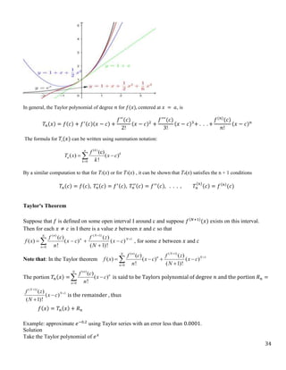
13. Use Taylor polynomials to approximate the number with an error less
than 0.001
a) 95 b) 3
1

e c)
5
sin

d) 4
17
14. Find the second Taylor polynomial of 4
1
)
( x
x
f 
 about 0.
15. Let ]
0
,
1
[
;
4
,
0
;
)
( 2



 n
a
e
x
f
x
. Then find
a) )
(
4 x
T at a
x  b) )
(
4 x
R at a
x 
c) an upper bound on the absolute value of the error if )
(x
f is
approximated over the given interval by the Taylor polynomial obtained in
part (a).