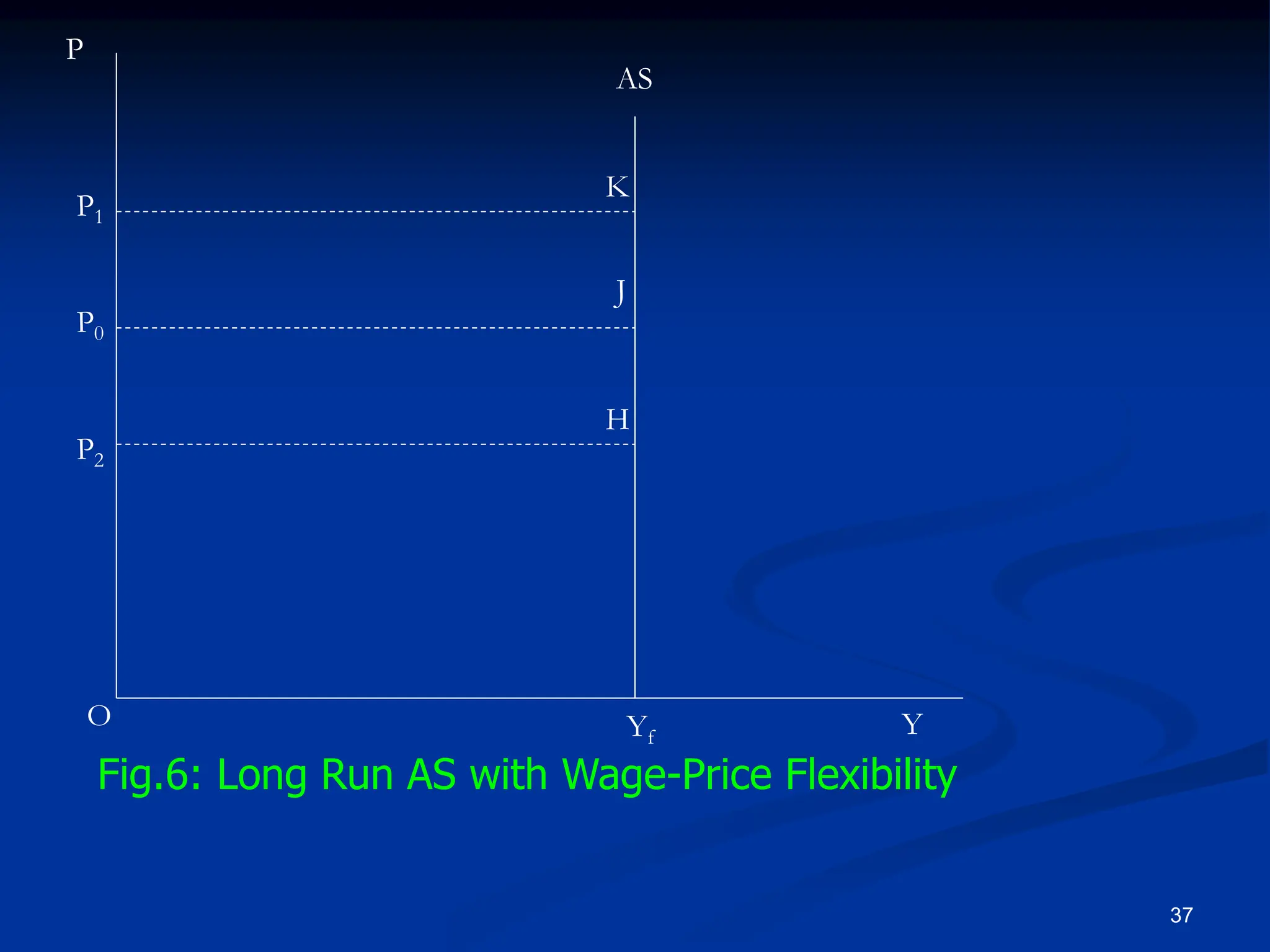
The aggregate supply curve is derived from the production function and factor markets. In the short run, the AS curve can be upward sloping under wage rigidity or perfectly elastic under price rigidity. In the long run, with wage-price flexibility, the AS curve is perfectly inelastic as output is constant at the full employment level, while money wages and prices adjust to maintain full employment.

1. 1
Chapter V
Production Function and
Aggregate Supply

2. 2
• Like the supply curve of an individual firm, the
aggregate supply curve is derived from the
production function.
• Given the technology level, the factors of
production determine the production function or
production relationships.
• The industry supply curve is derived from the
supply curves of individual firms through an
aggregation process.
• The industry supply curve shows the quantity of
output a particular industry is willing to supply at
different prices of the product.

3. 3
• The aggregate supply curve depicts the quantity
of all goods and services, which all industries in
the economy together, that is, at an aggregate
level, are willing to supply at different general
price levels.
• Both the industry and aggregate supply curves
are upward sloping under all normal
circumstances.

4. 4
5.1 Production Function
• A production function specifies the relationship
between inputs and outputs whether at micro
level or macro or aggregate level.
• But the inputs are not raw material inputs which
are consumed in the production process, but,
factor inputs which contribute to productivity and
value addition.
• So, a production function specifies the relationship
between factor inputs or factors of production,
and, output, given certain technology level.
• In macroeconomic analysis, output is represented
by income (Y).

5. 5
• The factors of production are land, labor, capital
and organization or enterprise or
entrepreneurship.
• As land, which is a natural resource, is mostly
fixed, it is not generally considered as a factor for
explaining changes in output or production.
• For simplicity, organization or entrepreneurship is
often combined with labor input (although income
of organization or entrepreneurship is profit not
wages).
• Then the production function of an economy, for a
given technology level, can be stated as:

6. 6
Y = f(L, K)
Where Y = output, L = labor input, and K = capital
input
• If we consider technology as not fixed, but variable
which would be more realistic in many production
processes, then the production function would be
Y = f(L, K, T)
Where T = technology
• As in managerial economics (that is, production
function for individual firms), the law of diminishing
returns applies to the aggregate production function
also.

7. 7
• This means that marginal physical product (MPP)
of each factor of production decreases as more
and more of that factor is used, other factors
remaining constant.
• In Fig. 1, the production function has been
presented by assuming capital and technology as
fixed or constant (K and T), that is making the
production function a direct relationship between
labor and output.
• The production curve is first convex (up to point
A) and, then, concave to the x-axis, later reaches
the peak or saturation point at B, and, finally
slopes downwards.

8. 8
Labor (L)
0
Output
(Y)
A
B
(K, T)
(K1, T1)
Fig. 1: Aggregate Production Function

9. 9
• The above shape of the production curve is due to
operation of the law of diminishing returns.
Because of the law of diminishing returns, MPP of
the variable input labor first increases, then
decreases, falls to zero, and eventually becomes
negative.
• The production function would shift upward if
either capital increases or technology level
improves or there is increase/improvement in
both.
• The production function would shift downwards if
either capital decreases or technology levels falls
or both are reduced.

10. 10
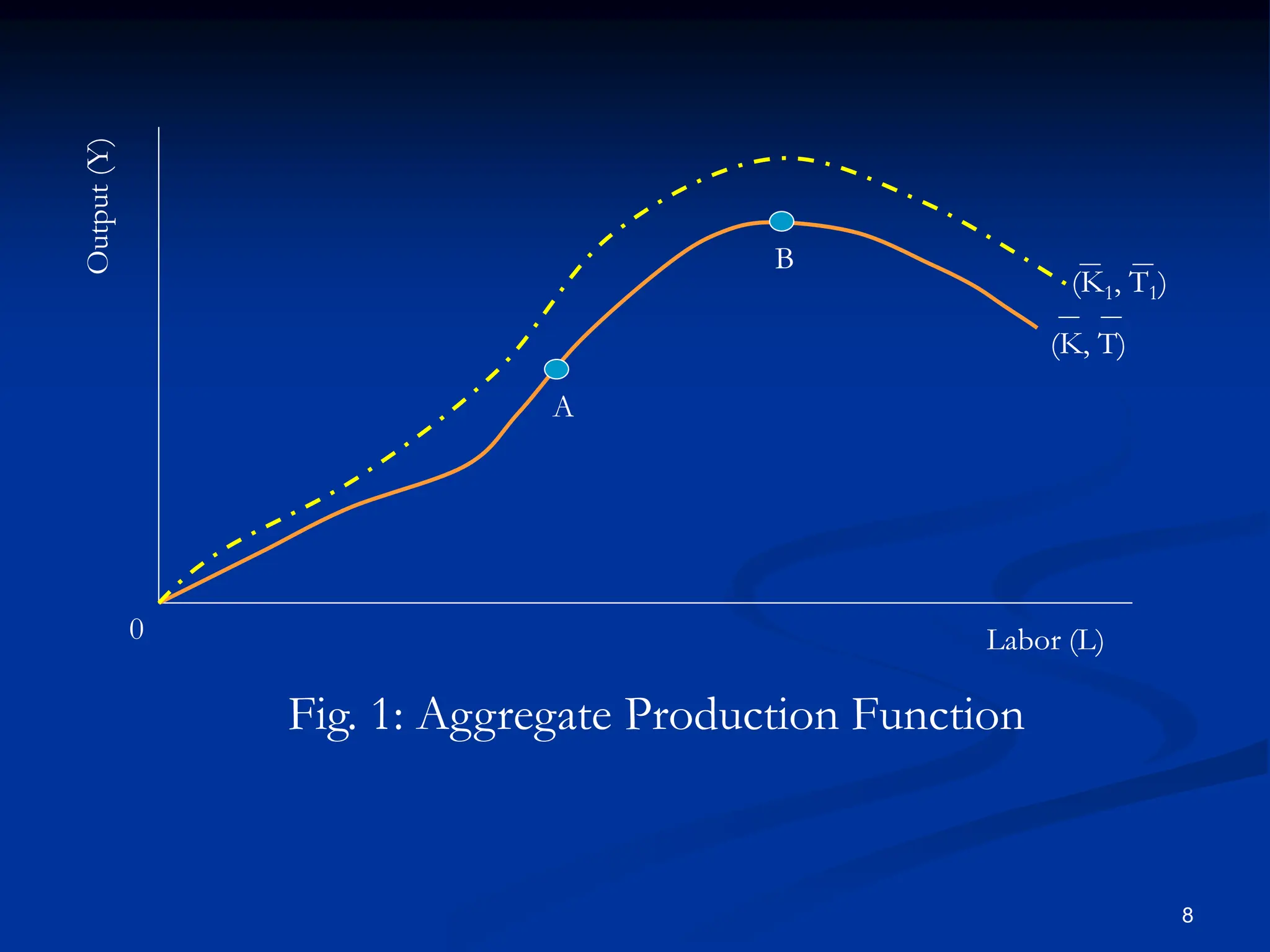
• For example, if capital increases to K1 and
technology level improves to T1, the
production function would shift upwards [see
the curve corresponding to (K1, T1)].
5.2 Demand for and Supply of Factors of
Production
• Production function is directly governed by the
factors of production, particularly labor.
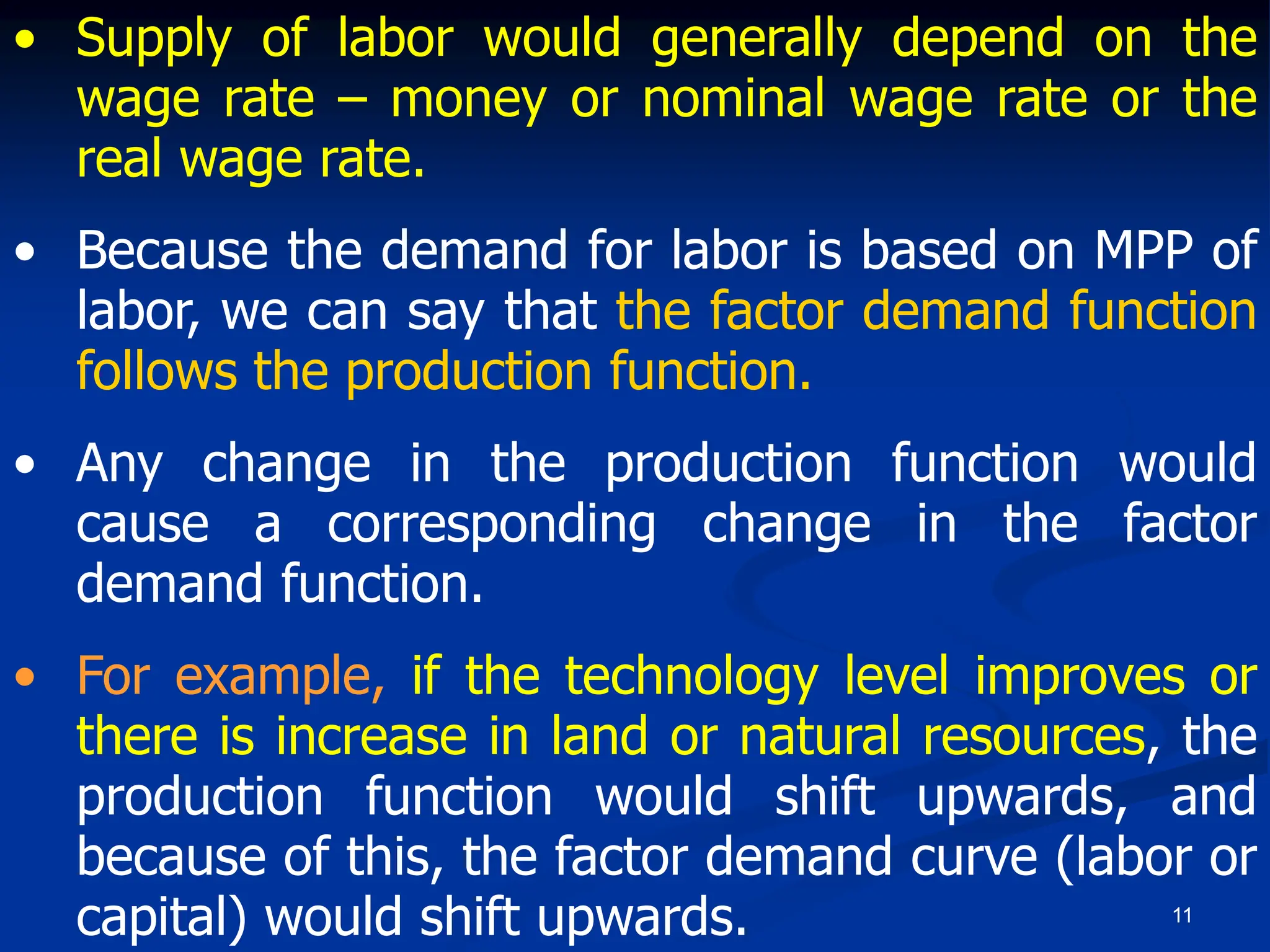
• Demand for labor would depend on the level of
output or production and the productivity
(MPP) of labor.

11. 11
• Supply of labor would generally depend on the
wage rate – money or nominal wage rate or the
real wage rate.
• Because the demand for labor is based on MPP of
labor, we can say that the factor demand function
follows the production function.
• Any change in the production function would
cause a corresponding change in the factor
demand function.
• For example, if the technology level improves or
there is increase in land or natural resources, the
production function would shift upwards, and
because of this, the factor demand curve (labor or
capital) would shift upwards.

12. 12
• For the economy as a whole, P = general price
level, W = nominal/money wage rate in the
economy, and MPP is derived from the aggregate
production function.
• The demand curve for labor is actually the MPP
curve for labor, because, given the wage rate,
different points on the MPP curve will show
demand for labor at those levels of MPP.
• A profit-maximizing firm would employ a factor up
to the point where marginal revenue productivity
(MRP) of the factor equals its marginal cost.
• For labor, MRPL = W (W is money wage rate)
MPPL = W/P (P is product price)

13. 13
DL (MPP of L)
Labor (L)
Real
Wage
Fig. 2: Demand for Labor
O

14. 14
• The slope of the demand curve for labor is
governed by the law of diminishing returns (Fig.
2).
• If there is free play of market forces, that is, if
there is wage-price flexibility, supply of labor
would vary directly with the real wage rate.
• The supply curve for labor will slope upwards
because more and more labor would be supplied
as the wage rate increases (view of the classical
economists).
• Given the demand curve for labor and the supply
curve for, labor market equilibrium under wage-
price flexibility is shown in Fig. 3.

15. 15
• Because of free play of market forces,
equilibrium is reached at L0 (L0 is equal to full
employment level Lf) and the real wage rate
(W/P)0.
• The equilibrium situation assumes perfect
competition in the labor market. This implies
that all labor units are homogeneous, inter-
occupational and spatial mobility of labor
within the economy are perfect and other
conditions of perfect competition prevail in
the labor market.

16. 16
SL
DL (MPPL)
L0 Labor
(W/P)0
Real
Wage
O
Fig. 3: Labor Market Equilibrium

17. 17
• If there is wage price rigidity, the situation would
be different with possibilities unemployment and
market disequilibrium. We find wage rigidity and
unemployment in most of the world economies
today (Keynesian economists).
• If there is wage rigidity that is, fixed money wage
rate (W0), then the real wage rate and
employment will vary according to the general
price level (P).
• For example, if the price level increases to P1 from
P0, then, given the fixed money wage rate W0,
real wage rate will decrease to W0/P and,
employment will increase to say L1 from L0
(L0≠Lf).

18. 18
• So higher the price level lower would be the real
wage rate and higher will be level of employment.
5.3 Aggregate Supply Function
• The production function and the factor market
(demand for and supply of factors of production)
together determine the aggregate supply function.
• From the factor market we know factor prices or
costs and factor supply or employment levels.
• Given a particular general price level, real wage or
labor cost in real terms (which is same as MPP)
can be known.

19. 19
• For each real wage rate and corresponding
employment level, total output that would be
produced and supplied at particular general
price level can be derived from the production
function.
• Similarly, corresponding to different general
price levels, wage rates and employment levels,
different values of aggregate output can be
determined.
• Connecting all these values, we obtain the
aggregate supply (AS) curve, because, these
values actually represent different points on the
AS curve.

20. 20
• The aggregate supply function is obtained on the
assumption that labor is the only factor of
production as we have assumed for the
production function.
• But in reality, capital, raw materials, electricity or
energy are all essential for producing output.
• When we say that the wage rate is flexible or
rigid, we also assume that prices or costs of all
other inputs are also flexible or rigid. This is done
for the sake of simplicity.
• Depending on the state of wage-price flexibility or
rigidity, three different forms of supply curve can
be obtained.

21. 21
1. AS curve under wage (nominal wage) rigidity
• It signifies perfect competition in the product
market and imperfect competition in the labor
market.
2. AS curve under price rigidity
• It reflects imperfect competition in the product
market and perfect competition in the labor
market.
3. AS curve under wage-price flexibility
• It holds on when there is perfect competition in
both product and labor markets.

22. 22
5.4 Aggregate Supply Curve: Short Run
and Long Run
• The wage rate and price level are generally
fixed in the short run but flexible in the long
run.
• The aggregate supply curves as mentioned
above in situations 1 and 2 depict two
different forms of the short-run supply curve.
• The AS curve in situation 3 shows the long-
run supply curve.

23. 23
5.4.1 AS Curve under Nominal Wage
Rigidity: Short Run
• This situation typically reflects wage settlement
or wage agreement – pattern in most of the
companies today.
• In most companies, wage settlements or
agreements between the management and the
labor unions are generally made for a period of
five years (three years in some cases) and the
nominal wage rate remains fixed during the
period of agreement.
• Under such circumstances, the labor market
becomes subject to wage rigidity.

24. 24
• The product market remains fully competitive
with flexible prices.
• Fig. 4 shown in the next slide indicate that the
AS curve is upward sloping till the point J which
corresponds to full employment level of output
(Yf) and is vertical or perfectly inelastic after
that.
• Let us assume that the nominal wage rate is
fixed at W0 and P0 is the price level at full
employment (Lf) and corresponding output level
Yf.
• If P = P0, the real wage rate is W0/P0. At this
real wage rate, demand for labor is Lf which
corresponds to output Yf.

25. 25
G
H
J
K
AS
P
P1
P0
P2
P3
Y3 Y2 Yf Y
O
Fig. 4: Short Run AS Curve under Nominal Wage Rigidity

26. 26
• Now, let us assume that the price level increases to
P1 (P1>P0) because of increase in aggregate
demand.
• Because P = P1, the real wage rate decreases to
W0/P1.
• At this lower wage rate, demand for labor increases
to , say, L1 (L1>Lf).
• But, because, full employment level has already
been reached, there is no supply of labor beyond Lf.
• Therefore, although the real wage rate is lower,
supply of labor still remains restricted to Lf because
no excess labor is available for employment and
output remains constant at Yf level.

27. 27
• Therefore, for any P>P0, the AS curve will be
vertical or perfectly inelastic at Yf level.
• Let us now assume that the price level falls to P2
(P2<P0). This can happen if aggregate demand
falls.
• If price falls from P0 to P2, the real wage rate
increases to W0/P2.
• At this real wage rate, demand for labor
decreases to , say, L2 (L2<Lf).
• Corresponding to labor employment of L2 output
would fall to Y2 (known from the production
function).

28. 28
• If the price level falls further to P3, the real
wage rate will increase further to W0/P3,
demand for labor will fall further and output
will fall to Y3. This is shown by point G on the
AS curve.
• The assumption of wage rigidity in the short
run may appear quite reasonable.
Wage/salary contracts are very common in
most of the business organizations and
wages/salaries change only once in two or
three years.

29. 29
5.4.2 AS Curve under Price Rigidity:
Short Run
• If there is imperfect competition in the
product market, prices will not move freely.
In fact, the price level may remain rigid
during a particular period (short run). This
will happen particularly if there is
dominance of monopoly firms. The labor
market, however, still remains perfectly
competitive with flexible wages.

30. 30
• Because of price rigidity, but flexible wage
rate, the AS curve is horizontal or perfectly
elastic up to a point, and after that becomes
vertical or perfectly inelastic.
• In Fig. 5, the AS curve is perfectly elastic up to
point J, and perfectly inelastic after that with
corresponding price, wage, employment and
output levels.
• Let P0 be the fixed price level. If aggregate
demand increases (from the existing level),
firms can increase output to meet the
additional demand.

31. 31
AS
K
J
P
P1
P0
P2
O Yf Y
Fig. 5: Short run AS Curve under Price Rigidity

32. 32
• They can do this by employing more labor by
paying higher nominal, and also real, wage till
the full employment level (Lf) is reached.
• Firms can pay higher nominal wage because
the wage rate is flexible and, also higher real
wage rate because price is fixed and,
therefore, higher nominal wage would also
mean higher real wage.
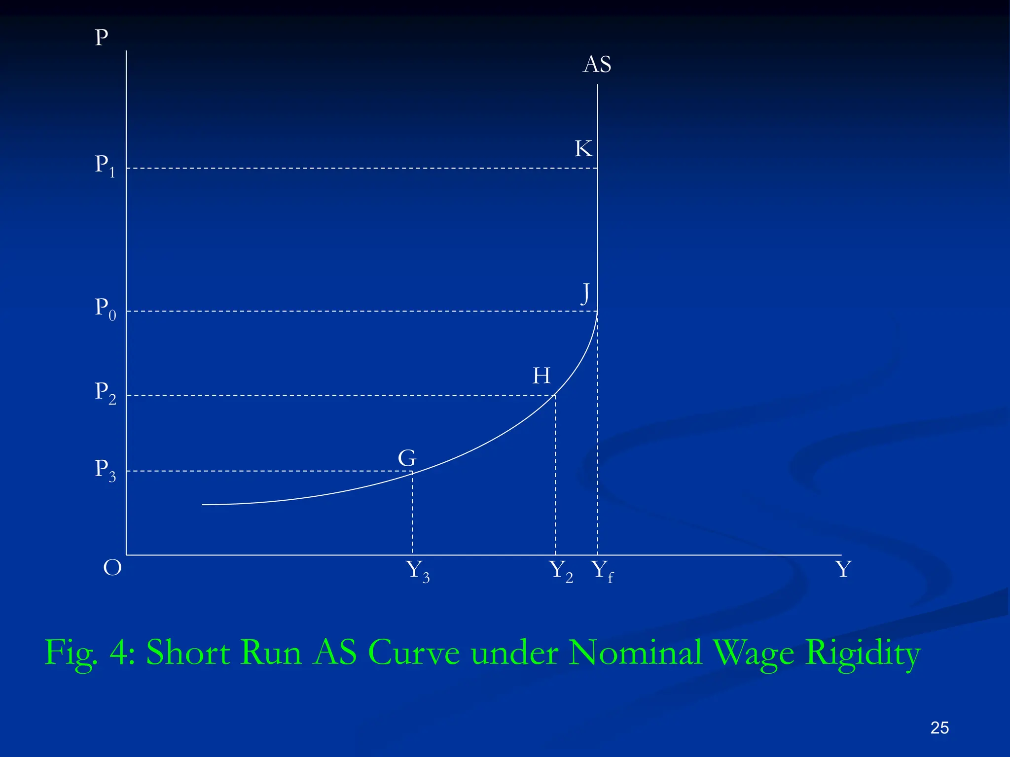
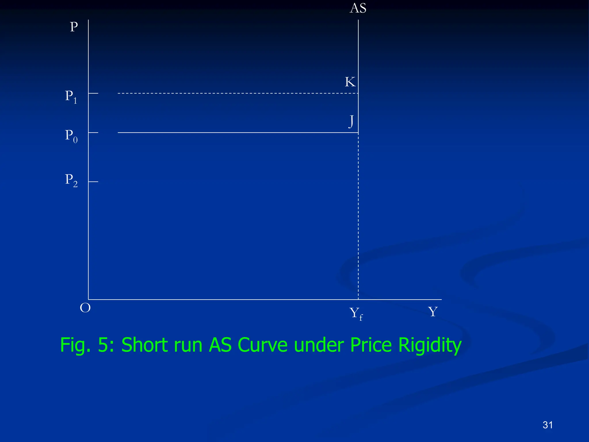
• So, at fixed price level P0, output will increase
till the full employment level of output Yf is
reached [shown by the perfectly elastic part
(P0J) of the AS curve].

33. 33
• After the full employment level of output is
reached, there will be no further increase in
production and supply even if aggregate
demand increases, because, no more labor
is available for employment [shown by the
perfectly inelastic part (JK) of the AS
curve].
• But, the assumption of price rigidity or
fixed price seems to be unreasonable even
in the short run.

34. 34
• If there is an increase in the costs of variable
inputs like raw materials, fuel or electricity, firms
may be under compulsions to increase prices of
their products; otherwise, their margins may be
reduced or eroded.
• Also, inflation (cost push or demand pull) is a
common characteristic of most of the economies
today.
5.4.3 AS Curve under Wage-Price Flexibility:
Long Run
• In the long run, both the price level and the
wage rate are flexible and move according to
market condition.

35. 35
• With no imperfections in the labor market, the
money wage rate would be flexible
downwards.
• At any time, if supply of labor exceeds
demand for labor, competition for jobs among
workers would result in a fall in the money
wage rate and vice versa.
• With the price level also flexible, the AS curve
in the long run would be perfectly inelastic.
• Fig. 6 shows that, in the long run, aggregate
supply or output is independent of the price
level.

36. 36
• Supply remains constant at full employment
output Yf. Because of flexibility in the labor
market, full employment (Lf) will be always
ensured through adjustment in the nominal
wage rate (the classical theory of full
employment equilibrium).
• If the price level is P0 and the corresponding
money wage rate is W0, full employment real
wage rate is (W/P)0 = (W/P)f. This is shown by
point J.
• If the price level increases to P1, because of
increase of aggregate demand, output should
increase to meet the additional demand, and,
demand for labor should increase.

37. 37
O Yf Y
H
J
K
AS
P
P1
P0
P2
Fig.6: Long Run AS with Wage-Price Flexibility

38. 38
• But, because output is constant at Yf level,
excess demand for labor would lead to an
increase in the nominal wage rate to W1, which
is proportional to P1, so that, real wage rate is
maintained at the full employment level (W/P)1
= (W/P)f.
• If price falls to P2, excess supply of labor will
push down the nominal wage rate to W2 so that
(W/P)2 = (W/P)f and full employment is
maintained.
• This shows that equilibrium in the labor market
is consistent with different price levels, but only
one level of output, that is, Yf.

39. 39
• Any change in the price and, in aggregate
demand would cause a proportional or equal
change in the money wage rate so that
constancy of the real wage rate and full
employment level is maintained.
• Figures 4, 5 and 6 show that differences in the
shapes of AS curve under nominal wage rigidity
(short run), price rigidity (short run) and, wage-
price flexibility (long run) exist till full
employment output is reached.
• At the full employment output level, all the three
AS curves are perfectly inelastic.

40. 40
• Because of wage and price rigidity in the short-
run, full employment equilibrium may not be
reached, and, output may remain below the full
employment level. Once the full employment
level of output (Yf) is reached, there will be no
further increase in output because of
diminishing marginal productivity of labor.
• Output will not increase further even if there is
constant marginal productivity of labor.
• With full employment labor supply, output can
increase beyond Yf only if there is increase in
labor productivity, that is, if there is increasing
marginal productivity of labor, but, this is very
unlikely.

41. 41
• Aggregate supply or output can increase if
there is a rightward shift in the AS curve. This
can happen because of change in a number of
factors which have so far been assumed to
remain constant.
• Three major factors, which can cause a
rightward shift in the AS curve are increase in
the labor force, increase of capital and
improvement in the level of technology (all
these changes are likely to take place in the
long run and not in the short run).

42. 42
5.5 Aggregate Demand and Aggregate
Supply
• Because of rise or fall in the general price level,
aggregate demand decreases or increases.
• The process of change in demand for real
output (at constant prices) takes place through
the monetary system, or, more precisely,
through demand for and supply of money – real
money or real cash balances – and, the interest
rate.
• Real money supply is defined as money supply
(M3) divided by the price level (P)

43. 43
• Let us assume that the price level falls. Given a
particular level of money supply, if price falls, real
money or real cash balances increase. This means
that the public is now holding larger real money
balances than it wishes to hold.
• The excess real money balances will be
used/diverted to purchase of bonds by the people.
• This will push up the bond prices and lower the
interest rate. As the interest rate falls, investment
increases.
• This means that, other things being equal, total
amount of goods demanded (to meet the new
investment demand), i.e., aggregate demand
increases.

44. 44
• Similarly, the opposite happens when the price
level increases.
• Because of the inverse relationship between the
price level and aggregate demand, the AD curve
will be downward sloping.
• The general shape of the AD curve is same as
that of the demand curve facing an individual
firm.
• The AS curve may have more than one form
and shape depending on whether we make the
Keynesian assumption of wage/price rigidity or
the classicists’ assumption of wage – price
flexibility (already discussed).

45. 45
Y
Yf
Y2
Y0
Y1
O
P2
P0
P1
A
AD
AS
P
Fig. 7: Equilibrium Price and Output:: Keynesian Model

46. 46
• Equilibrium levels of price and output with
wage rigidity is shown in Fig. 7. The figure
shows that equilibrium is at point A and
equilibrium levels of price and output are P0
and Y0.
• It is found from the figure that equilibrium
output Y0 is less than the full employment
level Yf.
• The shape of the AS curve shows that, if there
is a significant rightward shift in the AD curve,
both price and output will increase, and, there
is possibility of full employment equilibrium.

47. 47
• In fact, although the Keynesian approach
stipulates that equilibrium below full
employment is a realistic possibility, it does not
completely rule out full employment
equilibrium.
• The classical approach states that full
employment equilibrium is the only possibility
(Fig. 8).
• The AS curve is vertical or perfectly inelastic at
full employment level of output (Yf). AD
intersects AS at point A which gives the
equilibrium price as P0.

48. 48
Y
Yf
O
A
AS
AD1
AD0
AD2
P
P0
P1
P2
Fig. 8: Equilibrium Price and Output: Classical Model

49. 49
• The relevance of the classical model of almost
automatic full employment equilibrium is being
questioned today.
• With high rates of unemployment in countries
like Cambodia and many other countries, less
than full employment equilibrium output,
wage/price rigidity and market imperfections
seem to more realistically characterize most of
the modern economic system.